Multi-Agent Coverage Path Planning Using Graph-Adapted K-Means in Road Network Digital Twin

Abstract

In this paper, we research multi-robot coverage path planning (MCPP), which generates paths for agents to visit all target areas or points. This problem is common in various fields, such as agriculture, rescue, 3D scanning, and data collection. Algorithms to solve MCPP are generally categorized into online and offline methods. Online methods work in an unknown area, while offline methods generate a path for the known. Recently, offline MCPP has been researched through various approaches, such as graph clustering, DARP, genetic algorithms, and deep learning models. However, many previous algorithms can only be applied on grid-like environments. Therefore, this study introduces an offline MCPP algorithm that applies graph-adapted K-means and spanning tree coverage for robust operation in non-grid-structure maps such as road networks. To achieve this, we modify a cost function based on the travel distance by adjusting the referenced clustering algorithm. Moreover, we apply bipartite graph matching to reflect the initial positions of agents. We also introduce a cluster-level graph to alleviate local minima during clustering updates. We compare the proposed algorithm with existing methods in a grid environment to validate its stability, and evaluation on a road network digital twin validates its robustness across most environments.

1. Introduction

Digital twin and immersive environments are increasingly used to synchronize and mirror physical spaces in real time [1]. To maintain such synchronization, continuous sensing of the real-world environment is required [2]. One effective approach is to employ multiple agents that can collectively perform tasks across a wide area [3,4,5,6]. In order for these agents to efficiently and periodically cover the environment, multi-agent coverage path planning (MCPP) is essential.

MCPP involves generating paths for agents to visit all given points of interest or areas. The path is generated to efficiently traverse the points of interest while avoiding collisions with obstacles and other agents. This problem has broad applications across various domains, such as disaster areas [7], data collection [8,9], monitoring [10,11], agriculture [12], 3D scanning [13], and autonomous robots [14].

MCPP is primarily divided into online and offline methods based on the prior knowledge and situation of the target environment. Online MCPP generates paths for either unknown or dynamic areas. For instance, when agents investigate an unexplored area, path modification is necessary to avoid unexpected obstacles or explore unvisited regions [15]. Meanwhile, during the task, when the number of agents changes, path redesign becomes essential [16].

Due to these conditions, the algorithm must operate in real time. Therefore, online MCPP has been studied through reinforcement learning [17], artificial potential fields (APFs) [18], etc. Moreover, integrating these approaches with immersive VR/AR interfaces can support human-in-the-loop monitoring and the intuitive visualization of agent coverage and coordination.

Conversely, offline MCPP generates a complete coverage path for a known environment. Unlike online methods, it does not require real-time path modification. Moreover, due to prior knowledge of the environment, this method tends to generate a more optimized path than the former approach. It is mainly researched using divide and conquer methods such as graph partitioning [19], clustering [20], spanning tree coverage (STC) [21], and genetic algorithms [22].

Previous studies on graph-based methods typically employ grid graphs, where the target area is divided into uniform cells. This structure features uniform vertex degrees and a regular arrangement of edges. However, these characteristics are not always guaranteed. Consider a scenario where agents are traversing a non-grid road network digital twin, as in Figure 1. To address this, the environment should be represented as a non-grid graph with weighted edges. Therefore, we present a clustering-based offline MCPP method applicable to non-grid graphs. The contributions of this paper are as follows.

1.

We implement an objective function based on STC by modifying the weights of graph-adapted K-means [23].

2.

We apply an optimized merging method on the update step based on [23] to prevent the graph separation problem.

3.

We develop a cluster propagation method using a cluster-level graph to alleviate the local minima problem.

2. Related Works

With advances in computational power and communication technologies, multi-agent systems have been drawing significant attention. These systems enable the manipulation of agents in a digital twin to perform collaborative tasks in the real world. For instance, there are cases where multiple virtual agents are employed to efficiently generate paths for each agent in order to conduct large-scale 3D scanning. For example, ref. [3] extracts a skeleton of the central traversable paths in the map and divides it into multiple agent paths while considering physical constraints. Meanwhile, ref. [5] generates paths for unmanned aerial vehicles (UAVs) to scan occluded parts of a structure by scheduling exploration plans on a coarse-terrain digital twin via solving the traveling salesman problem. Similarly, there are also studies on swarm robot control within digital twin environments. For example, ref. [1] demonstrates a control approach where humans issue commands only to a small set of virtual agents in the VR. Each agent controls subordinate robot groups via its hierarchical digital twin, while path coordination ensures collision avoidance. These approaches commonly reinterpret continuous digital twin spaces into alternative forms and generate paths via vertex traversal problems.

MCPP can be classified into centralized and decentralized approaches based on how agents coordinate [20]. In a centralized approach, a single solver with global information generates paths and controls the agents. Conversely, in decentralized methods, each agent has local information and constructs its own paths through cooperation with other agents. Consequently, the centralized method typically requires substantial computational resources but yields more efficient paths. For these reasons, offline methods are typically employed, coupled with centralized approaches. Previous studies have implemented this method by partitioning the environment into discrete units and then generating paths.

Graph-based approaches rasterize the environment [10,24] into a grid map or an adjacency graph through cellular decomposition [25,26]. Then, independent subgraphs are formed via clustering, and a path is generated for each cluster. In this process, cellular decomposition employs path patterns such as back and forth or zigzag [26]. When using a grid map, graph traversal methods such as Euler circuits [27] and spanning tree coverage (STC) [21] are commonly adopted for coverage tasks.

Ref. [10] converts the entire area into a grid of square cells and then applies K-means using the centers of the Voronoi diagram as cluster centroids. Because the boundaries of this diagram are similar to the criteria for cluster partitioning, cells that include a boundary become ‘conflict points’ that are not clearly assigned to any cluster. In this study, these cells are allocated to neighboring clusters with lower weights, creating clusters in which the workload is equally distributed. Nikolaos [18] employed affinity propagation clustering. After forming initial clusters, the method calculates the similarity based on a four-grid distance to revise the clusters so that travel distances are evenly balanced.

STC [21] first constructs a minimum spanning tree (MST) of the given graph and then generates a path that circumnavigates it. Expanding on this, multi-robot STC (MSTC) [24,28], for multiple agents, creates a traversal path in the same manner and allocates segments of the tree between adjacent agents. However, if agents are positioned too closely, they all move in the same direction, causing the allocation to fail. Although the same study proposed a backtracking approach that revisits previously covered paths to mitigate this issue, optimal allocation was still not achieved.

To address this problem, multi-robot forest coverage (MFC) divides the entire tree into several balanced subgraphs [29]. Later, MSTC* [30] was introduced to incorporate physical constraints—such as terrain traversability and material load capacity—into a cost-based framework. Similar to MFC, this method partitions the entire tree equally and propagates coverage among neighboring agents. More recently, researchers have explored minimum-turn MSTC* (TMSTC*) [31], which uses linear block segments based on tree branches to reduce the number of agent rotations, as well as an online method that adapts to real-time weight changes [32].

Divide Area based on Robot’s Initial Positions (DARP) [33] performs area partitioning by optimizing a cost function defined using the distance matrix between robots’ initial positions and all vertices. This cost function is designed based on two criteria, namely cluster connectivity and workload balance, and is computed according to the distances from the initial positions to the vertices. The optimization proceeds by iteratively reassigning vertices adjacent to clusters, which allows DARP to achieve optimal solutions compared to other algorithms. However, it suffers from a high computational cost and may lead to imbalanced partitions in cases where bottlenecks occur around the initial positions.

Reinforcement learning can be deployed to solve this problem. For example, [34] addresses decentralized multi-robot coverage path planning by framing subarea allocation as a sequential decision-making task with reinforcement learning. Robots expand their territories using local observations enriched with structural and neighbor information. A neural network policy directs these expansions, while robots may pause expansion to prevent unnecessary overlaps. The method yields balanced subareas with minimal overlap and scales to larger maps and more agents, although training is difficult due to delayed rewards and can be unstable, occasionally producing imbalanced partitions.

Ref. [35] performs cooperative coverage path planning by first partitioning the environment with an improved K-means clustering algorithm that incorporates MST to achieve more balanced divisions. After partitioning, each robot is assigned to a subarea and applies deep reinforcement learning with a dueling network structure. An improved reward function guides robots away from redundant paths and toward unexplored regions, enabling more efficient coverage. This framework achieves higher coverage ratios and reduced path duplication relative to single-robot methods. However, these approaches remain sensitive to the reward design, which can lead to imbalanced paths.

3. Problem Statement

The target environment graph is defined as $\mathrm{G}=(\mathrm{V},\mathrm{E},\mathrm{W})$, where $\mathrm{V}=\{v_1\dots v_n\}$ is the set of vertices and $\mathrm{E}=\{e_1\dots e_m\}$ is the set of edges. $\mathrm{W}=\{w_1\dots w_m\}$ is the set of edge weights, and $w_x$ represents the weight assigned to edge $e_x$. The number of agents is represented by k. The initial positions of each agent are defined as $\mathrm{S}=\{s_1\dots s_k|s\in \mathrm{V}\}$. The path generation algorithm F is a function that outputs a set of paths by taking a graph and an initial position, as shown in Equation (1). $\mathrm{P}=\{p_1\dots p_k\}$ represents the collision-free paths assigned to each agent. Meanwhile, $p_i$ is a set of path vertices with length l, $p_i=\{v_{i1}\dots v_{il}\}$.

$$\mathrm{F}(\mathrm{G},\mathrm{S})=\mathrm{P}$$

(1)

Path group $\mathrm{P}$ must visit every vertex of the graph at least once. Furthermore, consider that each path must have the optimal traversal time. Therefore, we set the goal as the ideal path group ${\mathrm{P}}^{*}$ in Equation (2), where $T\left(p_i\right)$ indicates the total traversal time of $p_i$.

$${\mathrm{P}}^{*}={argmin}_{\mathrm{P}}\max \left(T\left(\mathrm{P}\right)\right),(\mathrm{V}\in \bigcup _{\mathrm{P}}{p}_i)$$

(2)

4. Proposed Methods

4.1. Graph Adapted K-Means

Graph-adapted K-means [23], proposed by Sieranoja and Fränti, is a clustering method that considers the edge weights of the graph. This algorithm utilizes three types of costs with iterative clustering and merging. Specifically, we focus on the inverse internal weight (IIW) cost.

To explain the IIW, a graph $\mathrm{G}=(\mathrm{V},\mathrm{E})$ is defined. The weight of the edge between vertices i and j is defined as $w_{ij}$. At this time, if a cluster $\mathrm{X}$ consists of $n_x$ vertices, the sum of the weights of the internal edges is defined as $W_x$. The sum of the weights of the edges connected to the other cluster is expressed as $E_x$. For example, calculating the values according to the above definition for the graph in which all edge weights are one, as shown in Figure 2, gives the metrics listed in

Table 1. Variables of the example graph.

Cluster	${\mathit{n}}_{\mathit{x}}$	${\mathit{W}}_{\mathit{x}}$	${\mathit{E}}_{\mathit{x}}$
A	4	8	2
B	3	6	2

.

IIW is the average of the reciprocals of the sums of $W_x$ in each cluster, as shown in Equation (3), where M is the sum of the weights of all edges in the graph. This cost is scaled to the range $[1,\infty ]$, with smaller values meaning better clustering. As a result, it aims to assign the same weight to all clusters. In the case of optimal clustering, all clusters have a ’mean weight of a perfectly balanced cluster’ ($M/k$).

$$\mathrm{IIW}={\displaystyle \frac{M}{k}}{\displaystyle \frac{1}{k}}\sum _{i=1}^k{\displaystyle \frac{1}{W_i}}$$

(3)

As mentioned above [23], the method consists of two algorithms: the K-algorithm (clustering) and the M-algorithm (merging). The K-algorithm tracks the cost by delta calculation, as shown in (4), when assigning a vertex j in cluster $\mathrm{X}$ to a neighbor cluster $\mathrm{Y}$. $C_{\mathrm{X}}$ and $C_{\mathrm{Y}}$ are the subgraphs of each cluster before the change, while $C_{\mathrm{X}}^{\prime }$ and $C_{\mathrm{Y}}^{\prime }$ are those after the change. Then, the vertex is assigned to the cluster with the optimal $\Delta f(j,\mathrm{X},\mathrm{Y})$. This approach reduces the computational cost by avoiding the calculation of the average value of the cluster in each iteration.

$$\begin{array}{c}\hfill \Delta f(j,\mathrm{X},\mathrm{Y})=\Delta f\left(C_{\mathrm{X}}\right)+\Delta f\left(C_{\mathrm{Y}}\right)=f\left(C_{\mathrm{X}}^{\prime }\right)+f\left(C_{\mathrm{Y}}^{\prime }\right)-f\left(C_{\mathrm{X}}\right)-f\left(C_{\mathrm{Y}}\right)\end{array}$$

(4)

The M-algorithm operates by repeating these operations until the cost converges or the maximum number of iterations is reached.

1.

Select and merge two randomly selected adjacent clusters.

2.

Split one random cluster into two.

3.

Apply the K-algorithm.

However, the split–merge process can cause substantial shifts in cluster centroids, which increases the errors in path generation. Therefore, the proposed algorithm incorporates the K-algorithm and the merging method in the M-algorithm.

4.2. Distance-Based Cost Function

To enable the use of STC in non-grid environments, we design the cost function as follows. While the conventional spiral STC operates only on grid graphs [21], it is possible to construct a coverage path based on MST [30]. This enables the derivation of a traversal path in weighted non-grid graphs using algorithms such as depth-first search. In the ideal case, each agent would be assigned an equally partitioned subtree. However, when the initial positions of agents are distant from their assigned cluster, additional travel costs are incurred, which may result in an imbalance in workload distribution. To address this, we divide each agent’s route into an initial travel path and a coverage path and define the target cluster size of each agent in proportion to the length of these paths. Finally, the cost is computed as the error between the ratio of the desired cluster sizes and the ratio of the actual path lengths.

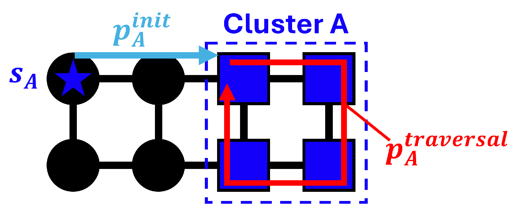
In this paper, we assume that the movement speed of all agents is the same, denoted as v. For this reason, the travel distance of path $D\left(p_i\right)$ is expressed as $D\left(p_i\right)=T\left(p_i\right)\ast v$, and Equation (2) can be written as Equation (5). This implies that all paths in $P^{*}$ will have the same travel distance. To calculate the distance, we separate $p_i$ into the initial path $p_t^{init}$ and the traversal path $p_t^{traversal}$. As shown in Figure 3, $p_i^{init}$ denotes the path from an initial position to the cluster, whereas $p_i^{traversal}$ refers to the Euler circuit within it. Thus, $D\left(p_i\right)$ equals the sum of the distances of the two parts, which matches Equation (6).

$${\mathrm{P}}^{*}={argmin}_{\mathrm{P}}\max \left(D\left(\mathrm{P}\right)\right),(\mathrm{V}\in \bigcup _{p_i}{p}_i)$$

(5)

$$D\left(p_i\right)=D\left(p_i^{init}\right)+D\left(p_i^{traversal}\right)$$

(6)

Considering Equation (6), to satisfy ${\mathrm{P}}^{*}$, the relative distances of the two parts between clusters must be taken into account, i.e., if $D\left(p_i^{init}\right)$ is relatively high, then $D\left(p_i^{traversal}\right)$ should be low. Additionally, we utilize IIW for the cost function, which is ideal when all clusters have the same sum of internal weights $(M/k)$. According to this, we calculate the target ratio of the traversal distance ${\mathrm{R}}_i$ as in Equation (7), where $d^{*}$ is the optimally distributed traversal distance. We define this as the traversal length of a global minimum spanning tree equally divided into k segments, as in Equation (8). Then, we calculate ${\mathrm{R}}_i$ as

$${\mathrm{R}}_i={\displaystyle \frac{{\sum }_{z=1}^{k}D\left(p_z^{init}\right)-D\left(p_i^{init}\right)+d^{*}}{{\sum }_{j=1}^k({\sum }_{z=1}^{k}D\left(p_z^{init}\right)-D\left(p_j^{init}\right)+d^{*})}},\sum _{i=1}^k{\mathrm{R}}_i=1$$

(7)

$$d^{*}={\displaystyle \frac{2{\sum }_{MST\left(\mathrm{G}\right)}{w}_i}{k}}$$

(8)

Finally, we define the cost function $C\left(\mathrm{P}\right)$ as the absolute sum of the errors between the actual ratio of $D\left(p_i^{traversal}\right)$ and ${\mathrm{R}}_i$, as in Equation (9). This cost ranges within $[0,k)$, and a lower value indicates better clustering. Accordingly, the target path set ${\mathrm{P}}^{*}$, denoted as in Equation (5), can be expressed as in Equation (10).

$$C\left(\mathrm{P}\right)=\sum _{i=1}^k\left|{\displaystyle \frac{D\left(p_i^{traversal}\right)}{{\sum }_{z=1}^{k}D\left(p_z^{traversal}\right)}}-{\mathrm{R}}_i\right|$$

(9)

$${\mathrm{P}}^{*}=argmi{n}_{\mathrm{P}}C\left(\mathrm{P}\right),(\mathrm{V}\in \bigcup _{p_i}{p}_i)$$

(10)

4.3. Initialization Step

In the initialization step, the initial clusters and ${\mathrm{R}}_i$ are computed based on the agent’s position. The pipeline is described in Algorithm 1. First, we apply region-growing base initialization [23]. The extension of cluster i starts at $s_i$, targeting its neighboring vertices, and continues until the cluster contains at least $\left|\mathrm{V}\right|/k\ast 0.8$ [23] of vertices or when the internal weight reaches $d^{*}$. However, it blocks other $s_i$, making it impossible to expand. In this case, we change the blocked position to a new vertex that has the highest density as calculated via $density\left(v_x\right)={\sum }_{j\in neighbor\left(v_x\right)}{w}_{xj}$. Despite efforts to avoid blocking, some vertices may remain unassigned. Consequently, they are assigned to the adjacent cluster with the highest edge weight.

Algorithm 1 Initialization Step

1: Input: $\mathrm{G}$, $\mathrm{S}$ 2: Output: cluster, $\mathrm{R}$, ${\mathcal{M}}_{\mathrm{B}}$ 3:    cluster = initialize cluster 4:    cluster = assign remaining vertices 5:    $\mathrm{B}$ = construct bipartite graph 6:    ${\mathcal{M}}_{\mathrm{B}}$ = perfect minimum matching on $\mathrm{B}$ 7:    $\mathrm{R}$ = cal target ratio by ${\mathcal{M}}_{\mathrm{B}}$

As we update $s_i$, there is a $D\left(p_i^{init}\right)$ because the agent was not contained in the cluster. To obtain an optimized ${\mathrm{R}}_i$, we perform perfect minimum bipartite matching. Therefore, we define a complete bipartite graph as $\mathrm{B}=({\mathrm{V}}_{agent},{\mathrm{V}}_{cluster},{\mathrm{E}}^{\prime },{\mathrm{W}}^{\prime })$, where $|{\mathrm{V}}_{agent}|=|{\mathrm{V}}_{cluster}|=k$. An edge $e_{ij}^{\prime }$ in ${\mathrm{E}}^{\prime }$ denotes the path from $s_i$ to cluster j. The weight of this edge, which is an element of ${\mathrm{W}}^{\prime }$, corresponds to the distance of its path. A visualization of $\mathrm{B}$ is provided in Figure 4. As a result, we compute the bipartite matching ${\mathcal{M}}_{\mathrm{B}}$, followed by the calculation of $\mathrm{R}$.

4.4. Update Step

In the update step, clusters are iteratively refined according to cost $C\left(\mathrm{P}\right)$. This step consists of a K-step and M-step, as mentioned in Section 4.1. The algorithm follows the process outlined in Algorithm 2. The K-step applies to all vertices that are on the cluster’s boundary. If a decrease in cost is observed, the update is accepted. To incorporate delta calculation into this process, we reformulate the cost function as in Equation (11), where ’−’ indicates the cluster from which a vertex is removed and ’+’ denotes the one to which it is added. Moreover, $\Delta W_x$ represents the change in cluster weight, while $W_x^{prev}$ indicates the prior value.

$$C\left(\mathrm{P}\right)=\sum _{i=1}^k\left|{\displaystyle \frac{2W_i^{prev}+\Delta W_i}{{\sum }_{z=1}^{k}2W_z^{prev}+\Delta W_{+}+\Delta W_{-}}}-R_i\right|$$

(11)

Algorithm 2 Update Step

1: Input: $\mathrm{G}$, cluster, $\mathrm{R}$, MAX_ITER, THRESHOLD 2: Output: cluster 3: for iter = 0 : MAX_ITER do 4:    update by K-step 5:    merge isolated component by M-step 6:    if C(P) < THRESHOLD then 7:      break 8:    end if 9: end for

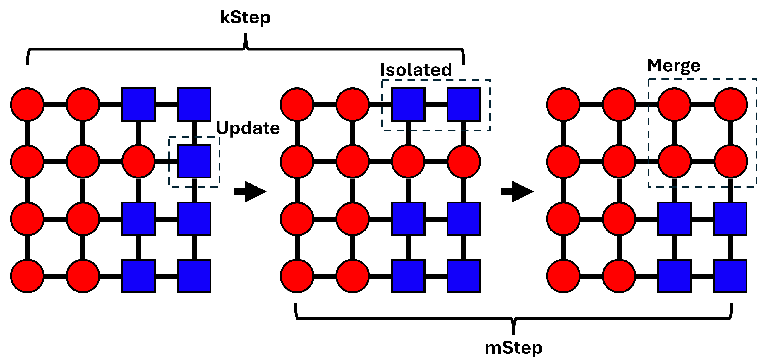
However, in the K-step, a single cluster may fragment into multiple connected components. For example, as seen in Figure 5, if a vertex in the blue cluster is updated to the red cluster, the former inevitably splits into two disconnected components, making pathfinding more difficult. In the M-step, these fragments are merged into another cluster. We define a cluster’s connected components as ’isolated’, except for the largest one. These isolates are merged into adjacent clusters. If multiple neighboring ones exist, the one with the lowest $W_i$ after merging is selected. This process is applied to all isolated components. The two steps are repeated until the cost converges below a certain threshold (THRESHOLD) or the maximum number of iterations (MAX_ITER) is reached.

4.5. Path Generation

After clustering, traversal paths are generated using STC. Since clusters do not share vertices, collisions between agents over $p^{traversal}$ do not occur. However, $p^{init}$ may overlap with other clusters, potentially causing collisions. To mitigate this, we adapt Windowed Hierarchical Cooperative A* (WHCA*) [36] for initial path generation. The modified algorithm finds the nearest vertex $t_i$ within an agent’s assigned cluster from $s_i$. Then, we calculate the A* path between two vertices. After the agent reaches $t_i$, its $p^{traversal}$ is incorporated into the window to ensure a collision-free path.

5. Cluster Propagation Using Cluster-Level Graph

5.1. Local Minima Problem

The K-step in Section 4.4 considers only neighboring clusters when updating a vertex. This is not an issue in a simple environment, i.e., with fewer agents and a simple graph structure. In contrast, the local minima problem may arise due to failed cluster propagation. For instance, consider two situations where $\mathrm{G}$ is a $3\times 3$ 4-grid graph with $k=2$ (a) and $k=4$ (b), as shown in Figure 6. At this point, assume that transferring a vertex from cluster 2 to cluster 1 is required to achieve the optimal $\mathrm{R}$. Additionally, clusters 3 and 4 in (b) are defined as having the optimal weight. In case (a), the update will succeed since the two clusters are adjacent. On the other hand, in scenario (b), clusters 3 and 4 lie between them, preventing direct vertex transfer. However, as the K-step rejects updates that increase the cost, propagation may fail, potentially leading to the local minima problem. To address this issue, we designate the global source and destination clusters from the cluster-level graph in each update.

5.2. Update Step Using Cluster-Level Graph

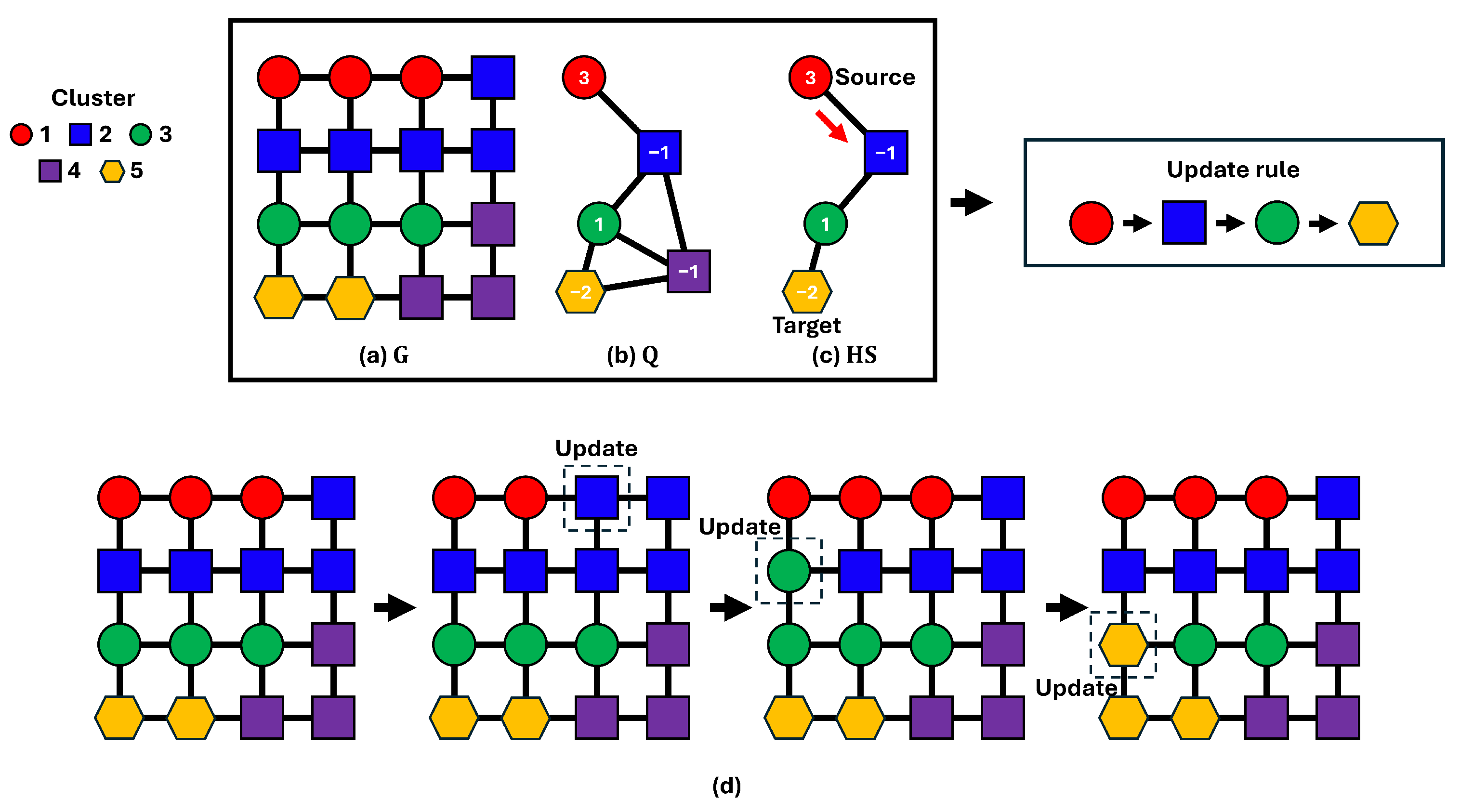
We define a cluster-level graph as $\mathrm{Q}=\{{\mathrm{V}}^{\mathrm{Q}},{\mathrm{E}}^{\mathrm{Q}},{\mathrm{VW}}^{\mathrm{Q}}\}$, where vertices ${\mathrm{V}}^{\mathrm{Q}}=\left\{v_i^{\mathrm{Q}}\right\}$ indicate cluster i. The edge $e_{ij}^{\mathrm{Q}}$ is formed when the two clusters i and j are neighbors. The vertex weight $v{w}_i^{\mathrm{Q}}$ is calculated as in (12), which represents the deviation of $\mathrm{R}$ for the cluster. A negative value indicates insufficient weight, a positive value indicates excess, and, lastly, an optimally balanced cluster has a value of zero. An example of $\mathrm{Q}$ is illustrated in Figure 7b.

Figure 7. The K-step process with cluster-level graph $\mathrm{Q}$. Each color of the vertices represents a distinct cluster. (a) Target environment graph $\mathrm{G}$; (b) cluster-level graph $\mathrm{Q}$, where the numbers on each vertex indicates the vertex weight $v{w}_i^{\mathrm{Q}}$; (c) the shortest path $\mathrm{HS}$ between the global source ($v_{\max }^{\mathrm{Q}}$) and destination ($v_{\min }^{\mathrm{Q}}$); (d) the K-step process follows the update rule derived from $\mathrm{HS}$. Despite applying this process, isolated components may still emerge, requiring correction in the M-step.

Figure 7. The K-step process with cluster-level graph $\mathrm{Q}$. Each color of the vertices represents a distinct cluster. (a) Target environment graph $\mathrm{G}$; (b) cluster-level graph $\mathrm{Q}$, where the numbers on each vertex indicates the vertex weight $v{w}_i^{\mathrm{Q}}$; (c) the shortest path $\mathrm{HS}$ between the global source ($v_{\max }^{\mathrm{Q}}$) and destination ($v_{\min }^{\mathrm{Q}}$); (d) the K-step process follows the update rule derived from $\mathrm{HS}$. Despite applying this process, isolated components may still emerge, requiring correction in the M-step.

$$v{w}_i^{\mathrm{Q}}={\displaystyle \frac{W_i}{{\sum }_{z=1}^k{W}_z}}-{\mathrm{R}}_i$$

(12)

We set the goal of cluster propagation as setting all $v{w}_i^{\mathrm{Q}}$ to zero. To this end, we extract two vertices $v_{\max }^{\mathrm{Q}}$, $v_{\min }^{\mathrm{Q}}$ from $\mathrm{Q}$ with the maximum and minimum weights. Then, we designate $v_{\max }^{\mathrm{Q}}$ as a global source cluster, where propagation starts, and $v_{\min }^{\mathrm{Q}}$ as the destination. Subsequently, we compute the shortest path $\mathrm{HS}$ on $\mathrm{Q}$ between the source and the destination as depicted in (c). This path represents the sequence of cluster updates. In the given example, propagation follows the order of clusters 1 → 2 → 3 → 5. Additionally, to enforce each update, we transfer the vertex that yields the greatest cost reduction or the one that results in the smallest cost increase if no such vertex exists. The K-step process with $\mathrm{HS}$ is illustrated in (d). In conclusion, by leveraging the cluster-level graph, updates can account for non-adjacent clusters, alleviating the local minima problem.

6. Results

6.1. Experimental Setup

Since the proposed algorithm operates on grid graphs, we evaluated its performance in these environments to compare it with previous research. We constructed grid graphs using the multi-agent pathfinding (MAPF) benchmarking graphs provided by the Moving AI Lab [37]. This dataset offers unweighted grid graphs based on real city layouts, video game maps, random obstacles, and a maze. In this study, we selected game maps (den312d, ht_chantry) and random obstacle data (random-64-64-20). In addition, to check the performance on non-grid graphs, we used a road network digital twin graph where the edge weights corresponded to the distances between two vertices. We chose the networks of Pusan National University (pnu) and Jangjeon-dong in Busan, South Korea (jangjeon). The structure and information of the map used are shown in Figure 8.

We implemented two methods to generate the initial positions of agents. First, ’clutter’ refers to cases where agents are densely distributed at the start, which indicates high complexity. We randomly selected a vertex and then generated the agents’ initial positions by region growing. In contrast, ’arbitrary’ indicates that all agents are placed at random vertices. To avoid overlap with the clutter scenario, we reject cases where all agents’ initial positions form a single connected component. Finally, to account for randomness in initial positions, we executed the algorithm 10 times each for k and compared the path lengths with those of MFC [29] and Naive MSTC* (MSTC*-NB) [30]. We used an Intel i5-11600K CPU with 64 GB RAM on the Ubuntu 22.04 LTS for the test environment, and the algorithms were implemented in Python 3.9 using rustworkX [38]. To allow a 0.5% deviation from the optimally distributed distance, we set THRESHOLD = 0.005, and we empirically determined MAX_ITER = 2000.

6.2. Evaluation

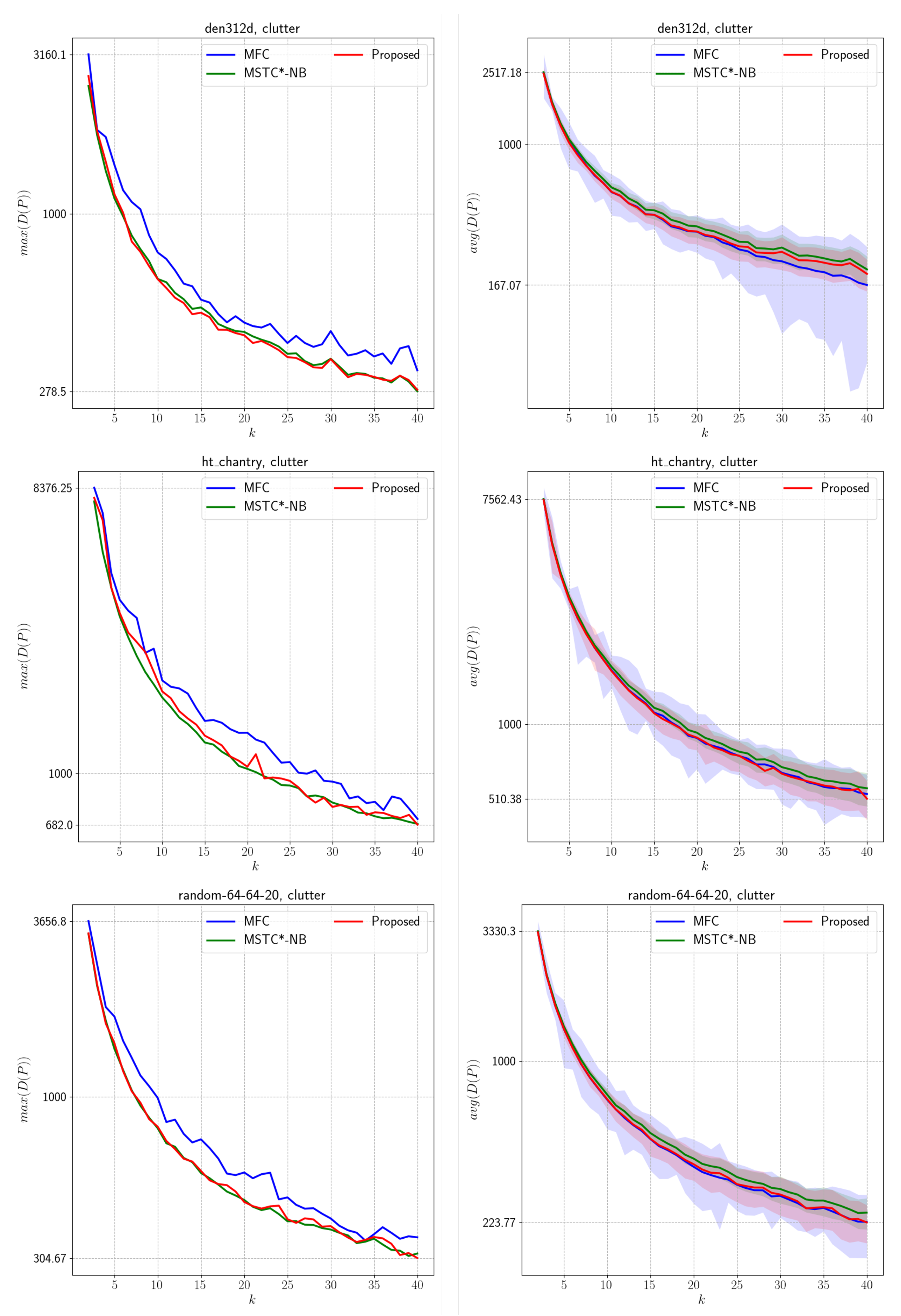
The evaluation results on grid graphs are summarized in

Table 2. Comparison of maximum path lengths on grid graphs. Bold indicates the minimum path length among methods for each k.

Type	Graph	Method	k
			2	5	10	20	30	40
arbitrary	den312d	MFC	3092	1282	780	501	372	278
		MSTC*-NB	2580	1114	677	442	367	331
		Proposed	2654	1110	628	387	330	275
	ht_chantry	MFC	8285	3636	2259	1394	1019	818
		MSTC*-NB	7627	3239	1782	1056	820	725
		Proposed	7744	3230	1692	1013	766	664
	random-64-64-20	MFC	3653	1700	968	571	439	340
		MSTC*-NB	3361	1415	780	486	373	331
		Proposed	3287	1423	770	465	354	315
clutter	den312d	MFC	3160	1424	758	457	430	324
		MSTC*-NB	2518	1119	626	427	352	279
		Proposed	2701	1153	625	417	351	282
	ht_chantry	MFC	8376	3634	1997	1352	940	712
		MSTC*-NB	7563	3213	1759	1033	804	686
		Proposed	7767	3295	1839	1050	778	682
	random-64-64-20	MFC	3656	1808	993	573	408	355
		MSTC*-NB	3331	1424	793	468	376	315
		Proposed	3341	1489	803	461	385	305

. In general, under arbitrary settings, our algorithm shows improved performance over the baselines across most graphs. An exception is observed in den312d and ht_chantry when $k=2$, where the result falls short of that of MSTC*-NB by approximately 4%. In clutter, the distance is overall higher than in arbitrary conditions. Moreover, as the complexity of the graph increases, specifically in random-64-64-20, the efficiency degrades by around 7%. We also report the standard deviations of each algorithm in the grid environment in

Table 3. Comparison of standard deviations of path lengths on grid graphs. Bold indicates the minimum deviation among methods for each k.

Type	Graph	Method	k
			2	5	10	20	30	40
arbitrary	den312d	MFC	599	191	153	83	73	42
		MSTC*-NB	25	33	48	50	49	50
		Proposed	203	84	53	43	47	39
	ht_chantry	MFC	760	313	373	266	169	135
		MSTC*-NB	17	60	73	84	82	88
		Proposed	268	146	74	94	78	77
	random-64-64-20	MFC	352	315	210	97	73	55
		MSTC*-NB	15	28	37	34	34	36
		Proposed	13	82	59	46	44	42
clutter	den312d	MFC	676	296	140	77	136	105
		MSTC*-NB	1	39	36	46	50	37
		Proposed	232	92	47	49	53	39
	ht_chantry	MFC	850	290	237	215	159	103
		MSTC*-NB	1	60	70	74	81	84
		Proposed	264	214	161	96	80	90
	random-64-64-20	MFC	353	408	167	108	52	64
		MSTC*-NB	1	33	38	32	38	35
		Proposed	43	102	62	54	51	39

. The proposed algorithm exhibits larger deviations than MSTC*-NB when the number of agents is small. Additionally, it shows higher values in cluttered environments. However, as k increases, the values converge to those of the baseline. Nevertheless, these results demonstrate that our method remains effective even in grid environments. The results for all tested values of k are reported in Figure A1 and Figure A2.

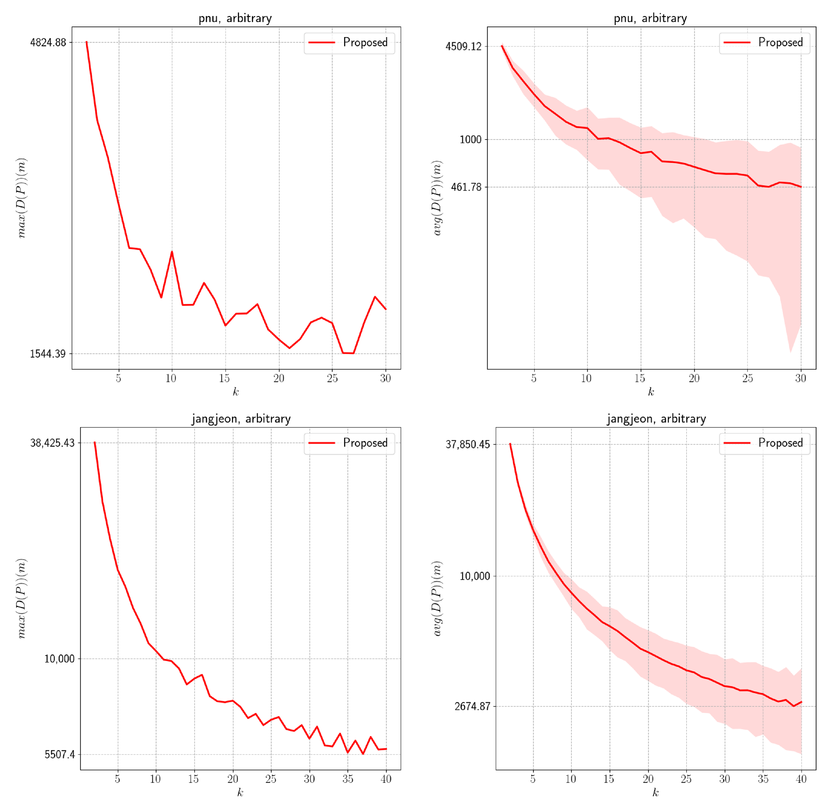
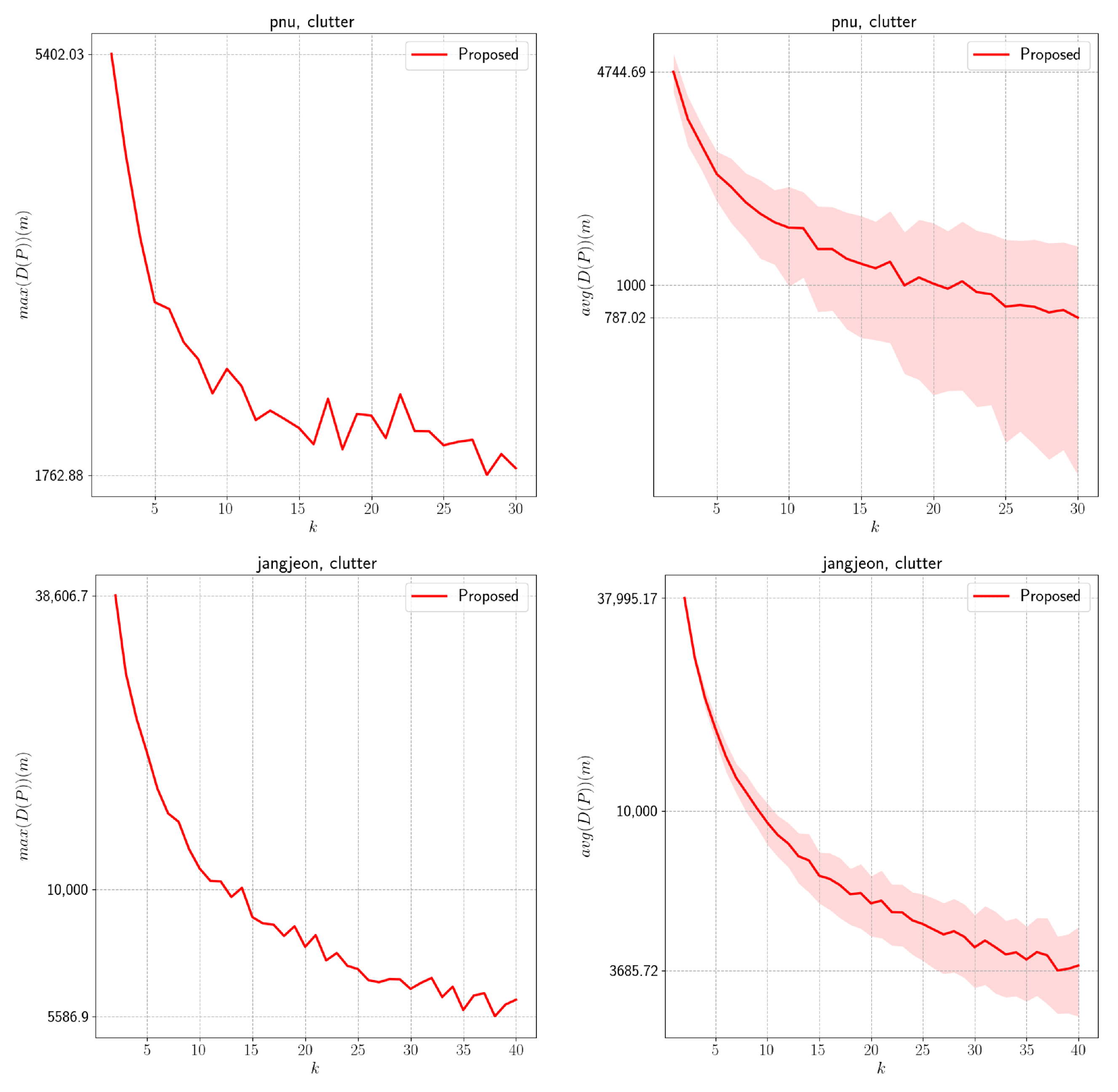
The results for non-grid graphs are presented in

Table 4. Comparison of runtime (s) on grid graphs. Bold indicates the minimum runtime among methods for each k.

Type	Graph	Method	k
			2	5	10	20	30	40
arbitrary	den312d	MFC	13.1	13.8	12.6	14.3	17.8	18.8
		MSTC*-NB	0.14	0.15	0.21	0.29	0.41	0.49
		Proposed	5.2	3.4	3.1	2.2	3.3	5
	ht_chantry	MFC	142.8	197.8	168.6	115.6	171.8	155.9
		MSTC*-NB	0.46	0.84	1.03	1.08	1.84	1.77
		Proposed	6.9	18.3	17.5	14.1	17.3	15.5
	random-64-64-20	MFC	28.5	42.4	45.4	54	56.1	58.7
		MSTC*-NB	0.2	0.34	0.45	0.65	0.81	0.91
		Proposed	1.8	2.6	2.1	3.4	4.4	6
clutter	den312d	MFC	27.2	23.3	28.2	41.2	56	57.2
		MSTC*-NB	0.24	0.26	0.32	0.61	0.76	0.71
		Proposed	6.2	3.6	3.9	3.8	4.5	4.6
	ht_chantry	MFC	223	228.7	239	169.1	241.4	217.9
		MSTC*-NB	0.74	0.96	1.16	1.05	1.87	1.82
		Proposed	8.9	23.5	17.5	17.3	16.8	19.1
	random-64-64-20	MFC	46.7	42.7	47.1	60.1	68.7	57.7
		MSTC*-NB	0.31	0.34	0.44	0.63	0.93	0.73
		Proposed	2.1	3.4	3.2	3.8	4.8	5.8

and

Table 5. Comparison of runtime (s) on non-grid graphs.

Type	Graph	Method	k
			2	5	10	20	30	40
arbitrary	pnu	Proposed	0.05	0.07	0.1	0.15	0.34
	jangjeon		20.5	20.5	18.6	16.5	13.9	16.4
clutter	pnu		0.05	0.08	0.1	0.15	0.36
	jangjeon		27.5	18.6	19.6	18	18.3	18.6

. As k increases, the generated paths become more distributed across all environments. Moreover, similarly to the grid case, clutter yields longer paths. However, as indicated in Figure A3 and Figure A4, as the number of agents increases, the path generation process becomes unstable. We will discuss the causes of these degradations and instabilities in the Conclusions.

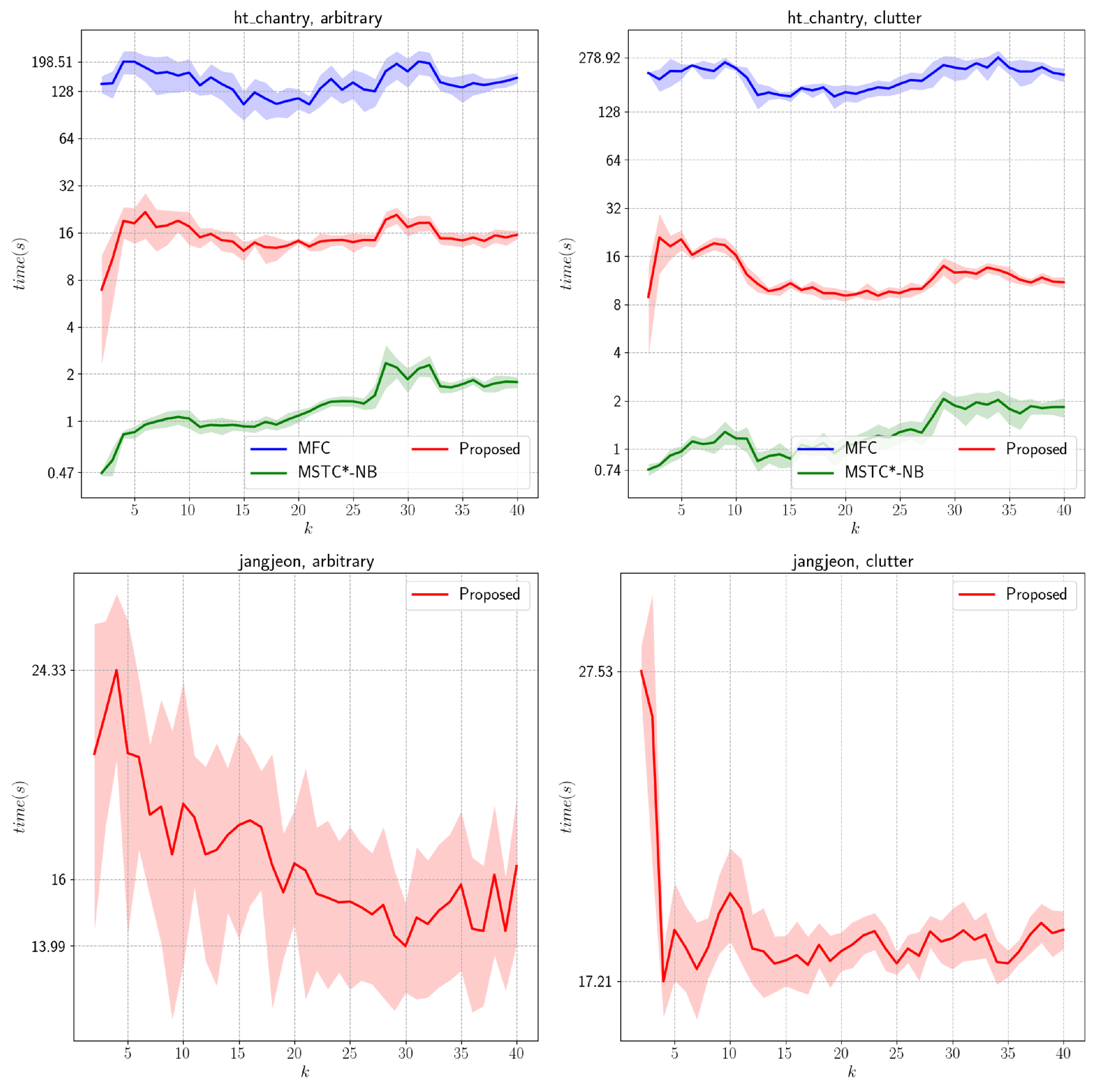
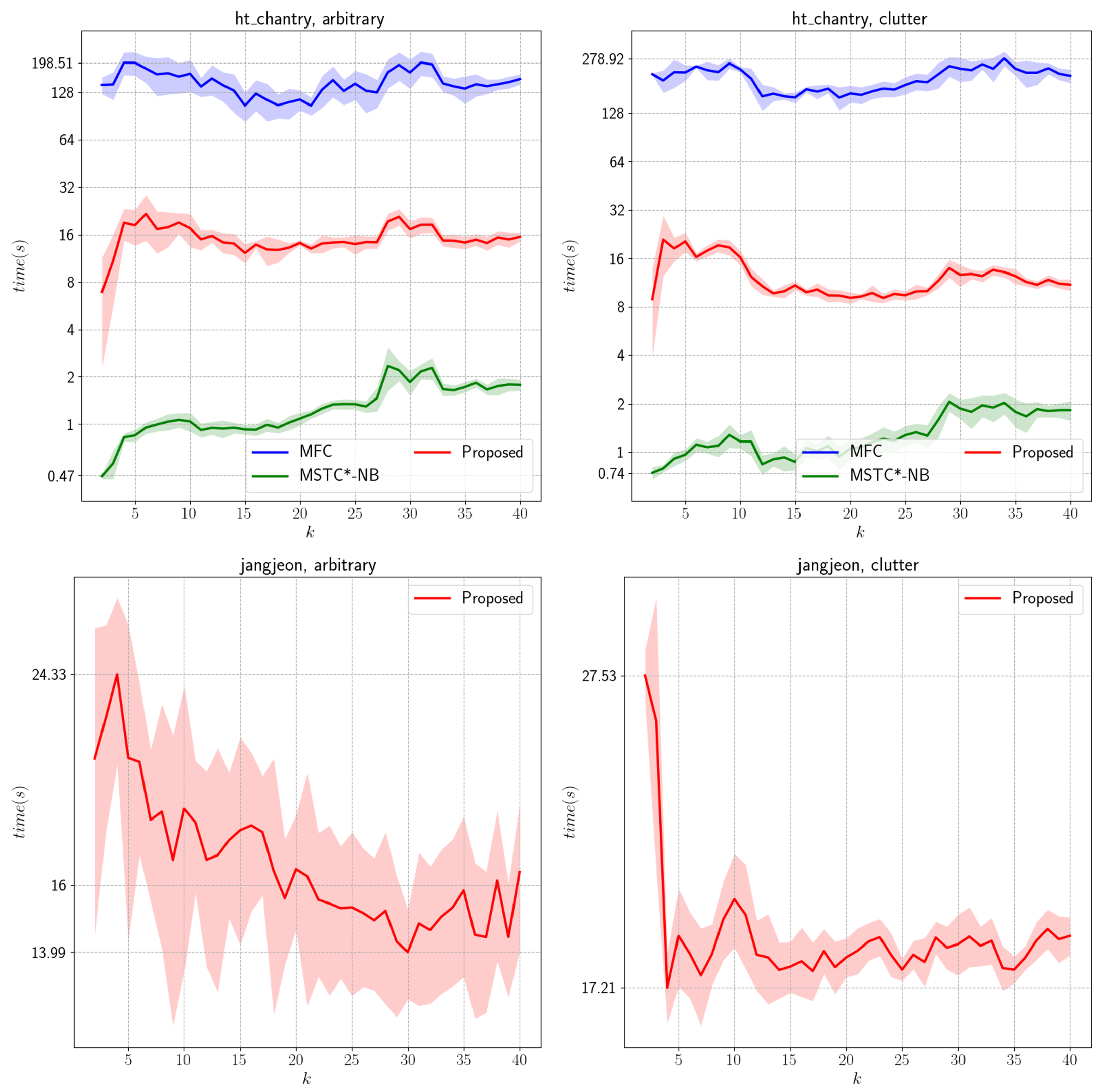
The runtime comparison of the algorithms is given in Table 6 and Table 7, and we present the results for ht_chantry and jangjeon in Figure 9. In these cases, the proposed algorithm completed execution in under one minute. Compared to MFC, it operated more than 10 times faster, but it remained about eight times slower than MSTC*-NB. As the number of graph nodes increased, the execution time consistently grew. Increasing k had contrasting effects on the runtime, becoming longer in grid but shorter in non-grid environments. Moreover, the algorithm exhibited approximately 5% longer runtimes in cluttered conditions compared to arbitrary ones. This indicates that the execution time rises with increasing environmental complexity.

Figure 9. Comparison of runtime on grid graph (ht_chantry) and non-grid graph (jangjeon).

Figure 9. Comparison of runtime on grid graph (ht_chantry) and non-grid graph (jangjeon).

Table 6. Comparison of maximum path lengths on non-grid graphs.

Type	Graph	Method	k
			2	5	10	20	30	40
arbitrary	pnu	Proposed	4824	2666	2240	1625	1816
	jangjeon		38,425	17,364	10,468	7680	6060	5682
clutter	pnu		5402	2791	2337	2064	1794
	jangjeon		38,606	18,762	11,010	7867	6335	6027

Table 6. Comparison of maximum path lengths on non-grid graphs.

Type	Graph	Method	k
			2	5	10	20	30	40
arbitrary	pnu	Proposed	4824	2666	2240	1625	1816
	jangjeon		38,425	17,364	10,468	7680	6060	5682
clutter	pnu		5402	2791	2337	2064	1794
	jangjeon		38,606	18,762	11,010	7867	6335	6027

Table 7. Comparison of standard deviations of path lengths on non-grid graphs.

Type	Graph	Method	k
			2	5	10	20	30	40
arbitrary	pnu	Proposed	316	393	484	398	412
	jangjeon		575	987	1256	1158	1030	1140
clutter	pnu		657	404	528	562	538
	jangjeon		611	1243	1202	1045	956	1035

Table 7. Comparison of standard deviations of path lengths on non-grid graphs.

Type	Graph	Method	k
			2	5	10	20	30	40
arbitrary	pnu	Proposed	316	393	484	398	412
	jangjeon		575	987	1256	1158	1030	1140
clutter	pnu		657	404	528	562	538
	jangjeon		611	1243	1202	1045	956	1035

6.3. Ablation Study

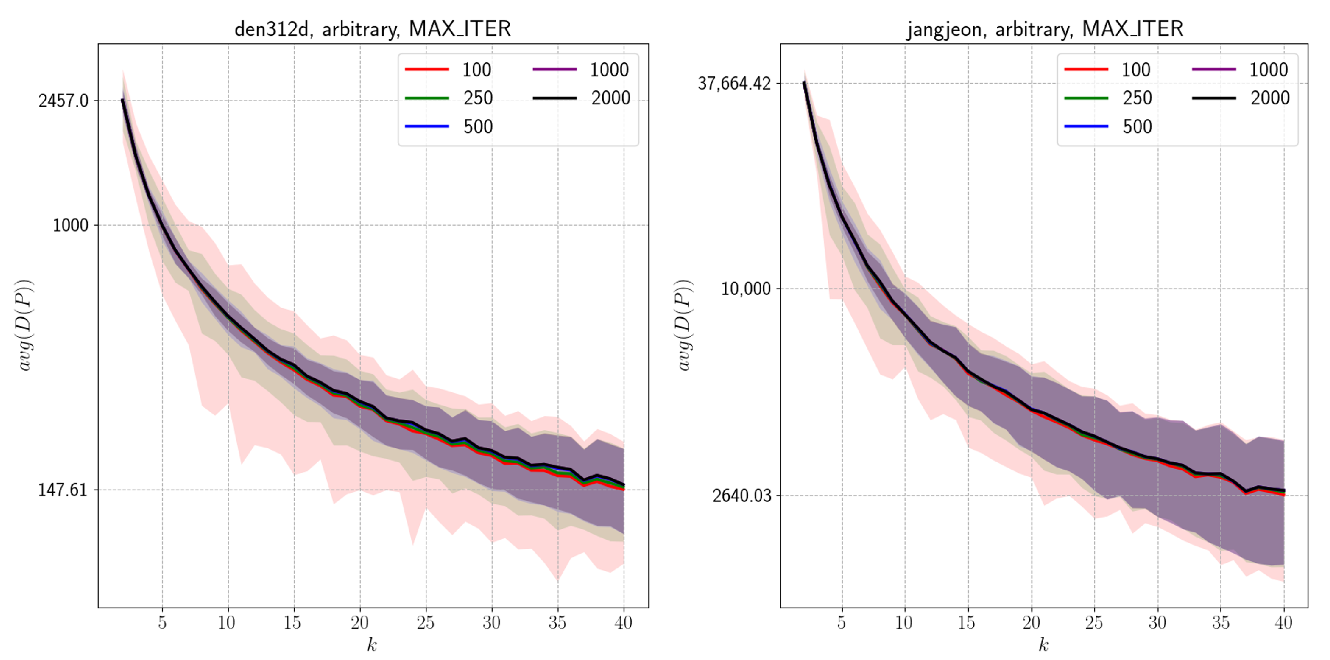
We conducted a comparative analysis of the proposed algorithm under both non-grid and grid environments by varying two primary parameters. For MAX_ITER, we employed values of 100, 250, 500, 1000, and 2000, while setting THRESHOLD = 0.005. The corresponding results are presented in Figure 10 and Table 8. With respect to the maximum path length, it became shorter with more iterations. However, over 1000 iterations, no significant improvement was observed. As shown in Figure 11 and Table 9, a similar pattern was found for the deviation, indicating that the algorithm operates more stably as the number of iterations increases.

Table 8. Comparison of maximum path lengths with respect to MAX_ITER. Bold indicates the minimum path length among methods for each k.

Type	Graph	MAX_ITER	k
			2	5	10	20	30	40
arbitrary	den312d	100	3089	1562	1045	561	429	305
		250	2926	1329	741	430	340	292
		500	2711	1143	646	402	343	299
		1000	2656	1099	635	394	343	299
		2000	2656	1102	631	394	343	299
	jangjeon	100	41,206	23,802	12,415	7869	6256	5837
		250	40,509	20,601	11,130	7060	6129	5769
		500	39,763	18,033	10,793	7019	6124	5725
		1000	38,044	17,240	10,630	6983	6119	5725
		2000	37,990	17,235	10,611	6983	6119	5725

Table 8. Comparison of maximum path lengths with respect to MAX_ITER. Bold indicates the minimum path length among methods for each k.

Type	Graph	MAX_ITER	k
			2	5	10	20	30	40
arbitrary	den312d	100	3089	1562	1045	561	429	305
		250	2926	1329	741	430	340	292
		500	2711	1143	646	402	343	299
		1000	2656	1099	635	394	343	299
		2000	2656	1102	631	394	343	299
	jangjeon	100	41,206	23,802	12,415	7869	6256	5837
		250	40,509	20,601	11,130	7060	6129	5769
		500	39,763	18,033	10,793	7019	6124	5725
		1000	38,044	17,240	10,630	6983	6119	5725
		2000	37,990	17,235	10,611	6983	6119	5725

Table 9. Comparison of standard deviations of path lengths with respect to MAX_ITER. Bold indicates the minimum deviation among methods for each k.

Type	Graph	MAX_ITER	k
			2	5	10	20	30	40
arbitrary	den312d	100	638	390	313	122	88	61
		250	476	224	135	77	58	49
		500	254	108	65	49	48	46
		1000	198	76	53	48	47	46
		2000	198	73	52	48	47	46
	jangjeon	100	3606	6258	2386	1591	1137	1129
		250	2874	3511	1494	1210	1022	1031
		500	2099	1675	1216	1093	1034	1031
		1000	391	1020	1174	1084	1036	1031
		2000	340	1003	1199	1086	1036	1031

Table 9. Comparison of standard deviations of path lengths with respect to MAX_ITER. Bold indicates the minimum deviation among methods for each k.

Type	Graph	MAX_ITER	k
			2	5	10	20	30	40
arbitrary	den312d	100	638	390	313	122	88	61
		250	476	224	135	77	58	49
		500	254	108	65	49	48	46
		1000	198	76	53	48	47	46
		2000	198	73	52	48	47	46
	jangjeon	100	3606	6258	2386	1591	1137	1129
		250	2874	3511	1494	1210	1022	1031
		500	2099	1675	1216	1093	1034	1031
		1000	391	1020	1174	1084	1036	1031
		2000	340	1003	1199	1086	1036	1031

Figure 10. Comparison of runtime with respect to MAX_ITER on den312d and jangjeon.

Figure 10. Comparison of runtime with respect to MAX_ITER on den312d and jangjeon.

Figure 11. Comparison of mean and standard deviation of path length with respect to MAX_ITER on den312d and jangjeon.

Figure 11. Comparison of mean and standard deviation of path length with respect to MAX_ITER on den312d and jangjeon.

To further examine the impact of THRESHOLD on performance, we tested values of 0.005 (0.5%), 0.01 (1%), 0.03 (3%), 0.05 (5%), and 0.1 (10%), while fixing MAX_ITER = 1000. As summarized in

Table 10. Comparison of maximum path lengths with respect to THRESHOLD. Bold indicates the minimum path length among methods for each k.

Type	Graph	THRESHOLD	k
			2	5	10	20	30	40
arbitrary	den312d	0.005	2668	1092	633	393	338	293
		0.01	2668	1094	634	393	338	294
		0.03	2668	1110	639	391	337	296
		0.05	2668	1119	642	390	337	295
		0.1	2689	1102	650	383	329	294
	jangjeon	0.005	38,219	17,526	10,465	7630	6563	5893
		0.01	38,280	17,535	10,472	7645	6563	5893
		0.03	38,449	17,527	10,490	7570	6561	5893
		0.05	38,487	17,522	10,524	7539	6561	5893
		0.1	38,748	18,117	10,521	7623	6528	5925

, the results show that higher threshold values led to approximately a 5% difference in the maximum path length when k was relatively small. However, this difference diminished as k increased.

The impact of the parameters on the runtime was evaluated, as presented in Figure 12. For MAX_ITER, the runtime increased as the parameter value increased. At low values of k, MAX_ITER = 2000 took approximately four times longer than MAX_ITER = 100. This effect became more pronounced with a larger k, where the runtime difference reached up to nine times. In contrast, for THRESHOLD, smaller values resulted in longer execution times.

7. Discussion

We present an offline MCPP algorithm for non-grid graphs. We employ a graph-adapted K-means method and modify its weights based on decomposing the path into initial and traversal paths. In this process, we explain the isolated component and local minima problems. To mitigate these issues, we introduce a merge step and cluster propagation via a cluster-level graph. Finally, paths are generated using STC and WHCA*. Through comparisons with prior work (MFC, MSTC*), we demonstrate that our algorithm works effectively on both grid and non-grid environments.

However, we observed degraded performance when the number of agents was small or the complexity was high. We attribute these outcomes to two primary limitations of the proposed algorithm. First, the optimally distributed traversal distance $d^{*}$ was designed for STC, and it is not directly applicable to weighted graphs. Determining the STC lengths of large clusters in weighted environments is challenging and often yields misleading results. As a result, when k is small, inaccuracies may arise, potentially yielding incorrect paths. We expect this problem to be mitigated by leveraging techniques for approximating the total weight of a minimum spanning tree [39]. Another limitation occurs in the merge step, where centroid shifts cause discrepancies between the estimated and actual initial path lengths. This effect is particularly pronounced in cluttered environments and accounts for the instability observed in the evaluation. We anticipate that the periodic recomputation of the initial path with bipartite graph matching will alleviate this issue.

The applicability of non-grid MCPP has significant implications for the design of interactive experiences in VR/AR environments. In particular, establishing a foundation that enables multiple agents to efficiently explore spaces and act cooperatively would enhance both the realism and the utility of immersive content. Furthermore, this study demonstrates the capability to explore paths within digital twins represented through diverse data structures. Non-grid graphs are well suited to represent environments where movement between adjacent cells is constrained. For example, when an agent travels by vehicle on a road, traffic regulations may impose directional restrictions on movement. These limitations are difficult to model with grid-based cells but can be represented easily via edges in non-grid graphs. Therefore, the proposed method can be applied to scenarios involving structured digital twins that can be used for urban, pedestrian-driven citizen science investigations or the vehicle-based monitoring of road networks. These contributions are expected to play a pivotal role in advancing large-scale multi-user virtual simulations, education and training systems, and intelligent collaborative virtual environments.

References

1. Nguyen, H.; Hussein, A.; Garratt, M.A.; Abbass, H.A. Swarm Metaverse for Multi-Level Autonomy Using Digital Twins. Sensors 2023, 23, 4892. [Google Scholar] [CrossRef]
2. Sharma, A.; Kosasih, E.; Zhang, J.; Brintrup, A.; Calinescu, A. Digital Twins: State of the art theory and practice, challenges, and open research questions. J. Ind. Inf. Integr. 2022, 30, 100383. [Google Scholar] [CrossRef]
3. Denk, M.; Bickel, S.; Steck, P.; Götz, S.; Völkl, H.; Wartzack, S. Generating Digital Twins for Path-Planning of Autonomous Robots and Drones Using Constrained Homotopic Shrinking for 2D and 3D Environment Modeling. Appl. Sci. 2022, 13, 105. [Google Scholar] [CrossRef]
4. Ahmed, M.F.; Maragliano, M.; Frémont, V.; Recchiuto, C.T. Efficient Multi-robot Active SLAM. J. Intell. Robot. Syst. 2025, 111, 64. [Google Scholar] [CrossRef]
5. Zhang, S.; Zhang, W.; Liu, C. Model-based Multi-UAV path planning for high-quality 3D reconstruction of buildings. Int. Arch. Photogramm. Remote. Sens. Spat. Inf. Sci. 2023, 48, 1923–1928. [Google Scholar] [CrossRef]
6. Ivić, S.; Crnković, B.; Grbčić, L.; Matleković, L. Multi-UAV trajectory planning for 3D visual inspection of complex structures. Autom. Constr. 2023, 147, 104709. [Google Scholar] [CrossRef]
7. Xiong, T.; Liu, F.; Liu, H.; Ge, J.; Li, H.; Ding, K.; Li, Q. Multi-Drone Optimal Mission Assignment and 3D Path Planning for Disaster Rescue. Drones 2023, 7, 394. [Google Scholar] [CrossRef]
8. Luna, M.A.; Isaac, M.S.A.; Ragab, A.R.; Cervera, P.C.; Peña, P.F.; González, M.M. Fast Multi-UAV Path Planning for Optimal Area Coverage in Aerial Sensing Applications. Sensors 2022, 22, 2297. [Google Scholar] [CrossRef]
9. Huang, X.; Sun, M.; Zhou, H.; Liu, S. A multi-robot coverage path planning algorithm for the environment with multiple land cover types. IEEE Access 2020, 8, 198101–198117. [Google Scholar] [CrossRef]
10. Collins, L.; Ghassemi, P.; Esfahani, E.T.; Doermann, D.; Dantu, K.; Chowdhury, S. Scalable Coverage Path Planning of Multi-Robot Teams for Monitoring Non-Convex Areas. In Proceedings of the 2021 IEEE International Conference on Robotics and Automation (ICRA), Xi’an, China, 30 May–5 June 2021; Institute of Electrical and Electronics Engineers Inc.: New York, NY, USA, 2021; pp. 7393–7399. [Google Scholar] [CrossRef]
11. Nigam, N.; Bieniawski, S.; Kroo, I.; Vian, J. Control of multiple UAVs for persistent surveillance: Algorithm and flight test results. IEEE Trans. Control. Syst. Technol. 2012, 20, 1236–1251. [Google Scholar] [CrossRef]
12. Botteghi, N.; Kamilaris, A.; Sinai, L.; Sirmacek, B. Multi-Agent Path Planning of Robotic Swarms in Agricultural Fields. Copernic. Gmbh 2020, 5, 361–368. [Google Scholar] [CrossRef]
13. Almadhoun, R.; Taha, T.; Seneviratne, L.; Zweiri, Y. A survey on multi-robot coverage path planning for model reconstruction and mapping. SN Appl. Sci. 2019, 1, 847. [Google Scholar] [CrossRef]
14. Galceran, E.; Campos, R.; Palomeras, N.; Ribas, D.; Carreras, M.; Ridao, P. Coverage Path Planning with Real-time Replanning and Surface Reconstruction for Inspection of Three-dimensional Underwater Structures using Autonomous Underwater Vehicles. J. Field Robot. 2015, 32, 952–983. [Google Scholar] [CrossRef]
15. Bouman, A.; Ott, J.; Kim, S.K.; Chen, K.; Kochenderfer, M.J.; Lopez, B.; Agha-Mohammadi, A.A.; Burdick, J. Adaptive Coverage Path Planning for Efficient Exploration of Unknown Environments. In Proceedings of the 2022 IEEE/RSJ International Conference on Intelligent Robots and Systems (IROS), Kyoto, Japan, 23–27 October 2022; Institute of Electrical and Electronics Engineers Inc.: New York, NY, USA, 2022; pp. 11916–11923. [Google Scholar] [CrossRef]
16. Nair, V.G.; Dileep, M.V.; Guruprasad, K.R. Robust Online Multi-Robot Simultaneous Exploration and Coverage Path Planning. IEEE Access 2024, 12, 72990–73003. [Google Scholar] [CrossRef]
17. Tang, J.; Gao, Y.; Lam, T.L. Learning to Coordinate for a Worker-Station Multi-Robot System in Planar Coverage Tasks. IEEE Robot. Autom. Lett. 2022, 7, 12315–12322. [Google Scholar] [CrossRef]
18. Wang, Z.; Zhao, X.; Zhang, J.; Yang, N.; Wang, P.; Tang, J.; Zhang, J.; Shi, L. APF-CPP: An Artificial Potential Field Based Multi-robot Online Coverage Path Planning Approach. IEEE Robot. Autom. Lett. 2024, 9, 9199–9206. [Google Scholar] [CrossRef]
19. Ann, S.; Kim, Y.; Ahn, J. Area allocation algorithm for multiple UAVs area coverage based on clustering and graph method. IFAC-PapersOnLine 2015, 28, 204–209. [Google Scholar] [CrossRef]
20. Tang, Y.; Zhou, R.; Sun, G.; Di, B.; Xiong, R. A Novel Cooperative Path Planning for Multirobot Persistent Coverage in Complex Environments. IEEE Sens. J. 2020, 20, 4485–4495. [Google Scholar] [CrossRef]
21. Gabriely, Y.; Rimon, E. Spanning-tree based coverage of continuous areas by a mobile robot. Ann. Math. Artif. Intell. 2001, 31, 1927–1933. [Google Scholar] [CrossRef]
22. Jimenez, P.A.; Shirinzadeh, B.; Nicholson, A.; Alici, G. Optimal area covering using genetic algorithms. In Proceedings of the 2007 IEEE/ASME International Conference on Advanced Intelligent Mechatronics, Zurich, Switzerland, 4–7 September 2007; pp. 1–5. [Google Scholar] [CrossRef]
23. Sieranoja, S.; Fränti, P. Adapting k-means for graph clustering. Knowl. Inf. Syst. 2022, 64, 115–142. [Google Scholar] [CrossRef]
24. Hazon, N.; Kaminka, G. Redundancy, Efficiency and Robustness in Multi-Robot Coverage. In Proceedings of the 2005 IEEE International Conference on Robotics and Automation, Barcelona, Spain, 18–22 April 2005; pp. 735–741. [Google Scholar] [CrossRef]
25. Fazli, P.; Davoodi, A.; Pasquier, P.; Mackworth, A.K. Complete and robust cooperative robot area coverage with limited range. In Proceedings of the 2010 IEEE/RSJ International Conference on Intelligent Robots and Systems, Taipei, Taiwan, 18–22 October 2010; Volume 10, pp. 5577–5582. [Google Scholar] [CrossRef]
26. Majeed, A.; Hwang, S.O. A multi-objective coverage path planning algorithm for uavs to cover spatially distributed regions in urban environments. Aerospace 2021, 8, 343. [Google Scholar] [CrossRef]
27. Christofides, N. Worst-Case Analysis of a New Heuristic for the Travelling Salesman Problem. Oper. Res. Forum 2022, 3, 20. [Google Scholar] [CrossRef]
28. Hazon, N.; Mieli, F.; Kaminka, G. Towards robust on-line multi-robot coverage. In Proceedings of the 2006 IEEE International Conference on Robotics and Automation (ICRA 2006), Orlando, FL, USA, 15–19 May 2006; pp. 1710–1715. [Google Scholar] [CrossRef]
29. Zheng, X.; Jain, S.; Koenig, S.; Kempe, D. Multi-robot forest coverage. In Proceedings of the 2005 IEEE/RSJ International Conference on Intelligent Robots and Systems, Edmonton, AB, Canada, 2–6 August 2005; pp. 3852–3857. [Google Scholar] [CrossRef]
30. Tang, J.; Sun, C.; Zhang, X. MSTC*: Multi-robot Coverage Path Planning under Physical Constrain. In Proceedings of the 2021 IEEE International Conference on Robotics and Automation (ICRA), Xi’an, China, 30 May–5 June 2021; Volume 5, pp. 2518–2524. [Google Scholar] [CrossRef]
31. Lu, J.; Zeng, B.; Tang, J.; Lam, T.L.; Wen, J. TMSTC*: A Path Planning Algorithm for Minimizing Turns in Multi-Robot Coverage. IEEE Robot. Autom. Lett. 2023, 8, 5275–5282. [Google Scholar] [CrossRef]
32. Mo, W.; Lin, Z. MDSTC: A Dynamic Approach to Multi-Robot Coverage Path Planning. In Proceedings of the 2024 18th International Conference on Control, Automation, Robotics and Vision (ICARCV), Dubai, United Arab Emirates, 12–15 December 2024; Volume 12, pp. 1100–1105. [Google Scholar] [CrossRef]
33. Kapoutsis, A.C.; Chatzichristofis, S.A.; Kosmatopoulos, E.B. DARP: Divide Areas Algorithm for Optimal Multi-Robot Coverage Path Planning. J. Intell. Robot. Syst. 2017, 86, 663–680. [Google Scholar] [CrossRef]
34. Liu, Y.; Hu, J.; Dong, W. Decentralized Coverage Path Planning with Reinforcement Learning and Dual Guidance. arXiv 2022, arXiv:cs.RO/2210.07514. [Google Scholar] [CrossRef]
35. Ni, J.; Gu, Y.; Tang, G.; Ke, C.; Gu, Y. Cooperative Coverage Path Planning for Multi-Mobile Robots Based on Improved K-Means Clustering and Deep Reinforcement Learning. Electronics 2024, 13, 944. [Google Scholar] [CrossRef]
36. Silver, D. Cooperative Pathfinding. In Proceedings of the AAAI Conference on Artificial Intelligence and Interactive Digital Entertainment, Virtual, 11–15 October 2021; Volume 1, pp. 117–122. [Google Scholar] [CrossRef]
37. Stern, R.; Sturtevant, N.; Felner, A.; Koenig, S.; Ma, H.; Walker, T.; Li, J.; Atzmon, D.; Cohen, L.; Kumar, T.K.; et al. Multi-Agent Pathfinding: Definitions, Variants, and Benchmarks. Proc. Int. Symp. Comb. Search 2021, 10, 151–158. [Google Scholar] [CrossRef]
38. Treinish, M.; Carvalho, I.; Tsilimigkounakis, G.; Sá, N. rustworkx: A High-Performance Graph Library for Python. J. Open Source Softw. 2022, 7, 3968. [Google Scholar] [CrossRef]
39. Chazelle, B.; Rubinfeld, R.; Trevisan, L. Approximating the Minimum Spanning Tree Weight in Sublinear Time. SIAM J. Comput. 2005, 34, 1370–1379. [Google Scholar] [CrossRef]
Figure 1. Example environment represented as a graph. The grid graph (left) exhibits regular connections between adjacent vertices, whereas the non-grid graph (right) lacks such structural regularity.
Electronics 14 03921 g001
Figure 2. Example graph with two clusters. Each color of the vertices represents a distinct cluster.
Electronics 14 03921 g002
Figure 3. The overall path is divided into the initial path and the traversal path. s A denotes the starting vertex of agent A. p A i n i t refers to the path from agent A’s initial point to the cluster A. p A t r a v e r s e represents the traversal path that visits all vertices within cluster A. Each color of the vertices represents a distinct cluster and star indicates agent’s initial position.
Electronics 14 03921 g003
Figure 4. Grid graph G (left) and its corresponding bipartite graph representation B (right). In the grid graph, SA and SB denote the initial vertices of agents A and B, respectively, and are shown as stars on the vertices. Each color of the vertices represents a distinct cluster. In the bipartite graph, vertices A and B represent agents A and B, while X and Y denote clusters X and Y, respectively. The numbers on the edges indicate the path lengths from each agent’s initial vertex to each cluster.
Electronics 14 03921 g004
Figure 5. Isolated component generated in the K-step (left middle) and the merged result from the M-step (right). Each color of the vertices represents a distinct cluster.
Electronics 14 03921 g005
Figure 6. Issues during cluster updates. Each color of the vertices represents a distinct cluster. (a,b) shows graph with k = 2 and k = 4. Given the current updating rule, (a,b) can be updated since there are adjacent vertices between the clusters (represented by a red cross in c). However, in (c), another cluster lies between the two clusters, requiring updates to pass through them.
Electronics 14 03921 g006
Figure 8. Graphs used for evaluation, with the numbers of vertices and edges. The upper graph has a grid structure, while the lower graph has a non-grid structure.
Electronics 14 03921 g008
Figure 12. Comparison of runtime with respect to MAX_ITER and THRESHOLD on den312d and jangjeon.
Electronics 14 03921 g012