Low-Rank Matrix Completion via Nonconvex Rank Approximation for IoT Network Localization

Abstract

Accurate node localization is essential for many Internet of Things (IoT) applications. However, incomplete and noisy distance measurements often degrade the reliability of the Euclidean Distance Matrix (EDM), which is critical for range-based localization. To address this issue, a Low-Rank Matrix Completion approach based on nonconvex rank approximation (LRMCN) is proposed to recover the true EDM. First, the observed EDM is decomposed into a low-rank matrix representing the true distances and a sparse matrix capturing noise. Second, a nonconvex surrogate function is used to approximate the matrix rank, while the $l_1$-norm is utilized to model the sparsity of the noise component. Third, the resulting optimization problem is solved using the Alternating Direction Method of Multipliers (ADMMs). This enables accurate recovery of a complete and denoised EDM from incomplete and corrupted measurements. Finally, relative node locations are estimated using classical multi-dimensional scaling, and absolute coordinates are determined based on a small set of anchor nodes with known locations. The experimental results show that the proposed method achieves superior performance in both matrix completion and localization accuracy, even in the presence of missing and corrupted data.

1. Introduction

The Internet of Things (IoT) has attracted increasing attention due to its wide range of applications, including environmental monitoring, smart healthcare, industrial automation, and intelligent surveillance [1]. In such applications, large-scale Wireless Sensor Networks (WSNs) are widely deployed to collect environmental data such as temperature, humidity, air quality, and object movement [2]. To enable timely and context-aware responses, accurate location information of sensor nodes is essential, as key decisions such as fire detection, energy management, and emergency response are typically executed at a centralized data center [3,4].

Range-based localization is a widely used technique for determining node positions in WSNs, where pairwise distances are obtained through methods such as Received Signal Strength Indication (RSSI), Time of Arrival (ToA), Time Difference of Arrival (TDoA), and Angle of Arrival (AoA) [5,6]. These measurements form a Euclidean Distance Matrix (EDM), which provides the geometric constraints required by algorithms, including multilateration [7], Semi-definite Programming (SDP) [8], and multi-dimensional scaling (MDS) [9]. A complete EDM uniquely determines the relative node configuration up to rigid transformations, enabling absolute localization when aligned with anchor nodes [10]. Thus, sufficient and accurate distance measurements are essential for reliable positioning. Moreover, the EDM captures the intrinsic low-dimensional geometric structure of the network, which can be further exploited for both precise localization and robust topology recovery [11].

However, constructing a complete EDM requires measuring distances between all node pairs, which entails frequent communication and results in significant energy overhead [12]. In practical deployments, constraints such as limited battery life and restricted communication ranges often prevent the acquisition of full distance information, leading to incomplete EDMs and increased complexity in the localization process. In addition to data incompleteness, measurement inaccuracies are common due to environmental and hardware-related disturbances. Specifically, the collected distances are often contaminated by two dominant types of noise: Gaussian noise and outlier noise. Gaussian noise typically arises from sensor imprecision or computational errors and is modeled as zero-mean Gaussian-distributed perturbations [13]. Outlier noise, on the other hand, corresponds to sporadic large deviations from true values, often induced by non-line-of-sight conditions, multipath effects, hardware malfunction, or adversarial interference [14]. These imperfections result in an EDM that is not only incomplete but also noisy, posing significant challenges to robust and high-accuracy localization in WSNs and broader IoT applications.

To address the challenges of incomplete and noisy distance measurements in IoT network localization, this work proposes a Low-Rank Matrix Completion approach based on nonconvex rank approximation (LRMCN) for accurate EDM recovery and location estimation. Specifically, the observed EDM is modeled as the superposition of a low-rank matrix representing the true inter-node distances and a sparse matrix accounting for measurement noise and outliers. To recover the underlying structured EDM, a nonconvex surrogate is employed to approximate the matrix rank, while the ${\ell }_1$-norm regularization promotes sparsity in the noise component. The resulting optimization problem is efficiently solved using the Alternating Direction Method of Multipliers (ADMMs) [15], enabling accurate reconstruction of a complete and denoised EDM from incomplete and corrupted observations. Subsequently, relative node positions are derived via classical MDS, and absolute coordinates are determined with the assistance of a limited number of anchor nodes. Experimental evaluations confirm that the proposed method achieves high localization accuracy in scenarios with both missing and corrupted data.

The main contributions are summarized as follows:

• A novel formulation is proposed to decompose the observed EDM into a low-rank component representing true distances and a sparse component modeling measurement noise and outliers. This formulation enhances robustness under both missing and corrupted data.
• A nonconvex surrogate function is adopted to more accurately approximate the rank constraint, while the ${\ell }_1$-norm is used to enforce sparsity in the noise matrix. This enables more precise recovery of the underlying EDM structure.
• The resulting nonconvex and nonsmooth optimization problem is solved using an ADMM framework, which ensures stable convergence and computational efficiency.
• Reconstructed EDMs are converted into relative node positions via MDS, and absolute positions are obtained using a small number of anchor nodes, facilitating practical deployment.

The remainder of this paper is organized as follows. Section 2 reviews the related work. Section 3 describes the ranging model and formulates the problem. Section 4 details the proposed LRMCN algorithm and the corresponding localization method. Section 5 presents the simulation results and analysis. Section 6 concludes the paper.

2. Related Works

EDM serves as a fundamental representation of pairwise node distances in wireless networks and underpins most range-based localization techniques [16]. In practice, EDMs are typically derived from various distance measurements such as RSSI, ToA, TDoA, and AoA. However, due to limitations in sensing and communication capabilities, the resulting EDM is often incomplete and contaminated by noise, which significantly hinders accurate localization.

In response to this challenge, Low-Rank Matrix Completion (LRMC) has emerged as a promising solution by exploiting the intrinsic low-rank characteristics of ideal EDMs. Several representative LRMC algorithms have been applied to EDM recovery, including Exact Completion Solution (ECS) [17], Singular Value Thresholding (SVT) [18], and Augmented Lagrange Multiplier (ALM) [19]. While ECS can achieve exact recovery when sufficient clean distance data is available, its performance deteriorates under noisy conditions [17]. Alternatively, SVT and related methods formulate EDM completion as a low-rank optimization problem [8,18]. These approaches typically involve iterative singular-value decomposition and thresholding, which may result in slow convergence and limited recovery accuracy, especially when the data is highly corrupted.

One widely adopted strategy for LRMC is to relax the rank minimization problem using the nuclear norm, which serves as the tightest convex surrogate for the nonconvex rank function [20,21]. This approach transforms the original NP-hard optimization problem into a convex formulation, enabling more tractable solutions with theoretical recovery guarantees under certain conditions. Several algorithms based on nuclear norm minimization have been proposed and successfully applied to distance matrix completion tasks [13,15,22,23]. To address the issue of incomplete and noisy distance data in WSNs, Xiao et al. [14] proposed LoMaC, a noise-tolerant localization method that formulates EDM completion as a norm-regularized matrix completion problem. Leveraging Frobenius and $l_1$ norms and solving via an ADMM-based algorithm, LoMaC achieves robust distance recovery, followed by node localization through multi-dimensional scaling.

Despite the theoretical appeal and algorithmic tractability of nuclear norm minimization, its performance in practical applications such as IoT localization is often limited. This is primarily due to the fact that the nuclear norm penalizes all singular values uniformly, which may not align well with the actual structure of the underlying matrix [24]. In many real-world scenarios, especially those involving incomplete and noisy EDMs, the true rank is relatively low but the singular values decay gradually rather than abruptly. As a result, nuclear norm minimization tends to over-regularize the larger singular values, leading to suboptimal recovery of the distance matrix and degraded localization accuracy.

To address these limitations, recent studies have shifted toward nonconvex rank approximation techniques [24,25]. These approaches replace the nuclear norm with nonconvex surrogate functions such as the truncated nuclear norm [22], Schatten-p norm [23], and Logarithmic norm [26], which better preserve dominant singular values while still promoting low-rank structure. Although nonconvex formulations are generally more challenging to optimize, advances in numerical optimization techniques, including the Alternating Direction Method of Multipliers (ADMMs) [15] and proximal gradient methods [27], have enabled efficient and scalable solvers for such models. Empirical results have demonstrated that nonconvex methods can significantly improve matrix recovery quality, especially in settings with high levels of noise or severe data incompleteness.

3. System Model

Consider a network consisting of N sensor nodes randomly deployed in a d-dimensional monitoring region, where the positions of M anchor nodes equipped with GPS are known, and the remaining $N-M$ nodes (referred to as normal nodes) have unknown positions. Each node is assumed to have a communication radius R, enabling it to measure distances to neighboring nodes within range and transmit this information to a data center. Let ${\left\{{\mathbf{u}}_j\right\}}_{j=1}^M\in {\mathbb{R}}^d$ and ${\left\{{\mathbf{x}}_i\right\}}_{i=M+1}^N\in {\mathbb{R}}^d$ denote the coordinates of anchor nodes and normal nodes, respectively, where $d\in \left\{2,3\right\}$. For notational convenience, define the coordinate matrix as $\mathbf{Y}=\left[{\mathbf{u}}_1,\dots ,{\mathbf{u}}_M,{\mathbf{x}}_{M+1},\dots ,{\mathbf{x}}_N\right]\in {\mathbb{R}}^{d\times N}$, and let $\mathbf{D}\in {\mathbb{R}}^{N\times N}$ represent the corresponding EDM, which can be formulated as

$${\mathbf{D}}_{ij}={\parallel {\mathbf{y}}_i-{\mathbf{y}}_j\parallel }_2,i,j=1,2,\dots ,N.$$

(1)

where ${\mathbf{y}}_i$ denotes the coordinates of node i. Then, ${\mathbf{D}}_{ij}={\parallel {\mathbf{y}}_i-{\mathbf{y}}_j\parallel }_2$ is the squared Euclidean distance between nodes i and j.

3.1. Ranging Model

This work focuses on an RSSI-based ranging model, which offers a cost-effective and hardware-friendly solution for distance measurement. Simulations were conducted under RSSI scenarios to evaluate the proposed localization method.

The RSSI-based ranging model estimates the distance between two nodes by analyzing the received signal strength. According to the $log$-normal shadowing path-loss model, the received power decays logarithmically with distance. The model is typically expressed as [6]

$$P_{ij}=P_0-10n_p{log}_{10}\left({\displaystyle \frac{d_{ij}}{d_0}}\right),$$

(2)

where $P_0$ is the received power at a reference distance $d_0$, and $n_p$ is the path-loss exponent.

In practice, the received signal is affected by additive Gaussian noise [28], as follows:

$${\tilde{P}}_{ij}=P_{ij}+q_{ij},q_{ij}\sim \mathcal{N}(0,{\sigma }^2),$$

(3)

Using the noisy signal strength ${\tilde{P}}_{ij}$, the estimated distance is computed as

$${\tilde{d}}_{ij}=d_0·{10}^{{\displaystyle \frac{P_0-{\tilde{P}}_{ij}}{10n_p}}},$$

(4)

Since the RSSI is inversely related to distance, its accuracy degrades over long ranges, and it is therefore only reliable within a limited communication radius.

It should be noted that, although our simulations adopt RSSI-based distance measurements, the proposed LRMCN framework is not limited to this specific modality. Since the essence of the problem lies in completing missing distance elements, the method can be similarly applied when the distance information is obtained through ToA, TDoA, or AoA techniques. Thus, the choice of RSSI in our experiments mainly serves to demonstrate the effectiveness of the algorithm, while extensions to other measurement modalities remain a promising direction for future work.

3.2. Problem Formulation

In typical range-based localization algorithms, if all pairwise distances are known, the locations of normal nodes can be accurately estimated using techniques such as MDS-MAP [29] or SDP [8]. However, due to energy constraints, limited communication range, and noise interference, it is often infeasible to acquire complete and accurate distance data, resulting in an incomplete and noisy EDM. This study aims to complete the partially observed EDM via the LRMC method as a critical step toward reliable IoT localization. To this end, we formulate the recovery of the structured EDM as an optimization problem based on the following objective function [30]:

$$\begin{array}{cc}\hfill & \underset{\mathbf{S}}{min}\mathrm{rank}\left(\mathbf{S}\right)\hfill \\ \hfill \mathrm{s}.\mathrm{t}.& P_{\mathrm{\Omega }}\left(\mathbf{S}\right)=P_{\mathrm{\Omega }}\left(\mathbf{D}\right)\hfill \end{array}$$

(5)

where $\mathbf{S}\in {\mathbb{R}}^{N\times N}$ denotes the sampled distance matrix. $\mathrm{\Omega }$ denotes the set of subscripts of known elements in the matrix $\mathbf{S}$, and $P_{\mathrm{\Omega }}$ represents the projection operator, which is defined as

$$P_{\mathrm{\Omega }}\left({\mathbf{D}}_{ij}\right)=\left\{\begin{array}{c}{\mathbf{D}}_{ij},\mathrm{if}\left(i,j\right)\in \mathrm{\Omega },\hfill \\ 0,\mathrm{if}\left(i,j\right)\notin \mathrm{\Omega }.\hfill \end{array}\right.$$

(6)

In real-world applications, the sampled matrices are usually corrupted by sparse noise. Accordingly, the relationship between the sampled distance matrix $\mathbf{S}$ and the complete distance matrix $\mathbf{D}$ is expressed as

$$P_{\mathrm{\Omega }}\left(\mathbf{S}\right)=P_{\mathrm{\Omega }}\left(\mathbf{D}+\mathbf{E}\right),$$

(7)

where $\mathbf{E}$ is the noise matrix, and $\mathbf{S}=\mathbf{D}+\mathbf{E}$.

When the given matrix satisfies the incoherence conditions proposed by Candès and Tao [21], the matrix completion problem can be addressed by recovering a low-rank matrix that approximates the underlying data. Moreover, incorporating sparsity-inducing norms helps mitigate the impact of noise [31]. By exploiting the low-rank property of noise-free EDMs and the sparsity of outlier noise [13], the observed matrix $\mathbf{S}$ can be modeled as the sum of a low-rank matrix $\mathbf{D}$ and a sparse noise matrix $\mathbf{E}$. Accordingly, the EDM reconstruction problem is formulated as

$$\begin{array}{c}\underset{\mathbf{D},\mathbf{E}}{min}\mathrm{rank}\left(\mathbf{D}\right)+\lambda {∥\mathbf{E}∥}_0\\ \mathrm{s}.\mathrm{t}.P_{\mathrm{\Omega }}\left(\mathbf{S}\right)=P_{\mathrm{\Omega }}\left(\mathbf{D}+\mathbf{E}\right).\end{array}$$

(8)

where $\lambda$ is a trade-off parameter balancing low-rank and sparsity terms.

4. Algorithm Development

4.1. Nonconvex Rank Approximation Based Matrix Completion

Directly solving the problem in Equation (8) is computationally intractable due to the nonconvexity of both the rank function and the $l_0$ norm, rendering the optimization NP-hard. A widely adopted strategy is to apply convex relaxation by substituting the rank function with the nuclear norm and the $l_0$ norm with the $l_1$ norm, thereby transforming Equation (8) into the following convex relaxation:

$$\begin{array}{c}\underset{\mathbf{D},\mathbf{E}}{min}{∥\mathbf{D}∥}_{\ast }+\lambda {∥\mathbf{E}∥}_1\\ \mathrm{s}.\mathrm{t}.P_{\mathrm{\Omega }}\left(\mathbf{S}\right)=P_{\mathrm{\Omega }}\left(\mathbf{D}+\mathbf{E}\right).\end{array}$$

(9)

To achieve a more accurate rank approximation and reduce computational complexity, a nonconvex rank approximation matrix reconstruction model is proposed based on the low-rank decomposition of matrices. Specifically, the complete distance matrix $\mathbf{D}\in {\mathbb{R}}^{N\times N}$ is approximated by the product of two low-rank matrices $\mathbf{U}\in {\mathbb{R}}^{N\times r}$ and $\mathbf{V}\in {\mathbb{R}}^{N\times r}$, i.e., $\mathbf{D}\approx \mathbf{U}{\mathbf{V}}^T$. The optimization problem is then formulated as

$$\begin{array}{c}\underset{\mathbf{U},\mathbf{V},\mathbf{E}}{min}{∥\mathbf{V}∥}_{\ast }+\lambda {∥\mathbf{E}∥}_1\hfill \\ \mathrm{s}.\mathrm{t}.P_{\mathrm{\Omega }}\left(\mathbf{S}\right)=P_{\mathrm{\Omega }}\left(\mathbf{U}{\mathbf{V}}^T+\mathbf{E}\right),\hfill \\ {\mathbf{U}}^T\mathbf{U}=\mathbf{I}.\hfill \end{array}$$

(10)

It is well known that the nuclear norm is not an ideal surrogate of the rank function, as it tends to over-penalize large singular values, requires expensive singular value decompositions, and is sensitive to noise contamination. To overcome these limitations, recent studies have introduced nonconvex rank surrogates [32]. Following this line, we adopt a matrix factorization strategy, which transforms Equation (8) into the smaller-scale optimization problem in Equation (10). This not only reduces computational overhead but also enables a more accurate and robust approximation of the intrinsic rank structure.

Further, the kernel norm of the matrix is relaxed using a nonconvex regular term based on the Laplace function, transforming the problem of Equation (10) into the following form:

$$\begin{array}{c}\underset{\mathbf{U},\mathbf{V},\mathbf{E}}{min}{∥\mathbf{V}∥}_{\gamma }+\lambda {∥\mathbf{E}∥}_1\hfill \\ \mathrm{s}.\mathrm{t}.P_{\mathrm{\Omega }}\left(\mathbf{S}\right)=P_{\mathrm{\Omega }}\left(\mathbf{U}{\mathbf{V}}^T+\mathbf{E}\right),\hfill \\ {\mathbf{U}}^T\mathbf{U}=\mathbf{I}.\hfill \end{array}$$

(11)

where ${∥\mathbf{V}∥}_{\gamma }={\displaystyle \sum _{i=1}^m}{\displaystyle \frac{\left(1+\gamma \right){\sigma }_i\left(\mathbf{V}\right)}{\gamma +{\sigma }_i\left(\mathbf{V}\right)}}$ is a nonconvex function [32], and ${\delta }_i$ denotes the singular value of $\mathbf{V}$ with $0<\gamma <1$. For ${∥\mathbf{V}∥}_{\gamma }$, it satisfies $\underset{\gamma \to 0}{lim}{∥\mathbf{V}∥}_{\gamma }=\mathrm{rank}\left(\mathbf{V}\right)$ and $\underset{\gamma \to \infty }{lim}{∥\mathbf{V}∥}_{\gamma }={∥\mathbf{V}∥}_{\ast }$ [33]. Moreover, for any $\mathbf{A}\in {\mathbb{R}}^{m\times m}$ and $\mathbf{B}\in {\mathbb{R}}^{m\times m}$, we have that ${∥\mathbf{V}∥}_{\gamma }={∥\mathbf{A}\mathbf{V}\mathbf{B}∥}_{\gamma }$ also holds.

Figure 1 illustrates the approximation of the rank function by the log-norm, Schatten-p norm, nuclear norm, and $\gamma$-norm. While the nuclear norm and Schatten-p norm tend to overestimate rank for large singular values, and the log-norm deviates significantly for small ones, the $\gamma$-norm provides a closer and more balanced approximation across the entire spectrum. By choosing $\gamma \in (0,1)$, it effectively mitigates the uneven penalization of singular values inherent in convex surrogates, thus enabling more accurate low-rank recovery. In this work, $\gamma$ is empirically fixed at 0.001, which offers a stable and effective approximation. Building on this property, model (10) is improved with the $\gamma$-norm to obtain model (11), which not only reduces computational cost through matrix factorization but also requires only an upper bound of the true rank to achieve accurate solutions.

4.2. Optimizing LRMCN Using ADMM

Given that the problem in Equation (10) involves a convex optimization model with separable variables, it is well-suited for the ADMMs. The ADMMs leverages the separability of the objective function and constraints by introducing an augmented Lagrangian, which transforms the constrained problem into a sequence of unconstrained subproblems [14,15]. This strategy enables efficient iterative updates while maintaining convergence guarantees. The corresponding augmented Lagrangian is defined as

$$\begin{array}{cc}\hfill L\left(\mathbf{U},\mathbf{V},\mathbf{E},\mathbf{\Lambda },\mu \right)& ={∥\mathbf{V}∥}_{\gamma }+\lambda {∥\mathbf{E}∥}_1+〈\mathbf{\Lambda },\mathbf{S}-\mathbf{U}{\mathbf{V}}^T-\mathbf{E}〉+{\displaystyle \frac{\mu }{2}}{∥\mathbf{S}-\mathbf{U}{\mathbf{V}}^T-\mathbf{E}∥}_F^2,\hfill \end{array}$$

(12)

where $\mathbf{\Lambda }\in {\mathbb{R}}^{N\times N}$ denotes the linearly constrained Lagrangian operator, $〈·,·〉$ represents the matrix inner product operation, $\mu >0$ is the penalty parameter, and Gaussian noise can be effectively filtered by setting a larger value of $\mu$. The variables $\mathbf{U}$, $\mathbf{V}$, and $\mathbf{E}$ are iteratively updated to minimize the augmented Lagrangian, while $\mathbf{\Lambda }$ is updated using dual ascent steps. To solve Equation (12) using the ADMMs, it is necessary to initialize an arbitrary matrix, ${\mathbf{U}}_0$, ${\mathbf{V}}_0$, ${\mathbf{E}}_0$, ${\mathbf{\Lambda }}_0$, and then update each variable alternately in each iteration. The detailed updated rules are described as follows:

$${\mathbf{U}}_{k+1}=arg\underset{{\mathbf{U}}^T\mathbf{U}=\mathbf{I}}{min}L\left(\mathbf{U},{\mathbf{V}}_k,{\mathbf{E}}_k,{\mathbf{\Lambda }}_k,{\mu }_k\right),$$

(13)

$${\mathbf{V}}_{k+1}=arg\underset{\mathbf{V}}{min}L\left({\mathbf{U}}_{k+1},\mathbf{V},{\mathbf{E}}_k,{\mathbf{\Lambda }}_k,{\mu }_k\right),$$

(14)

$${\mathbf{E}}_{k+1}=arg\underset{\mathbf{E}}{min}L\left({\mathbf{U}}_{k+1},{\mathbf{V}}_{k+1},\mathbf{E},{\mathbf{\Lambda }}_k,{\mu }_k\right),$$

(15)

$${\mathbf{\Lambda }}_{k+1}={\mathbf{\Lambda }}_k+{\mu }_k\left(\mathbf{S}-{\mathbf{U}}_{k+1}{\mathbf{V}}_{k+1}^T-{\mathbf{E}}_{k+1}\right),$$

(16)

$${\mu }_{k+1}=min\left(\rho {\mu }_k,{\mu }_{max}\right),$$

(17)

where $\rho >1$ is a constant.

Update of $\mathbf{U}$:

Fixing $\mathbf{V}$, $\mathbf{E}$, and $\mathbf{\Lambda }$, the subproblem in Equation (12) for updating $\mathbf{U}$ becomes

$${\mathbf{U}}_{k+1}=arg\underset{{\mathbf{U}}^T\mathbf{U}=\mathbf{I}}{min}{\displaystyle \frac{{\mu }_k}{2}}{∥\mathbf{U}{\mathbf{V}}_k^T-\left(\mathbf{P}-{\mathbf{E}}_k\right)∥}_F^2,$$

(18)

where $\mathbf{P}=\mathbf{S}+{\mathbf{\Lambda }}_k/\phantom{{\mathbf{\Lambda }}_k{\rho }_k}{\rho }_k$. The subproblem in Equation (18) can be efficiently solved using the classical orthogonal Procrustes technique [31]. Specifically, let $\left(\mathbf{P}-{\mathbf{E}}_k\right)\mathbf{V}=\mathbf{A}\mathbf{\Sigma }{\mathbf{B}}^T$ be the singular value decomposition (SVD) of the matrix product, where $\mathbf{A}$ and $\mathbf{B}$ denote the left and right singular vector matrices, respectively. Then, the optimal solution to Equation (18) is given by

$${\mathbf{U}}_{k+1}=\mathbf{A}{\mathbf{B}}^T.$$

(19)

Update of $\mathbf{V}$:

Similarly, fixing ${\mathbf{U}}^{k+1}$, the update of $\mathbf{E}$, and $\mathbf{\Lambda }$, we solve

$$\begin{array}{cc}\hfill {\mathbf{V}}_{k+1}& =arg\underset{\mathbf{V}}{min}{∥\mathbf{V}∥}_{\gamma }+{\displaystyle \frac{{\mu }_k}{2}}{∥{\mathbf{U}}_{k+1}\mathbf{V}-(\mathbf{P}-{\mathbf{E}}_k)∥}_F^2\hfill \\ \hfill & =arg\underset{\mathbf{V}}{min}{∥\mathbf{V}∥}_{\gamma }+{\displaystyle \frac{{\mu }_k}{2}}{∥\mathbf{V}-{(\mathbf{P}-{\mathbf{E}}_k)}^T{\mathbf{U}}_{k+1}∥}_F^2,\hfill \end{array}$$

(20)

where the gradient of ${∥\mathbf{V}∥}_{\gamma }$ can be obtained from the following (Theorem 1)  [34].

Theorem 1. 

The gradient of ${∥\mathbf{V}∥}_{\gamma }$ is defined as

$$\partial {∥\mathbf{V}∥}_{\gamma }=\left\{{\mathbf{A}}_{\mathbf{V}}diag\left(l\right){\mathbf{B}}_{\mathbf{V}}^T\right\}.$$

(21)

When $\psi \left({\sigma }_i\left(\mathbf{V}\right)\right)={\displaystyle \frac{\left(1+\gamma \right){\sigma }_i\left(\mathbf{V}\right)}{\gamma +{\sigma }_i\left(\mathbf{V}\right)}}$, $l_i={\displaystyle \frac{\left(1+\gamma \right)\gamma }{{\left(\gamma +{\sigma }_i\left(\mathbf{V}\right)\right)}^2}}$, where ${\mathbf{A}}_{\mathbf{V}}$ and ${\mathbf{B}}_{\mathbf{V}}$ denote the left and right singular vectors of $\mathbf{V}$, respectively. According to Theorem 1, the subproblem in Equation (20) can be relaxed in the $k+1$ iteration as

$${\mathbf{V}}_{k+1}=arg\underset{\mathbf{V}}{min}〈\partial {∥{\mathbf{V}}_k∥}_{\gamma },\mathbf{V}〉+{\displaystyle \frac{{\mu }_k}{2}}{∥\mathbf{V}-{\left(\mathbf{P}-E_k\right)}^T{\mathbf{U}}_{k+1}∥}_F^2.$$

(22)

For Equation (22), taking the derivative with respect to the variable $\mathbf{V}$ and setting it to zero yields:

$$\partial {∥{\mathbf{V}}_k∥}_{\gamma }+{\mu }_k\left(\mathbf{V}-{\left(\mathbf{P}-{\mathbf{E}}_k\right)}^T{\mathbf{U}}_{k+1}\right)=0.$$

(23)

Thus, the solution to Equation (23) can be obtained as

$${\mathbf{V}}_{k+1}={\left(\mathbf{P}-{\mathbf{E}}_k\right)}^T{\mathbf{U}}_{k+1}-\partial {∥{\mathbf{V}}_k∥}_{\gamma }/\phantom{{\left(\mathbf{P}-{\mathbf{E}}_k\right)}^T{\mathbf{U}}_{k+1}-\partial {∥{\mathbf{V}}_k∥}_{\gamma }{\mu }_k}{\mu }_k.$$

(24)

Update of $\mathbf{E}$:

The subproblem in Equation (15) can be expressed as

$${\mathbf{E}}_{k+1}=arg\underset{\mathbf{E}}{min}\lambda {∥\mathbf{E}∥}_1+{\displaystyle \frac{{\mu }_k}{2}}{∥\mathbf{E}-\left(\mathbf{P}-{\mathbf{U}}_{k+1}{\mathbf{V}}_{k+1}^T\right)∥}_F^2.$$

(25)

Finally, the closed-form solution of Equation (25) is obtained via the threshold contraction operator as [35]

$${\mathbf{E}}_{k+1}=\mathrm{sgn}\left({\mathbf{W}}_k\right)·max\left\{\left|{\mathbf{W}}_k\right|-\lambda /\phantom{\lambda {\mu }_k,0}{\mu }_k,0\right\},$$

(26)

where ${\mathbf{W}}_k=\mathbf{P}-{\mathbf{U}}_{k+1}{\mathbf{V}}_{k+1}^T$, $\mathrm{sgn}\left(·\right)$ are symbolic functions.

The framework of the iterative algorithm based on the ADMMs is represented in Algorithm 1.

Algorithm 1: LRMCN

Input: Sampling matrix $\mathbf{S}$, $\lambda$, ${\mu }_0$, $\rho$, and $k=0$;  Output: $\mathbf{L}={\mathbf{U}}_{k+1}{\mathbf{V}}_{k+1}^T.$ 1 Initialize the matrices ${\mathbf{U}}_0\in {\mathbb{R}}^{N\times r}$, ${\mathbf{V}}_0\in {\mathbb{R}}^{N\times r}$,${\mathbf{E}}_0\in {\mathbb{R}}^{N\times N}$, ${\mathbf{\Lambda }}_0\in {\mathbb{R}}^{N\times N}$ 2 Update ${\mathbf{U}}_{k+1}$ according to Equation (19) 3 Calculate $\partial {∥{\mathbf{V}}_k∥}_{\gamma }$ according to Equation (23) 4 Update ${\mathbf{V}}_{k+1}$ according to Equation (24) 5 Update ${\mathbf{E}}_{k+1}$ according to Equation (26) 6 Update ${\mathbf{\Lambda }}_{k+1}$ according to Equation (16) 7 Calculate ${\mu }_{k+1}$ according to Equation (17) 8 Repeat steps 2–7 iteratively until ${∥\mathbf{S}-{\mathbf{U}}_{k+1}{\mathbf{V}}_{k+1}^T-{\mathbf{E}}_{k+1}∥}_F\le \epsilon ·{∥\mathbf{S}∥}_F$.

4.3. Calculation of Node Coordinates

Based on the completed EDM reconstructed through the matrix decomposition method, pairwise distances among all nodes are available. The relative coordinates of the nodes can then be estimated using the classical MDS [9,29], which embeds nodes into a low-dimensional space while preserving their pairwise distances as closely as possible.

In WSNs, MDS reconstructs the relative positions of nodes using the inter-node distances. These relative coordinates are subsequently transformed into absolute positions by aligning them with the known locations of anchor nodes through rigid transformations, including translation, rotation, and reflection.

Let ${\mathbf{r}}_i$$(i=1,2,\dots ,M+N)$ and ${\mathbf{t}}_i$$(i=1,2,\dots ,M+N)$ represent the relative and absolute coordinates of the nodes, respectively, where M and N are the numbers of anchor nodes and normal nodes. Since the absolute coordinates of the first M anchor nodes are known (with $M\ge 3$ to ensure a unique, rigid transformation in 2D or 3D space), a linear mapping between the relative and absolute coordinate systems can be established via translation, rotation, and reflection operations, yielding the following transformation model [14]:

$$\begin{array}{cc}\hfill & \left[{\mathbf{t}}_2-{\mathbf{t}}_1,{\mathbf{t}}_3-{\mathbf{t}}_1,\dots ,{\mathbf{t}}_M-{\mathbf{t}}_1\right]\hfill \\ & ={\mathbf{Q}}_1{\mathbf{Q}}_2\left[{\mathbf{r}}_2-{\mathbf{r}}_1,{\mathbf{r}}_3-{\mathbf{r}}_1,\dots ,{\mathbf{r}}_M-{\mathbf{r}}_1\right],\hfill \end{array}$$

(27)

where ${\mathbf{Q}}_1$ and ${\mathbf{Q}}_2$ denote the rotation and reflection matrices, respectively. Equation (27) determines the rigid-body alignment (rotation ${\mathbf{Q}}_1$ and reflection ${\mathbf{Q}}_2$) by matching the relative offsets $\mathbf{R}=\left[{\mathbf{r}}_2-{\mathbf{r}}_1,{\mathbf{r}}_3-{\mathbf{r}}_1,\dots ,{\mathbf{r}}_M-{\mathbf{r}}_1\right]$ to the known absolute offsets $\mathbf{T}=\left[{\mathbf{t}}_2-{\mathbf{t}}_1,{\mathbf{t}}_3-{\mathbf{t}}_1,\dots ,{\mathbf{t}}_M-{\mathbf{t}}_1\right]$; for $M\ge 3$, the system $\mathbf{T}={\mathbf{Q}}_1{\mathbf{Q}}_2\mathbf{R}$ is over-determined and yields a unique least squares solution, which is then applied as ${\mathbf{t}}_i=\mathbf{Q}\left({\mathbf{r}}_i-{\mathbf{r}}_1\right)+{\mathbf{t}}_1$ to recover the absolute coordinates of every normal node.

The following presents the algorithmic procedure for computing node coordinates based on the reconstructed EDM using the MDS approach is given in Algorithm 2.

Algorithm 2: Node Coordinate Estimation via MDS

Input: Sampling matrix $\mathbf{S}$, sampling set $\mathrm{\Omega }$, and coordinates of anchors $\left\{{\mathbf{t}}_i|i=1,2,\dots ,M\right\};$  Output: Coordinates of normal node $\left\{{\mathbf{t}}_i|i=M+1,M+2,\dots ,N\right\}.$ 1 Recover the complete $\mathbf{D}$ from the sampling distance matrix $\mathbf{S}$ using LRMCN; 2 Compute the barycentricized similarity matrix of $\mathbf{D}$: $\mathbf{G}=-{\displaystyle \frac{1}{2}}\mathbf{J}\mathbf{D}\mathbf{J},$ where $\mathbf{J}=\mathbf{I}-{\displaystyle \frac{1}{N}}\mathbf{1}\times {\mathbf{1}}^T$; 3 Perform singular value decomposition on $\mathbf{G}$: $\left[\mathbf{A},\mathbf{\Sigma },\mathbf{B}\right]=\mathrm{svd}\left(\mathbf{G}\right)$; 4 Calculate the relative coordinate matrix of the node: $\mathbf{r}=\left[{\mathbf{r}}_1,{\mathbf{r}}_2,\dots ,{\mathbf{r}}_N\right]={\mathbf{\Sigma }}_d^{1/2}{A}_d^T,$ where ${\mathbf{r}}_i\in {\mathbb{R}}^{d\times 1}$; 5 Compute the coordinate transformation matrix: $\mathbf{Q}={\mathbf{Q}}_1{\mathbf{Q}}_2={\displaystyle \frac{\left[{\mathbf{t}}_2-{\mathbf{t}}_1,{\mathbf{t}}_3-{\mathbf{t}}_1,\dots ,{\mathbf{t}}_M-{\mathbf{t}}_1\right]}{\left[{\mathbf{r}}_2-{\mathbf{r}}_1,{\mathbf{r}}_3-{\mathbf{r}}_1,\dots ,{\mathbf{r}}_M-{\mathbf{r}}_1\right]}}$; 6 Convert the relative coordinates of the node to absolute coordinates: ${\mathbf{t}}_i=\mathbf{Q}\left({\mathbf{r}}_i-{\mathbf{r}}_1\right)+{\mathbf{t}}_1,i=M+1,M+2,\dots ,N.$

5. Experimental Design and Analysis

5.1. Simulation Experiment Design

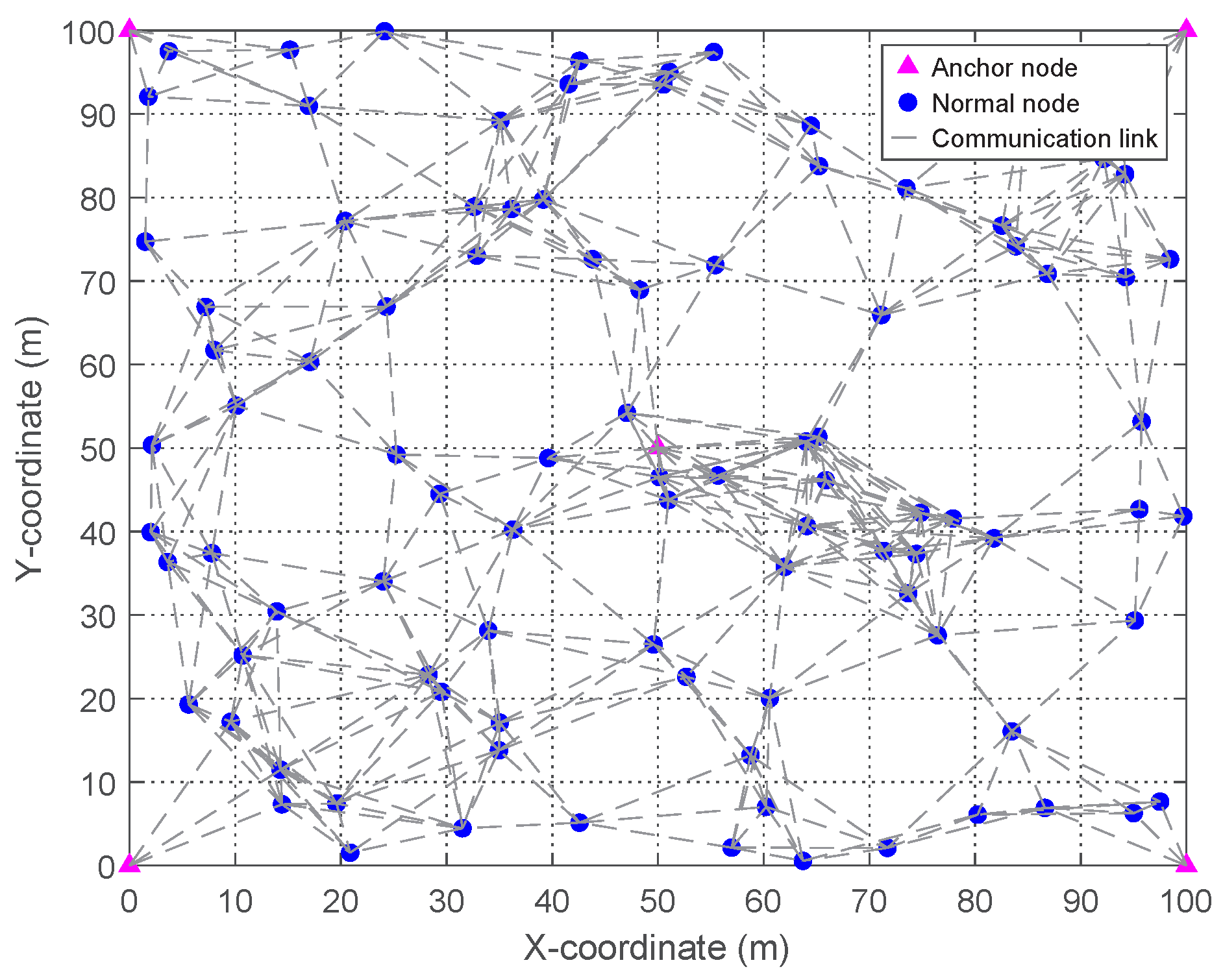
To evaluate the proposed algorithm, simulations are performed in a $100\times 100$ m² square monitoring area containing 100 sensor nodes. Among them, five anchor nodes are placed at the four corners and the center, while the remaining 95 normal nodes are randomly and uniformly distributed. The resulting network topology is illustrated in Figure 2, where dotted lines represent direct communication links within a specified radius. To emulate real-world measurement errors, Gaussian and outlier noise are added to the original distance matrix $\mathbf{D}$, yielding a corrupted version $\tilde{\mathbf{D}}$. A subset of its entries is then randomly sampled to form the observed matrix $\mathbf{S}$. The simulation parameters are listed in

Table 1. Simulation parameters.

Parameter	Symbol	Value
Area of sensing area	$Area$	$100\times 100$ m2
Number of sensor nodes	N	100
Number of anchor nodes	M	5
Gaussian noise	$G_n$	$N{\left(0,10\right)}^2$
Outlier noise	$Outlier$	$\left[5000,10,000\right]$

.

For performance evaluation, the proposed algorithm is compared with several state-of-the-art matrix completion methods, including Semidefinite Relaxation Localization (SDRL) [12], Matrix Decomposition via Truncated nuclear norm and Sparse regularizer (MDTS) [35], Matrix Completion with column Outlier and Sparse noise (MCOS) [34], and Online Robust Matrix Completion (ORMC) [31]. To assess robustness under various noise conditions, four experimental scenarios are considered: (1) noise-free, (2) Gaussian noise only, (3) outlier noise only, and (4) combined Gaussian and outlier noise. All simulations are implemented in MATLAB R2022a on a Windows 10 (64-bit) system with an Intel Core i7-7700k CPU (4.2 GHz) and 16 GB RAM. Each experiment is repeated 100 times, and the average results are reported.

To quantitatively evaluate the performance of the proposed algorithm, two error metrics are adopted and defined as follows:

• Average Completion Error (ACE):

  $$ACE=E\left\{{{∥\widehat{\mathbf{D}}-\mathbf{D}∥}_F/\phantom{{∥\widehat{\mathbf{D}}-\mathbf{D}∥}_F∥\mathbf{D}∥}∥\mathbf{D}∥}_F\right\},$$

  (28)
• Average Localization Error (ALE):

  $$ALE={∥\widehat{\mathbf{X}}-\mathbf{X}∥}_F/\phantom{{∥\widehat{X}-X∥}_{F}N}N,$$

  (29)

  where $\widehat{\mathbf{X}}$ represents the estimated coordinate matrix, and $\mathbf{X}$ denotes the true coordinate matrix of the node.

5.2. Simulation Results and Analysis

5.2.1. Noise-Free Scenario

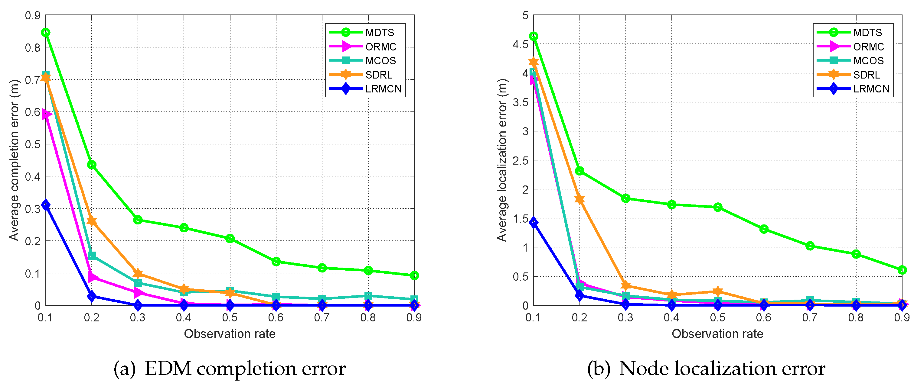
In this experiment, it is assumed that there is no noise interference during the measurement of inter-node distances; that is, the collected EDM contains missing entries but is not corrupted by any noise. Figure 3a,b present the EDM completion error and node localization error, respectively, for the five algorithms under different observation rates. The observation rate is defined as the ratio of the number of observed entries in the sampling matrix to the total number of elements in the complete EDM.

As illustrated in Figure 3, both the average EDM completion error and the node localization error for all five algorithms decrease significantly as the observation rate increases in the absence of noise. Specifically, Figure 3a shows that the proposed LRMCN consistently outperforms the other four algorithms in terms of matrix reconstruction accuracy under noise-free conditions. When the observation rate reaches 0.3, LRMCN achieves a near-zero reconstruction error, while the errors for MDTS, ORMC, MCOS, and SDRL are approximately 0.26 m, 0.04 m, 0.07 m, and 0.10 m, respectively. Furthermore, ORMC converges to a near-zero error when the observation rate exceeds 0.4, and SDRL exhibits similar behavior when the rate exceeds 0.6. In contrast, MCOS and MDTS fail to reach a zero error level across all tested observation rates.

Comparing Figure 3a and Figure 3b, the localization errors closely follow the trend of matrix completion errors. The proposed LRMCN achieves the lowest localization error across all observation rates, accurately localizing nodes even at a relatively low observation rate of 0.3 and outperforming all baseline algorithms. This is because, in MDS-based localization, a complete and accurate EDM allows the positions of all nodes to be determined from just a few anchor nodes. As shown in Figure 3a, when the observation rate exceeds 0.3, the method can effectively recover missing distances, resulting in precise node coordinates with negligible error, as illustrated in Figure 3b.

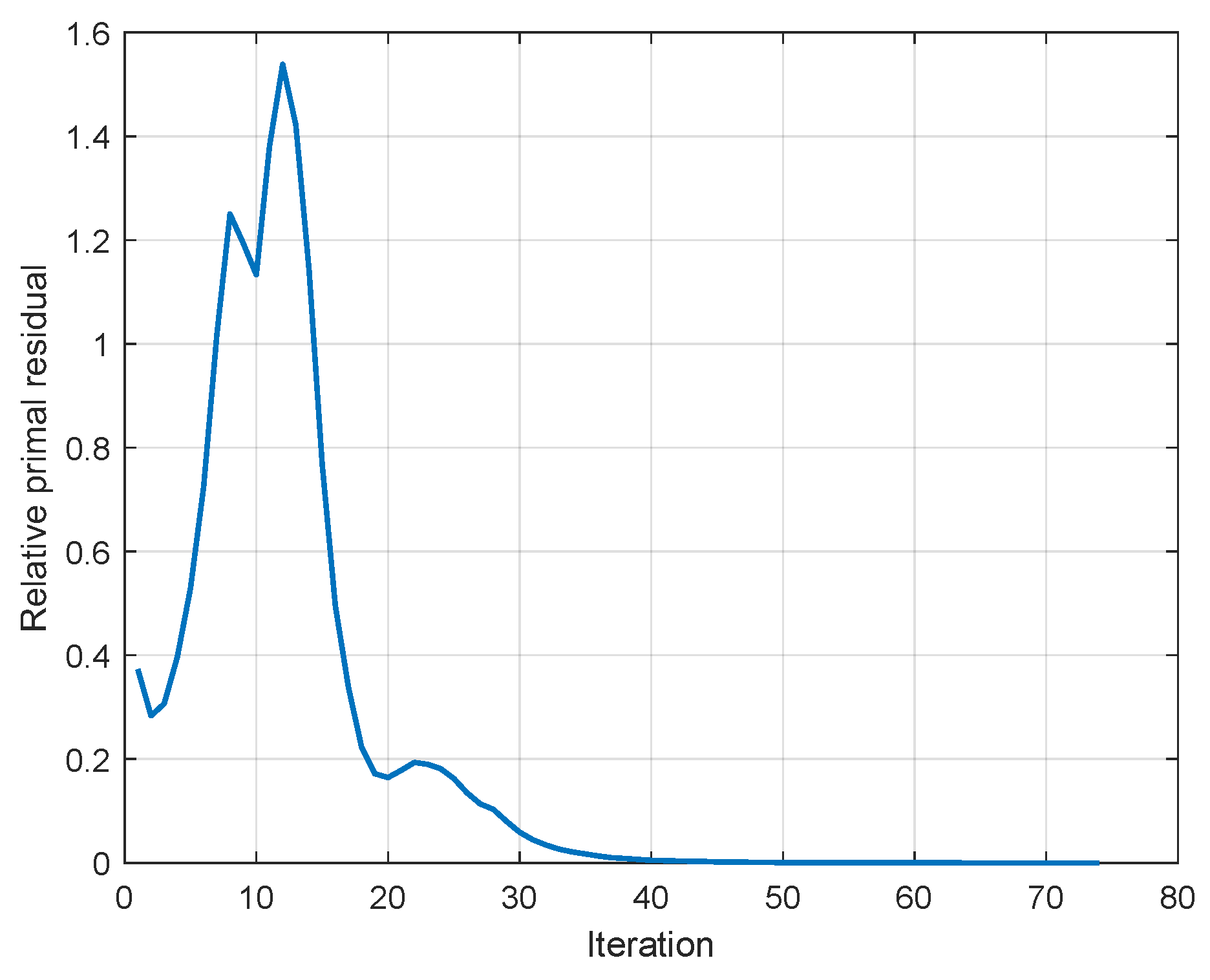
To further demonstrate the numerical convergence of the proposed nonconvex ADMMs algorithm, we plot the evolution of the relative primal residual with respect to iterations. As shown in Figure 4, slight oscillations occur in the early stage because the alternating updates of variables can temporarily increase the residual. The residual then decreases rapidly and stabilizes near zero within about 40 iterations. This behavior indicates that once the iterates enter a stable region, the updates reinforce feasibility, confirming the practical convergence and stability of our method, despite the absence of a rigorous theoretical guarantee for nonconvex objectives.

5.2.2. Gaussian Noise Scenario

In this experiment, the collected inter-node distance data is assumed to be affected solely by Gaussian noise. Specifically, zero-mean Gaussian noise with a variance of 100 is added to the distance matrix. Figure 5a,b illustrate the variation of ACE and ALE for the five algorithms under different observation rates in the presence of Gaussian noise, respectively.

As can be seen from Figure 5a, under the influence of Gaussian noise, the EDM completion errors of ORMC, SDRL, and the proposed LRMCN gradually approach zero as the observation rate increases. This indicates that these three algorithms are capable of effectively mitigating the impact of Gaussian noise in the EDM. Notably, the LRMCN achieves accurate matrix recovery when the observation rate reaches 0.3, whereas ORMC and SDRL require observation rates of 0.5 and 0.7, respectively, to achieve similar performance. In contrast, MDTS and MCOS consistently exhibit higher reconstruction errors and fail to achieve accurate EDM completion, even at high observation rates.

Figure 5b further demonstrates that LRMCN outperforms the other four algorithms in terms of node localization accuracy. Specifically, even at a low observation rate of 0.1, LRMCN achieves a node localization error of only 1.3 m. This corresponds to reductions of 65%, 62%, 70%, and 67% compared to the localization errors of MDTS, ORMC, MCOS, and SDRL, respectively. These results clearly demonstrate that the proposed LRMCN not only exhibits strong robustness to Gaussian noise but also maintains high localization accuracy under sparse observations.

5.2.3. Outlier Noise Scenario

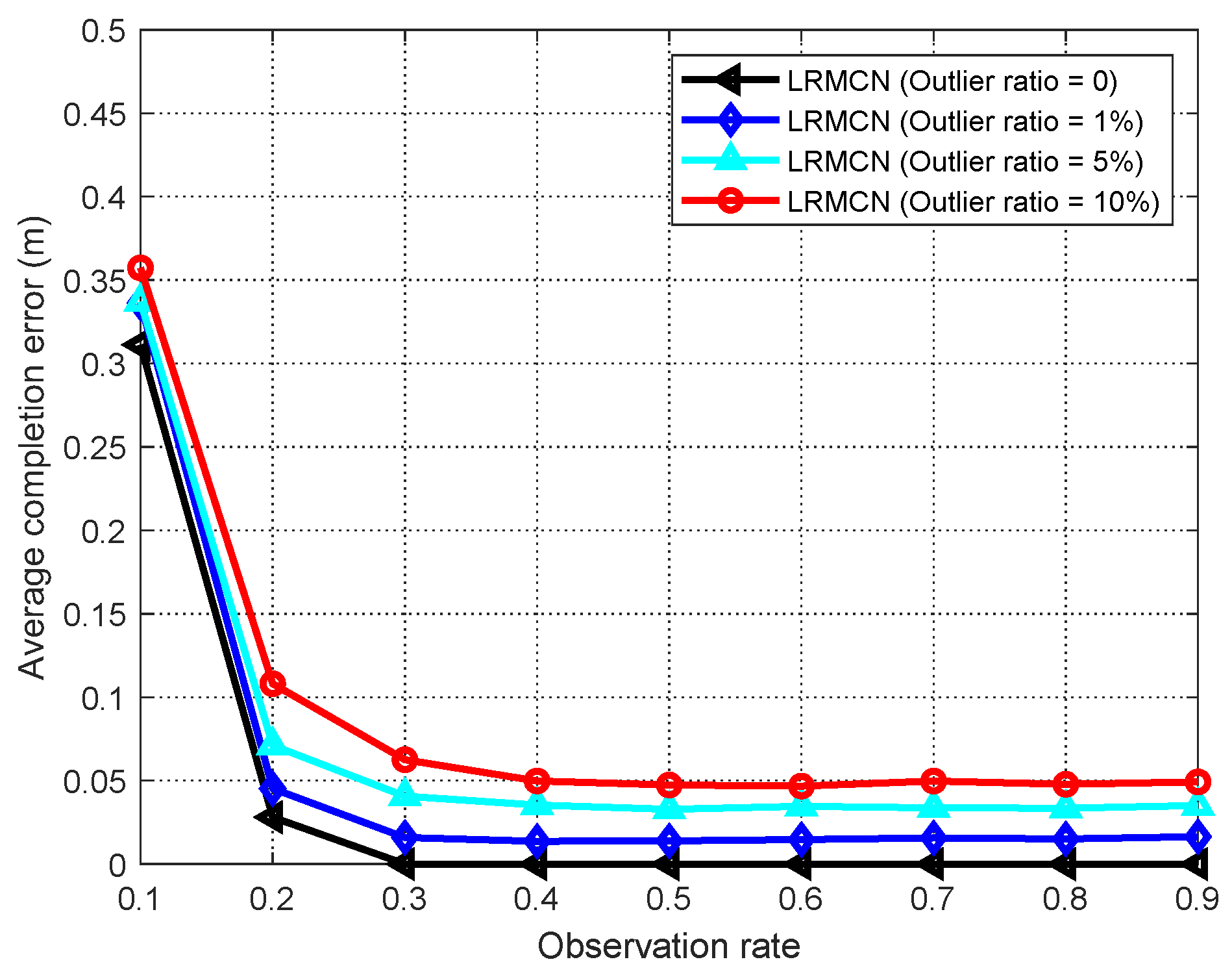
In this experiment, only outlier noise is considered. To simulate this, random values between 5000 and 10,000 are added to a subset of entries in the EDM, representing severely corrupted distance measurements. Figure 6 illustrates the performance of LRMCN under different outlier noise ratios, specifically 0, 1%, 5%, and 10%. As shown in Figure 6, the matrix completion error increases significantly with the outlier ratio, indicating that such noise severely affects the accuracy of matrix recovery. This highlights the necessity of robust noise handling in practical scenarios where large measurement deviations are likely to occur.

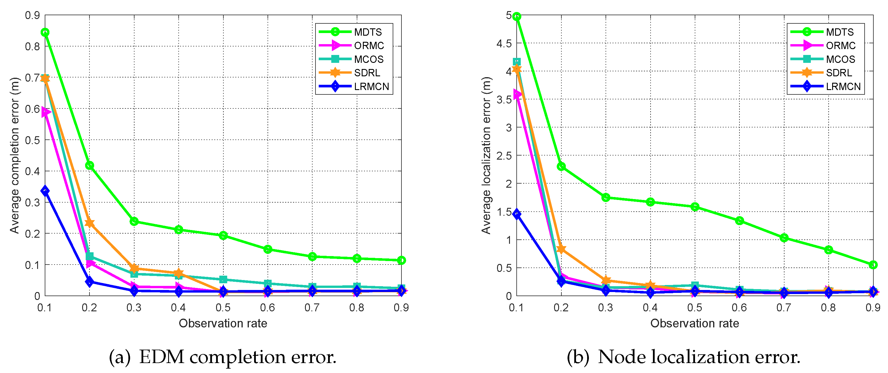
Figure 7a,b illustrate the EDM completion error and node localization error of the five algorithms under 1% outlier noise contamination. As shown in Figure 7a, LRMCN achieves the lowest completion error among all methods. Specifically, it obtains an error of 0.03 m when the observation rate reaches 0.4, while ORMC and SDRL require observation rates of at least 0.5 to achieve similar accuracy. Figure 7b further demonstrates that LRMCN also yields the lowest node localization error under the same noise conditions. These results confirm that LRMCN exhibits superior robustness against outlier noise compared to the other four benchmark algorithms.

5.2.4. Mixed Noise Scenario

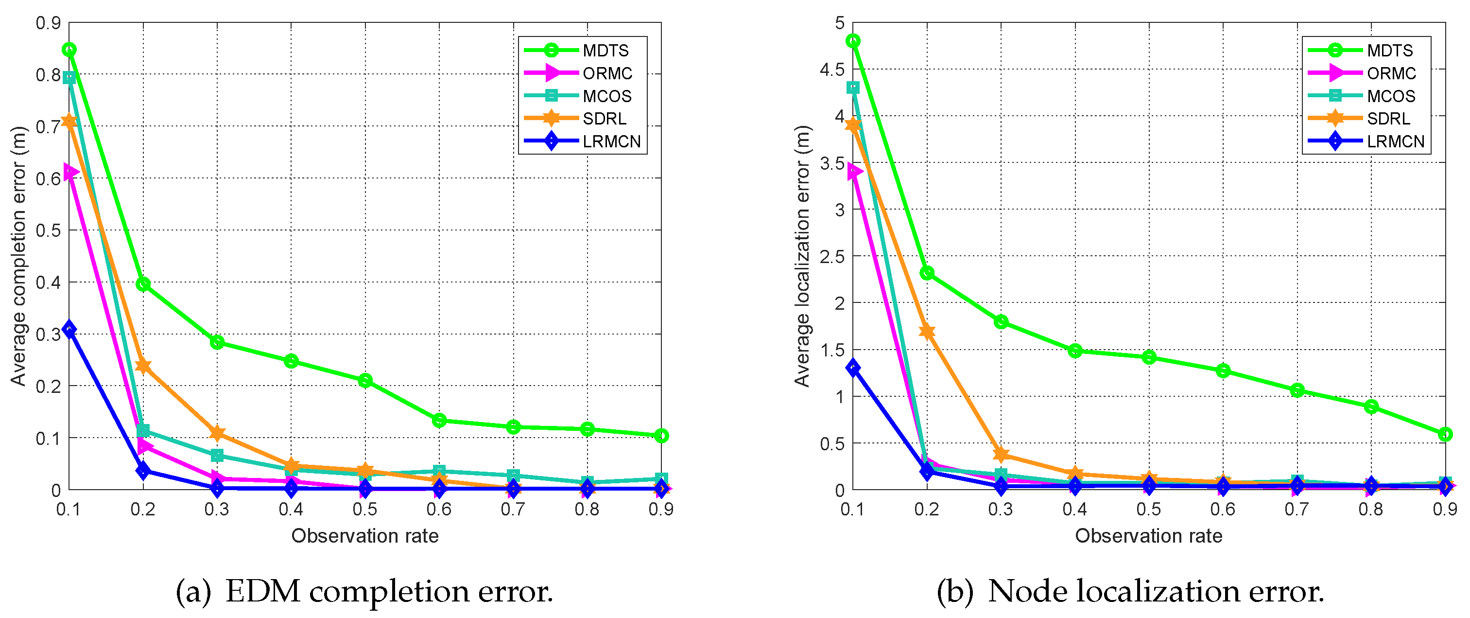
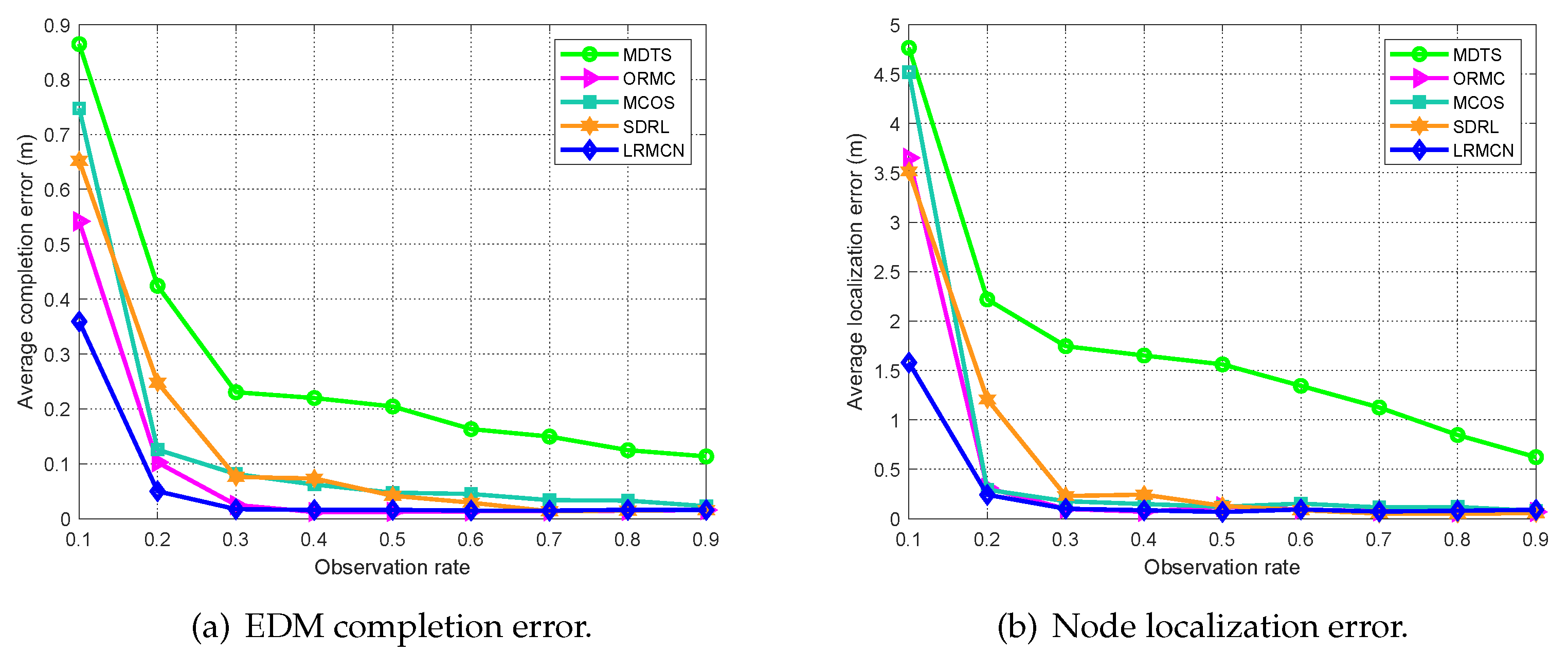
In this experiment, the inter-node distance measurements are simultaneously affected by both Gaussian and outlier noise. Specifically, Gaussian noise with a mean of 0 and a variance of 100 is added to all distance values, while outlier noise, randomly selected from the range [5000, 10,000], is injected into 1% of the matrix elements to simulate severe outlier contamination. Figure 8a,b illustrate the EDM completion error and node localization error of the five algorithms under this mixed noise scenario, respectively.

As shown in Figure 8, compared to the noise-free and single-noise scenarios, the proposed LRMCN exhibits only a slight overall increase in both matrix completion error and node localization error under mixed noise conditions. Notably, when the observation ratio exceeds 30%, both error metrics drop rapidly and stabilize, indicating that the algorithm maintains high accuracy in matrix recovery and node localization even in the presence of severe noise interference. Specifically, Figure 8a demonstrates that both LRMCN and ORMC achieve superior matrix completion performance under mixed noise, effectively suppressing Gaussian noise and mitigating the impact of outliers. When the observation rate reaches 0.3, both algorithms stabilize the completion error around 0.02 m. In contrast, SDRL and MCOS require observation rates of 0.7 and 0.9, respectively, to reach the same level of accuracy, while MDTS continues to exhibit relatively large errors even at high observation rates. Although ORMC matches the performance of LRMCN at higher observation rates (≥0.3), its accuracy degrades significantly when the observation rate falls below 0.2, highlighting the robustness of LRMCN under sparse observations.

Similarly, Figure 8b shows a consistent trend in node localization accuracy. LRMCN maintains a low localization error despite mixed noise interference and stabilizes below 0.2 m when the observation rate exceeds 30%. These results confirm that the proposed LRMCN algorithm is not only resilient to complex noise environments but also achieves high accuracy in both matrix completion and node localization tasks under limited observations. The reason is that the nonconvex $\gamma$-norm penalizes small singular values more strongly while retaining large ones, which reduces the bias of convex relaxations and preserves the dominant structural information. This property allows the proposed method to achieve more accurate recovery under low observation rates.

Table 2. Localization error reduction of baseline algorithms relative to LRMCN (observation ratio = 30%; outlier ratio = 10%).

Algorithm	Mean (m)	95% CI	p-Value	Cohen’s d
MDTS	2.296	[2.171, 2.420]	<1 $\times {10}^{-8}$	3.61
ORMC	0.152	[0.066, 0.239]	<1 $\times {10}^{-8}$	0.34
MCOS	0.037	[−0.053, 0.127]	<1 $\times {10}^{-8}$	0.08
SDRL	0.019	[−0.051, 0.089]	<1 $\times {10}^{-8}$	0.05

presents the statistical comparison between LRMCN and the four baseline algorithms over 100 independent runs. Localization errors were evaluated using the Wilcoxon signed-rank test with corresponding 95% confidence intervals. The results indicate that LRMCN consistently achieves lower localization errors than all competing methods, with p-values well below ${10}^{-8}$. The largest improvement is observed against MDTS, with a mean reduction of 2.296 m, while notable gains are also observed over ORMC, MCOS, and SDRL. In addition, the confidence intervals for all methods either exclude or are narrowly around zero, highlighting the statistical robustness of the differences. These results demonstrate that LRMCN not only attains superior localization accuracy but also provides stable and meaningful improvements in challenging, noisy, and low-observation scenarios.

5.3. Performance Evaluation Under Different Network Scales

To further evaluate the effectiveness of the proposed LRMCN algorithm, we conducted experiments on networks of varying scales.

Table 3. Performance comparison of five algorithms under different network scales (observation ratio = 30%; outlier ratio = 10%).

BEDM Size	Algorithm	Matrix Reconstruction Error	Node Localization Error	Runtime (s)
$100\times 100$	MDTS	0.8373	2.4998	0.4898
	ORMC	0.1334	0.4252	0.0367
	MCOS	0.2288	0.6999	0.0782
	SDRL	0.1313	1.2799	18.6413
	LRMCN	0.1084	0.4047	0.0101
$200\times 200$	MDTS	0.8448	1.5258	1.4797
	ORMC	0.1031	0.2168	0.0383
	MCOS	0.1473	0.2181	0.2387
	SDRL	0.1423	0.3151	247.2405
	LRMCN	0.1001	0.1434	0.0335
$300\times 300$	MDTS	0.8489	0.9839	3.8228
	ORMC	0.1005	0.1221	0.0608
	MCOS	0.1354	0.1382	0.4187
	SDRL	0.1305	0.1988	1.46 × 103
	LRMCN	0.0959	0.0961	0.0467

reports the matrix completion error, localization error, and running time of five algorithms under different network scales with an observation rate of 30% and an outlier noise ratio of 10%. The results indicate that as the network size increases, the completion accuracy of all algorithms improves, leading to more accurate node localization. This improvement can be attributed to the fact that larger distance matrices exhibit stronger low-rank properties, thereby enhancing the effectiveness of matrix completion.

Among the five algorithms, the proposed LRMCN consistently achieves the lowest EDM completion error and localization error across all network scales while also requiring the least running time. For example, when the network size is $N=300$, LRMCN achieves excellent completion and localization performance using only $30\%$ of the observed data, with a runtime of just 0.0467 s. This runtime is substantially faster than that of MDTS by $98.3\%$, ORMC by $23.2\%$, and MCOS by $88.9\%$. In contrast, SDRL incurs substantial computational overhead due to repeated singular-value decompositions, making it unsuitable for large-scale WSNs. These results demonstrate that LRMCN not only ensures superior accuracy but also reduces communication overhead, thereby lowering energy consumption and extending the network lifetime.

5.4. Visualization of Localization Result

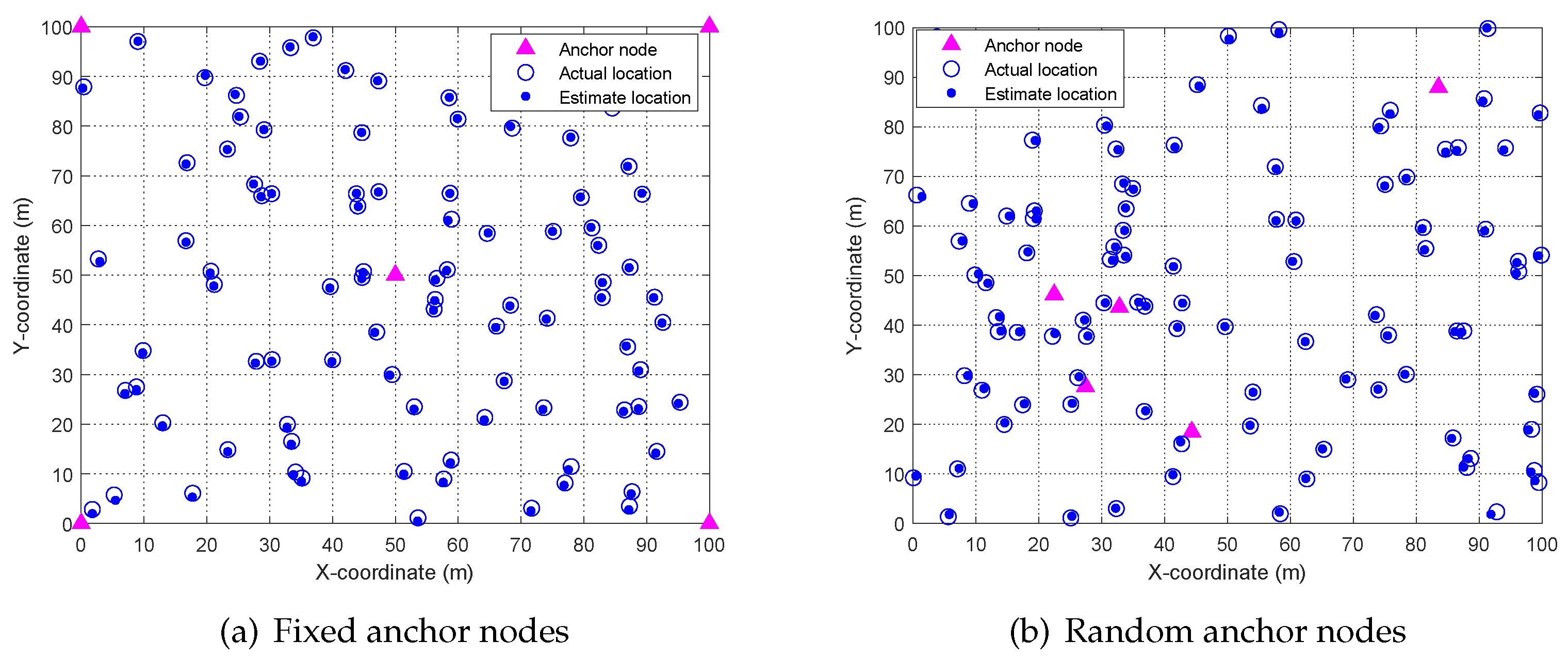
Figure 9 illustrates the final localization results of 100 sensor nodes under two different anchor settings. In Figure 9a, anchor nodes are placed at predetermined positions, where solid triangles indicate the true anchor locations, hollow circles represent the actual positions of regular sensor nodes, and solid dots denote their estimated positions obtained using the proposed LRMCN-based localization algorithm. In Figure 9b, the anchor nodes are randomly placed, while the other experimental parameters remain the same, with an observation rate of 30%, Gaussian noise, and $1\%$ outlier noise. In both cases, most estimated positions (solid dots) are closely aligned with the actual positions (hollow circles), demonstrating that the proposed algorithm can achieve accurate localization even under partial distance measurements, mixed noise interference, and varying anchor deployments.

6. Conclusions and Future Work

To address the challenges of incomplete and noise-contaminated EDMs in WSNs, a node localization algorithm based on matrix decomposition is proposed. The method leverages the low-rank property of the EDM by factorizing the sampled distance matrix into two low-dimensional submatrices, which imposes structural constraints and reduces computational complexity. A nonconvex surrogate function is introduced to approximate the matrix rank, and the optimization problem is solved using the ADMMs, enabling accurate recovery of the full EDM from sparse and noisy data. After matrix completion, relative node positions are estimated using classical multi-dimensional scaling, and absolute coordinates are obtained with the aid of a few anchor nodes. Experimental results under various noise conditions demonstrate that the algorithm achieves high localization accuracy using limited distance information. It also exhibits strong robustness to both Gaussian and outlier noise, supporting applications such as fault detection, task scheduling, and routing optimization in large-scale networks. Future work will further extend our approach by exploring comparisons and integrations with deep learning methods such as GNNs and autoencoders.

References

1. Wang, R.; Xu, C.; Sun, J.; Duan, S.; Zhang, X. Cooperative Localization for Multi-Agents Based on Reinforcement Learning Compensated Filter. IEEE J. Sel. Areas Commun. 2024, 42, 2820–2831. [Google Scholar] [CrossRef]
2. Tu, Q.; Liu, X.; Xie, Y.; Han, G. Range-Free Localization Using Extreme Learning Machine and Ring-Shaped Salp Swarm Algorithm in Anisotropic Networks. IEEE Internet Things J. 2023, 10, 8228–8244. [Google Scholar] [CrossRef]
3. Kim, S.; Nguyen, L.T.; Kim, J.; Shim, B. Deep Learning Based Low-Rank Matrix Completion for IoT Network Localization. IEEE Wirel. Commun. Lett. 2021, 10, 2115–2119. [Google Scholar] [CrossRef]
4. Zhu, L.; Mu, J.; Yu, L.; Liu, Y.; Zhu, F.; Gu, J. Federated Learning-Based Location Similarity Model for Location Privacy Preserving Recommendation. Electronics 2025, 14, 2578. [Google Scholar] [CrossRef]
5. Sorbelli, F.B.; Pinotti, C.M.; Silvestri, S.; Das, S.K. Measurement Errors in Range-Based Localization Algorithms for UAVs: Analysis and Experimentation. IEEE Trans. Mob. Comput. 2022, 21, 1291–1304. [Google Scholar] [CrossRef]
6. Jiang, P.; Gu, X.; Zhou, H. Cooperative Positioning of Wireless Networks in Complex Propagation Environments. IEEE J. Sel. Areas Commun. 2024, 42, 2877–2889. [Google Scholar] [CrossRef]
7. Qin, S.; Xiaowei, C.; Sihao, Z.; Shuang, X.; Mingquan, L. BLAS: Broadcast Relative Localization and Clock Synchronization for Dynamic Dense Multi-Agent Systems. IEEE Trans. Aerosp. Electron. Syst. 2020, 56, 3822–3839. [Google Scholar]
8. Guo, X.; Chu, L.; Sun, X. Accurate Localization of Multiple Sources Using Semidefinite Programming Based on Incomplete Range Matrix. IEEE Sens. J. 2016, 16, 5319–5324. [Google Scholar] [CrossRef]
9. Tian, C.; Ma, Y.; Liang, X.; Ning, W.; Zhao, H. On Absoluteness and Stationary Condition of WMDS for Range-Based Localization. IEEE Internet Things J. 2023, 10, 10066–10079. [Google Scholar] [CrossRef]
10. Khattak, S.B.A.; Jia, M.; Marey, M.; Nasralla, M.M.; Guo, Q.; Gu, X. A novel single anchor localization method for wireless sensors in 5G satellite-terrestrial network. Alex. Eng. J. 2022, 61, 5595–5606. [Google Scholar] [CrossRef]
11. Bouchoucha, T.; Chuah, C.N.; Ding, Z. Topology inference of unknown networks based on robust virtual coordinate systems. IEEE/ACM Trans. Netw. 2019, 27, 405–418. [Google Scholar] [CrossRef]
12. Guo, X.; Chu, L.; Ansari, N. Joint localization of multiple sources from incomplete noisy Euclidean distance matrix in wireless networks. Comput. Commun. 2018, 122, 20–29. [Google Scholar] [CrossRef]
13. Xiao, F.; Liu, W.; Li, Z.; Chen, L.; Wang, R. Noise-tolerant wireless sensor networks localization via multinorms regularized matrix completion. IEEE Trans. Veh. Technol. 2017, 67, 2409–2419. [Google Scholar] [CrossRef]
14. Xiao, F.; Chen, L.; Sha, C.; Sun, L.; Wang, R.; Liu, A.X.; Ahmed, F. Noise tolerant localization for sensor networks. IEEE/ACM Trans. Netw. 2018, 26, 1701–1714. [Google Scholar] [CrossRef]
15. Gao, K.; Huang, Z.H.; Guo, L. Low-rank matrix recovery problem minimizing a new ratio of two norms approximating the rank function then using an ADMM-type solver with applications. J. Comput. Appl. Math. 2024, 438, 115564. [Google Scholar] [CrossRef]
16. Jiang, P.; Zhuang, Z.; Xie, W. Gram Matrix Completion for Cooperative Localization in Partially Connected Wireless Sensor Network. IEEE Signal Process. Lett. 2024, 31, 939–943. [Google Scholar] [CrossRef]
17. Al-Homidan, S.; Wolkowicz, H. Approximate and exact completion problems for Euclidean distance matrices using semidefinite programming. Linear Algebra Its Appl. 2005, 406, 109–141. [Google Scholar] [CrossRef]
18. Cai, J.F.; Candès, E.J.; Shen, Z. A singular value thresholding algorithm for matrix completion. SIAM J. Optim. 2010, 20, 1956–1982. [Google Scholar] [CrossRef]
19. Lin, Z.; Ganesh, A.; Wright, J.; Wu, L.; Chen, M.; Ma, Y. Fast Convex Optimization Algorithms for Exact Recovery of a Corrupted Low-Rank Matrix; Report no. UILU-ENG-09-2214, DC-246; Coordinated Science Laboratory, University of Illinois: Champaign, IL, USA, 2009. [Google Scholar]
20. Toh, K.C.; Yun, S. An accelerated proximal gradient algorithm for nuclear norm regularized linear least squares problems. Pac. J. Optim. 2010, 6, 15. [Google Scholar]
21. Candès, E.J.; Tao, T. The power of convex relaxation: Near-optimal matrix completion. IEEE Trans. Inf. Theory 2010, 56, 2053–2080. [Google Scholar] [CrossRef]
22. Saeedi, T.; Rezghi, M. A novel enriched version of truncated nuclear norm regularization for matrix completion of inexact observed data. IEEE Trans. Knowl. Data Eng. 2020, 34, 519–530. [Google Scholar] [CrossRef]
23. Liang, H.; Kang, L.; Huang, J. A robust low-rank matrix completion based on truncated nuclear norm and Lp-norm. J. Supercomput. 2022, 78, 12950–12972. [Google Scholar] [CrossRef]
24. Lu, C.; Tang, J.; Yan, S.; Lin, Z. Nonconvex nonsmooth low rank minimization via iteratively reweighted nuclear norm. IEEE Trans. Image Process. 2015, 25, 829–839. [Google Scholar] [CrossRef]
25. Li, X.; Zhu, Z.; Man-Cho So, A.; Vidal, R. Nonconvex robust low-rank matrix recovery. SIAM J. Optim. 2020, 30, 660–686. [Google Scholar] [CrossRef]
26. Chen, L.; Jiang, X.; Liu, X.; Zhou, Z. Logarithmic norm regularized low-rank factorization for matrix and tensor completion. IEEE Trans. Image Process. 2021, 30, 3434–3449. [Google Scholar] [CrossRef]
27. Huang, M.; Ma, S.; Lai, L. Robust Low-Rank Matrix Completion via an Alternating Manifold Proximal Gradient Continuation Method. IEEE Trans. Signal Process. 2021, 69, 2639–2652. [Google Scholar] [CrossRef]
28. Nguyen, L.T.; Kim, J.; Kim, S.; Shim, B. Localization of IoT Networks via Low-Rank Matrix Completion. IEEE Trans. Commun. 2019, 67, 5833–5847. [Google Scholar] [CrossRef]
29. Zhang, H.; Liu, Y.; Lei, H. Localization from incomplete euclidean distance matrix: Performance analysis for the svd–mds approach. IEEE Trans. Signal Process. 2019, 67, 2196–2209. [Google Scholar] [CrossRef]
30. Giampouras, P.V.; Rontogiannis, A.A.; Koutroumbas, K.D. Alternating iteratively reweighted least squares minimization for low-rank matrix factorization. IEEE Trans. Signal Process. 2018, 67, 490–503. [Google Scholar] [CrossRef]
31. Nie, F.; Li, Z.; Hu, Z.; Wang, R.; Li, X. Robust matrix completion with column outliers. IEEE Trans. Cybern. 2021, 52, 12042–12055. [Google Scholar] [CrossRef]
32. Wang, S.; Wang, Y.; Chen, Y.; Pan, P.; Sun, Z.; He, G. Robust PCA using matrix factorization for background/foreground separation. IEEE Access 2018, 6, 18945–18953. [Google Scholar] [CrossRef]
33. Zhang, L.; Peng, L.; Zhang, T.; Cao, S.; Peng, Z. Infrared small target detection via non-convex rank approximation minimization joint l 2, 1 norm. Remote Sens. 2018, 10, 1821. [Google Scholar] [CrossRef]
34. Li, Z.; Hu, Z.; Nie, F.; Wang, R.; Li, X. Matrix completion with column outliers and sparse noise. Inf. Sci. 2021, 573, 125–140. [Google Scholar] [CrossRef]
35. Xue, Z.; Dong, J.; Zhao, Y.; Liu, C.; Chellali, R. Low-rank and sparse matrix decomposition via the truncated nuclear norm and a sparse regularizer. Vis. Comput. 2019, 35, 1549–1566. [Google Scholar] [CrossRef]
Figure 1. Rank function approximations of different norms.
Electronics 14 03920 g001
Figure 2. Network topology.
Electronics 14 03920 g002
Figure 3. Performance comparison of different algorithms without noise.
Electronics 14 03920 g003
Figure 4. Convergence curve of the proposed nonconvex ADMMs algorithm.
Electronics 14 03920 g004
Figure 5. Performance comparison of different algorithms with Gaussian noise.
Electronics 14 03920 g005
Figure 6. Matrix completion error of LRMCN with different outlier noise ratios.
Electronics 14 03920 g006
Figure 7. Performance comparison of different algorithms with outlier noise (outlier ratio = 1 % ).
Electronics 14 03920 g007
Figure 8. Performance comparison of different algorithms with mixed noise (outlier ratio = 1 % ).
Electronics 14 03920 g008
Figure 9. Localization results under different anchor deployments (observation ratio = 30%; outlier ratio = 1%).
Electronics 14 03920 g009