1. Introduction
The rapidly increasing demand for wireless transmission of high-resolution three-dimensional (3D) image and video signals poses a significant challenge to current communication systems [
1]. Emerging applications such as the metaverse, augmented/virtual reality (AR/VR), remote surgery, and vehicular-to-everything (V2X) require robust transmission and realistic reconstruction of 3D data in fast-varying wireless environments with limited bandwidth resources [
2,
3,
4,
5]. State-of-the-art (SOTA) digital communication systems are designed based on Shannon’s source–channel separation theorem, which is optimal only under asymptotic and idealized assumptions [
6]. In practical scenarios with finite block-lengths and non-ergodic channel statistics, these separation-based systems are suboptimal [
7,
8] and suffer from the “cliff effect”—a sudden drop in quality when the channel signal-to-noise ratio (SNR) falls below a specific threshold [
9].
Joint source–channel coding (JSCC) has long been studied as a powerful alternative to improve end-to-end performance in practical systems [
10,
11]. Rather than separating source and channel coding, JSCC schemes create a direct mapping from the source data to the channel input symbols. More recently, in the context of semantic communications [
12], deep learning-based JSCC (DeepJSCC) methods have shown remarkable results [
13,
14,
15]. By learning the end-to-end mapping from data, these methods exhibit strong resilience to channel variations and provide graceful performance degradation, making them ideal for unreliable wireless channels [
16,
17,
18,
19,
20].
While JSCC provides a powerful framework for how to transmit data robustly, a critical and complementary question is what data to transmit to maximize efficiency, especially for high-dimensional sources like 3D images. Transmitting raw 3D point clouds or dense meshes is often prohibitively expensive in terms of bandwidth. A more semantic approach is to extract and transmit only the most salient geometric features that define the object’s shape. In nature, shapes are often characterized by common features like curves that define bending and direction [
21]. Features which are extracted by well-chosen 3D curves can provide a much richer and more compact geometrical description than a sparse set of 3D landmarks [
22].
Significant research has been dedicated to estimating such characteristic curves from 3D data. These methods can be grouped into two categories: estimation from point clouds and from triangulated meshes. For point clouds, techniques like Robust Moving Least Squares (RMLS) have been used to identify points of high curvature, which are then connected to form feature curves [
21,
23]. Ridges and valleys detected on meshes are powerful features for describing shape [
24,
25,
26]. Others have used principal curvatures to select and smooth feature lines [
27]. However, a common challenge with these methods is ensuring the connectivity of the estimated curves, which is crucial for reconstructing a coherent shape [
25,
27,
28].
More recently, machine learning and deep learning have provided effective methods for feature extraction. Deep Neural Networks (DNNs) have been used to extract object contours, and 3D leaf reconstruction methods have integrated 2D image segmentation with 3D curve techniques [
29]. These methods, while powerful, often require massive training datasets to achieve high accuracy and can be computationally intensive [
30]. The field of mesh segmentation also offers relevant techniques for partitioning a mesh into meaningful parts, although often without focusing on the smoothness of the partition boundaries [
31,
32,
33,
34,
35]. Specialized tools like FiberMesh have also been developed to manipulate mesh structures along user-defined paths. The work in [
36] proposed a DNN-based indoor localization framework that leverages generative adversarial networks (GANs) and semi-supervised learning to mitigate the issue of limited datasets, demonstrating that deep neural architectures can effectively extract features and improve robustness even in data-scarce environments. This line of research highlights that data-driven techniques can complement optimization-based frameworks in wireless communications.
In this paper, we propose a novel framework for efficient and robust 3D image transmission that synergistically combines semantic 3D feature extraction with deep JSCC. Our approach deviates from transmitting the entire, dense 3D object. Instead, we first employ a lightweight algorithm to identify and extract salient geometric features—specifically, the ridge and valley curves that constitute the structural skeleton of the object. A formal mathematical analysis of the algorithm’s performance is challenging due to the complex and stochastic nature of the target images, which often include random noise and discontinuities along the curves. Therefore, this study focuses on empirically validating the method’s robustness and flexibility through simulations on these challenging cases, for which theoretical models are often insufficient.
This compact feature representation, which captures the essential geometric information, is then encoded and transmitted over the wireless channel using a purpose-built DeepJSCC scheme. By transmitting only the critical semantic features, our method dramatically reduces the required bandwidth while leveraging the robustness of JSCC to ensure high-quality reconstruction even under poor channel conditions.
To be clear, our proposed framework comprises two distinct and sequential stages: feature extraction and transmission. The scope of the zero-shot estimation is confined to the first stage, where a lightweight computational geometry algorithm acts as a semantic source encoder. It processes the dense 3D surface to extract a compact set of feature curves, operating without any prior training on specific object classes. The scope of the DeepJSCC scheme covers the second stage, where it takes these extracted features as input and learns a robust mapping to channel symbols for transmission. In summary, the zero-shot method determines what critical information to send, while the trained DeepJSCC module determines how to send it resiliently.
The contributions of this paper are outlined as follows.
Introduction of a novel zero-shot 3D estimation method which directly works on 3D surfaces with limited numbers of landmarks.
Illustration of the flexibility which works on complex surfaces with noises nearby.
Higher quality for the same cost. With identical bandwidth and power, the hybrid method produces a better-quality reconstructed 3D image.
Graceful adaptation to channel quality. As the channel connection improves (higher SNR), the hybrid method’s performance smoothly increases, delivering an even better image. In contrast, the standard digital method’s quality is "locked in” by its fixed compression rate and does not benefit from a better connection.
The rest of this paper is organized as follows.
Section 2 provides background fundamentals used in this research. A novel approach for estimating curves on folded shapes where very few landmarks are available is presented in
Section 3.
Section 4 presents the hybrid joint source–channel coding scheme. Finally,
Section 5 is the conclusion and the future research plan.
2. Data and Basic Concepts
This research utilizes 3D images of real-world objects which are captured using the Artec
® camera system (Artec 3D, Luxembourg City, Luxembourg), such as the one shown in
Figure 1a. A 3D image is constructed by: a point cloud consisting of ordered 3D points captured by stereo cameras, as shown in
Figure 1b; a Delaunay triangulation whose triangles are consistently ordered, using the 3D points as their vertices, as shown in
Figure 1c. Thus, A 3D shape (model) produced by the camera system is characterized as a triangulated surface in this paper [
37].
Traditional local feature descriptors which define correspondences across individuals include landmarks and ridge or valley curves. The function of landmarks is to signify clearly defined corresponding locations on multiple objects [
39]. Ridge or valley curves will be referred to as “curves” throughout this paper. Three-dimensional curves are effectively described by an ordered collection of consecutive 3D coordinates situated on the object’s surface. The arc length between any two points on a 3D curve is estimated by the sum of Euclidean distances of the intermediate adjacent points. Whether they are directly measured triangle vertices or calculated intermediate locations on the facets, both landmarks and points constituting a curve are treated as residing on the surface itself.
Ridge and valley curves are characterized by their principal curvatures [
26]. (Note that our definition differs from the reference, as our surface normal vector points outwards, whereas theirs points inwards.) The maximal and minimal principal curvatures, denoted
and
, respectively (with
), measure the degree of bending along and across these curves. The principal curvatures of a point are estimated as follows. A local coordinate system can be constructed by the normal vector, an edge nearby and the cross product of them. Any vertex in the local area can be projected to the system. The projected coordinates can be fitted by a cubic polynomial of the three dimensions. The Weingarten matrix of the model provides its eigenvalues which we use as the principal curvatures and eigenvectors which are the principal vectors.
The first derivatives of the principal curvatures along these directions are defined as and , where and are the corresponding principal directions.
A curve is identified as a ridge if it satisfies:
Conversely, a curve is identified as a valley if it meets the conditions:
Physically, the negative curvature
describes the bending across a ridge, and the positive curvature
describes the bending across a valley. A larger absolute value for a principal curvature indicates a more pronounced convex or concave geometry. For convenience in this paper, we will also use the notation
and
for the first and second principal curvatures, where
.
The Shape Index (SI) is a dimensionless measure that characterizes the local shape of a surface at any given point
p [
40]. Unlike principal curvatures, which measure the magnitude of bending, the SI provides a qualitative description of the surface’s topology. The index is defined by the formula:
This formula maps the relationship between the maximal (
) and minimal (
) principal curvatures onto a fixed interval of [−1, 1]. This mapping facilitates the identification of local geometries; for example, the curve formed by closed lips is a convex feature, which corresponds to an SI value near 1. Other fundamental shapes like cups (concave) and saddles are represented by SI values of −1 and 0, respectively.
3. Curve Estimation Methodology
As established in
Section 2, a 3D curve can be represented by a sequence of discrete points. Since a 3D camera system provides an estimated manifold of the true object, any curve identified on this image is likewise an approximation of the true curve on the object’s surface. A curve can be parameterized by its arc length
s, such that a point on the curve is given by
[
41]. A key statistical principle, highlighted by Vittert, is that the estimated curve converges to the true curve as the error in the image manifold decreases.
Identifying these curves often relies on landmarks to guide their composition. However, in practice, only a sparse set of landmarks is typically available, as manually adding more is a labor-intensive and time-consuming process. This section, therefore, introduces a novel computational geometry method designed to effectively estimate 3D curves even from limited guiding data.
3.1. Methodology
At any point on a 3D surface, two orthogonal principal directions exist which correspond to the maximum and minimum surface bending (curvature). As detailed in
Section 2, for a ridge, the first principal curvature,
, aligns with the tangent along the ridge, while the second,
, is orthogonal to it. Surface creases are formally defined as “The loci of points where the largest in absolute value principal curvature takes a positive maximum (negative minimum) along its corresponding curvature line" [
26].
Drawing inspiration from this definition, our novel method identifies the loci of points forming a curve. We use the principal curvature whose direction is transverse to the curve to locate a point where this curvature reaches a local maximum in absolute value. The other principal curvature is then utilized to step to an adjacent location, positioning the search near the next point on the curve.
3.1.1. Algorithm in Detail
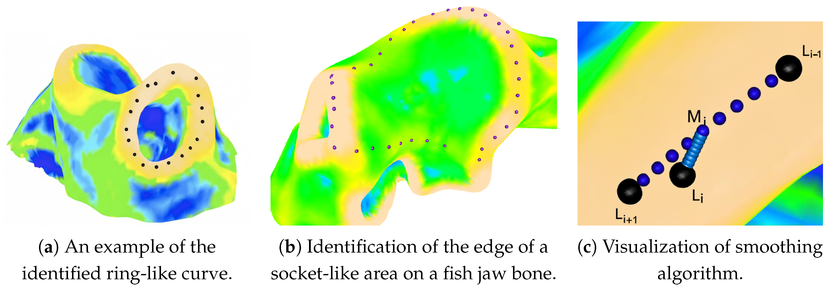
To illustrate the algorithm, we consider the identification of a ring-like ridge on the shape shown in
Figure 2 (left). The surface is colored according to the second principal curvature,
, where yellow indicates a stronger bend across the ridge. The guiding principle for identifying a ridge is to trace a path that follows the ridge’s direction and is composed of points with the maximum
bending size (For a ridge, the second principal curvature (
) is negative, so we define the
bending size as its absolute value,
.) across the ridge. These identified points form an initial approximation of the curve, which is subsequently smoothed using local neighbors.
As shown by the black point in the left panel of
Figure 2, the process is initiated from a seed. The most efficient way to place a seed is through manual placement using the IDAV Landmark Editor software v3.6 (This software is no longer available for download. An alternative is the Stratovan Checkpoint.). This system has an interface that visualizes a 3D image and provides the coordinates of a point when it is clicked. Alternatively, especially when dealing with a large number of images, the seed can also be found automatically based on its geometric characteristics, such as maximum or minimum curvature. The iterative procedure is as follows:
Beginning at a starting point (initially the seed), take a single step along the first principal direction of the surface.
From the endpoint of this step, locate the nearest vertex on the surface. At this vertex, generate a two-sided search path along its second principal direction.
Along this search path, identify the point with the maximum curvature value . This point becomes a new point on the curve and serves as the starting point for the next iteration.
Repeat steps 1–3 until a termination condition is met. For a ring-like curve, this could be returning sufficiently close to the original landmark; alternatively, it could be reaching a predefined total arc length.
Figure 2 provides a visualization of the algorithm [
37]. Let the initial landmark or seed be denoted by
. The first step, termed a
movement, involves selecting a candidate point
. This is achieved by advancing a set distance from
along its first principal direction, as illustrated by the blue line. The path is sampled by a “plane cut” which generates the set of blue points [
41]. The length of the step can be two or three times of the triangles’ edges. Since “plane cut” methods can only generate paths which cross at least one triangle further, the length of the step cannot be smaller than any edge of a triangle on the image.
Next, to locate the point of maximum local bending near , a second procedure called a comparison is performed. A two-sided “plane cut” (the red dots) is generated along the second principal direction of , indicated by the red line. The point with the highest bending size, , along this red path is identified. The nearest vertex on the mesh to this point is then selected as the next point on the curve, . This new point, , subsequently serves as the starting point for finding .
An important adjustment is made to minimize estimation error. As noted in
Section 2, only the vertices of the mesh are direct observations from the camera system. Since the “plane cut” procedure can generate points that are not vertices, we enforce a rule to maintain fidelity to the original data. Instead of directly using the point with the maximum
from the red “plane cut”, we always select its closest vertex on the triangulation. As shown in the central panel of
Figure 2, this ensures that all identified points on the curve (
) are vertices of the original mesh.
3.1.2. Direction Control
To prevent the identified curve from deviating erratically, a direction–control mechanism is implemented in each iteration. This involves creating a pair of planar “boundaries” by rotating the vector formed by the last two identified points around the normal vector of the current point. These boundaries constrain the search for the next point. For instance, in the second iteration shown in
Figure 2, the vector
is rotated around the normal at
to form two new vectors (the black lines). For this anticlockwise ring identification, rotations of
anticlockwise and
clockwise proved most effective. The two planes spanned by these rotated vectors and the normal vector at
serve as the “boundaries”. Any points on the red “plane cut” that are outside these boundaries are discarded, ensuring the search stays aligned with the direction of
.
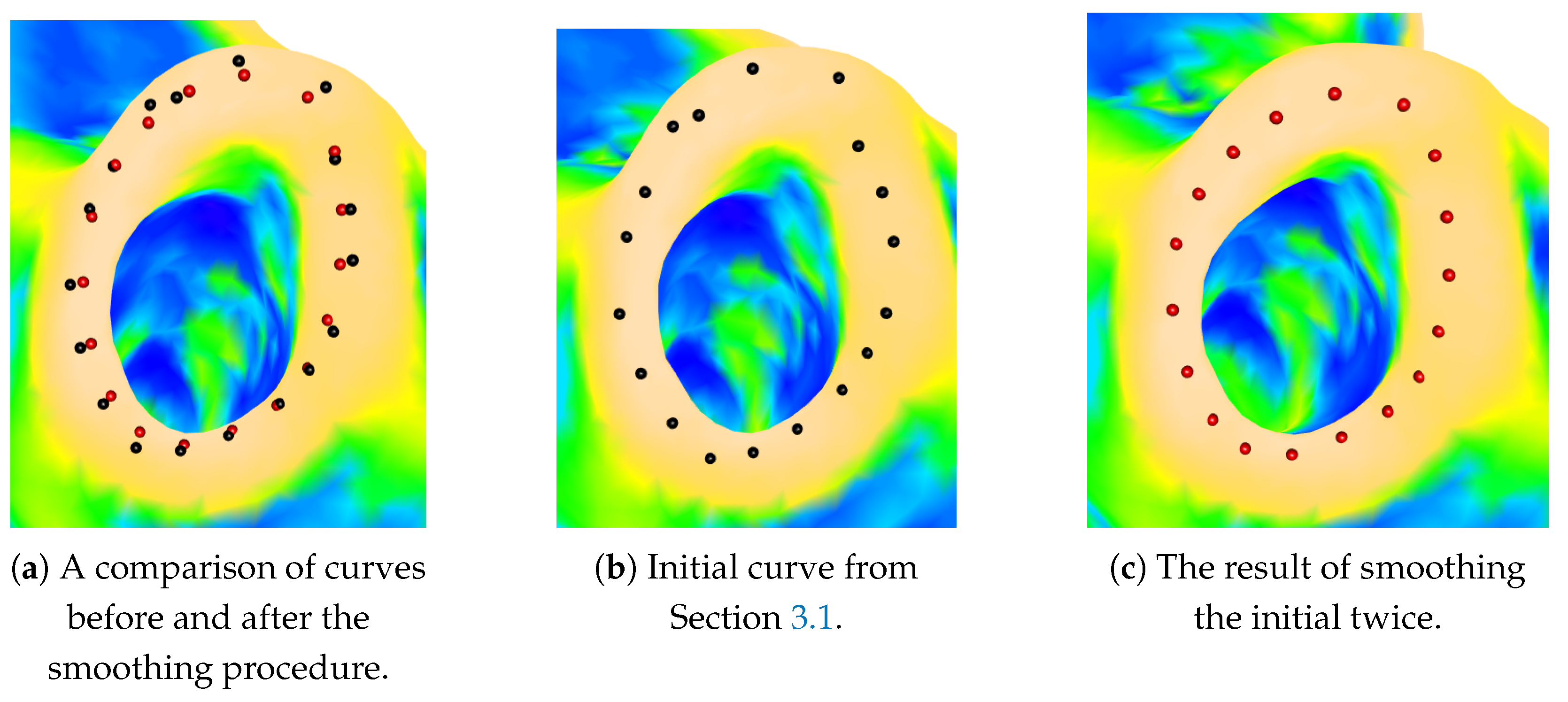
The result of this process, an “initial” curve composed of discrete points in anticlockwise order, is shown in
Figure 3a. For this example, the “movement” distance was set to 10 units per iteration, and the “comparison” search extended five units on each side of the candidate point (
). This initial curve serves as input for a subsequent smoothing procedure.
It is important to note that this method is not limited to one shape.
Figure 3b demonstrates its application in identifying the edge of a socket-like feature. Although the final curve is a closed circuit, it was generated by identifying each half independently, starting and ending at two fixed anatomical landmarks that were required to be part of the final curve.
3.1.3. Smoothing Procedure
The smoothing procedure is designed to generate a new curve with reduced variability from the initial curve. This is accomplished by calculating a new, adjusted position for each point on the initial curve.
The core principle, illustrated in
Figure 3c [
37], is to reposition each point
based on its neighbors,
and
. First, a “plane cut” representing the shortest path between
and
is created (shown as red dots). The midpoint of this path,
, can be considered the average position of the two neighbors. To incorporate the original position of
, a second, higher-density “plane cut” (the purple dots) is then generated along the shortest path from this midpoint
to the original point
. The final smoothed position is the midpoint of this second (purple) path, which then replaces the original
.
Figure 4a compares the curve before and after smoothing. It can be noticed that the smoothed curve (red dots in
Figure 4c) is much smoother than the initial curve (black dots in
Figure 4b). It seems that the final red curve in
Figure 4c has captured the shape of the ring-like ridge effectively. However, this procedure is an approximation whose accuracy is contingent upon the point density of the curve prior to smoothing. If this density is insufficient, a further examination of curvatures across ridges and valleys may be required.
3.2. Simulation Study
A simulation study was conducted to evaluate the method presented in
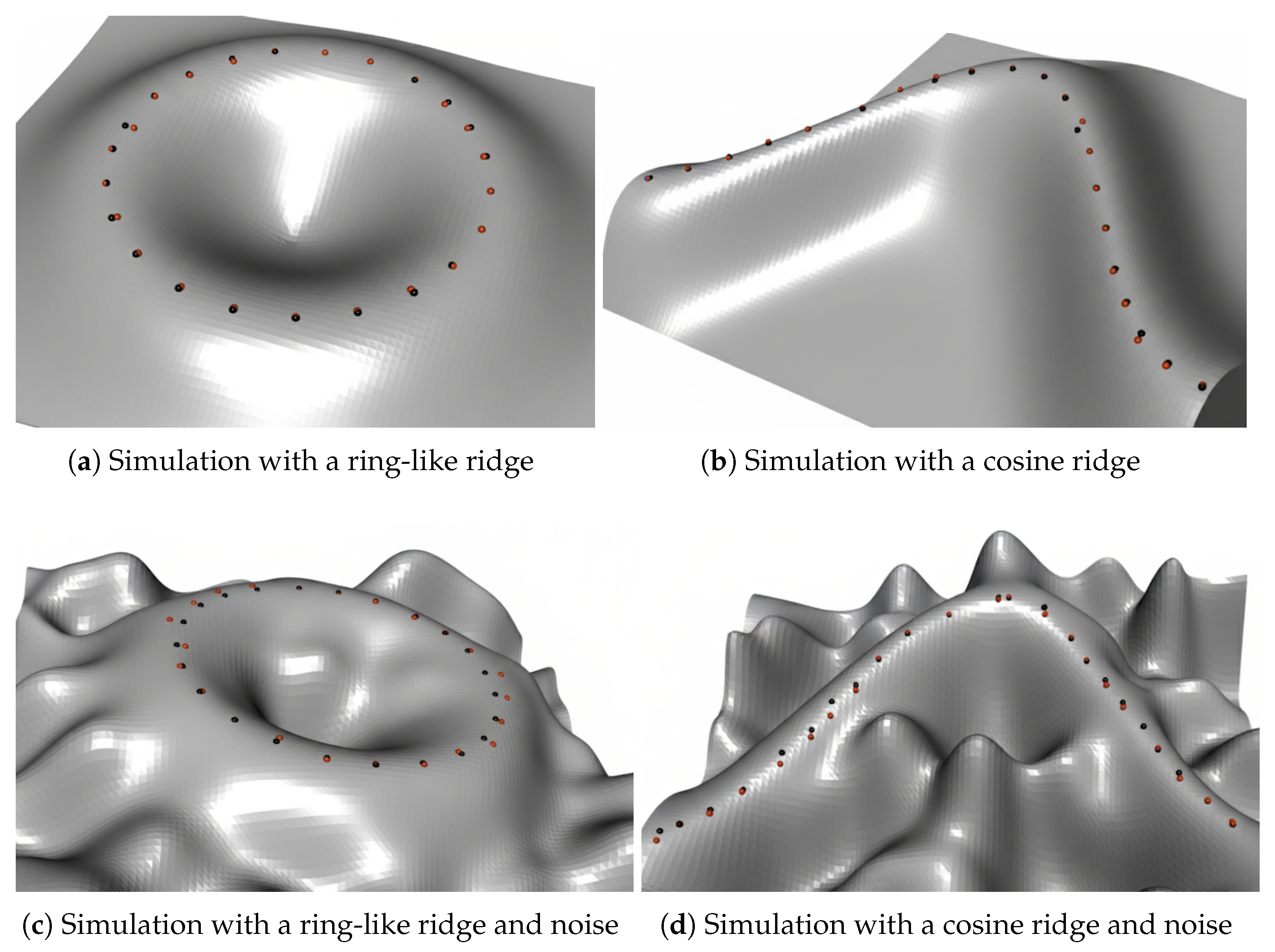
Section 3.1. The evaluation utilizes two primary shapes, a ring-like curve and a cosine curve, depicted in
Figure 5a and
Figure 5b, respectively. For each shape, the analytically defined true curve is compared against the curve estimated by our algorithm. Furthermore, to assess the method’s robustness, varying levels of random noise were added to the surfaces to analyze the impact on performance.
3.2.1. Create the Surface
The surfaces for the simulation were constructed on a
grid in the
x-
y plane, spanning a width of two arbitrary units. To form a ring-like ridge, the height (
z-coordinate) at each grid point was determined by the following Gaussian function:
where
represents the Euclidean distance from any point
to the grid’s center. This formulation ensures that the true ridge is a circle of radius 1 centered on the grid, with a constant height of
. A visualization of this shape, along with the true curve marked by black dots, is provided in
Figure 5a.
A Gaussian random field is a mathematical tool used to generate surfaces with natural-looking, random textures, like bumpy terrain or noisy data. A weighted Gaussian random field adds a layer of control, allowing you to vary the amount of randomness across the surface to make some areas rougher while keeping others smooth. To simulate shapes similar to ones in
Figure 3, noise generated from a weighted Gaussian random field was added to the surface. For the ring-like ridge, the weight function is defined as
, where
. This distance-based weighting scheme is created based on Gaussian Radial Basis Function (RBF), a standard method for creating a smooth, localized field of influence [
42]. It is designed to preserve the main ridge structure, regardless of the noise level in the surrounding area. Specifically, points located on the ridge have
, which results in
and a maximum weight of
. Points close to the ridge have small values of
D and therefore also have high weights. As a result, even when significant noise is applied to the entire surface, the ridge itself remains well-defined, and the points near it are not greatly displaced. An example of the noisy ring-like shape, with the true curve shown as black dots, is depicted in
Figure 5c.
A similar process was used to create a cosine-shaped ridge. Its height (
z-coordinate) is defined by the equation:
This formula yields a true ridge following a cosine path at a constant height of
, as shown in
Figure 5b. To add noise, the same weighting approach was applied, with the weight function
now using
. This ensures the cosine ridge remains intact amidst the noise, as illustrated in
Figure 5d.
3.2.2. Estimate the Ridge Curves
In this simulation study, the analytical coordinates of the true ring-like ridge curve and the cosine ridge curve can be determined. When the ring-like curve is projected onto the
x-
y plane, it forms a circle that satisfies the equation
. The third dimension,
z, is held constant at the value obtained when
in Equation (
4). Thus, the coordinates of the ring-like curve are given by:
Similarly, the projection of the true cosine ridge curve onto the
x-
y plane is the line
. The
z-coordinate is also held constant at the value obtained when
in Equation (
4). Thus, the coordinates of the cosine ridge curve are given by:
The algorithm from
Section 3.1 estimates these curves. As the geometry information on the surface with noise is rather complex, the initial seed was placed manually using the IDAV Landmark Editor software. As noted in Step 3 of the method, the estimation relies heavily on curvature calculations, which in turn depend on the size of the local neighborhood used. We therefore investigated the influence of this neighborhood radius, denoted
. The top row of
Figure 5 shows the identified curves (red dots) versus the true curves (black dots, from Formulas (
6) and (
7)) on the noise-free simulated shapes.
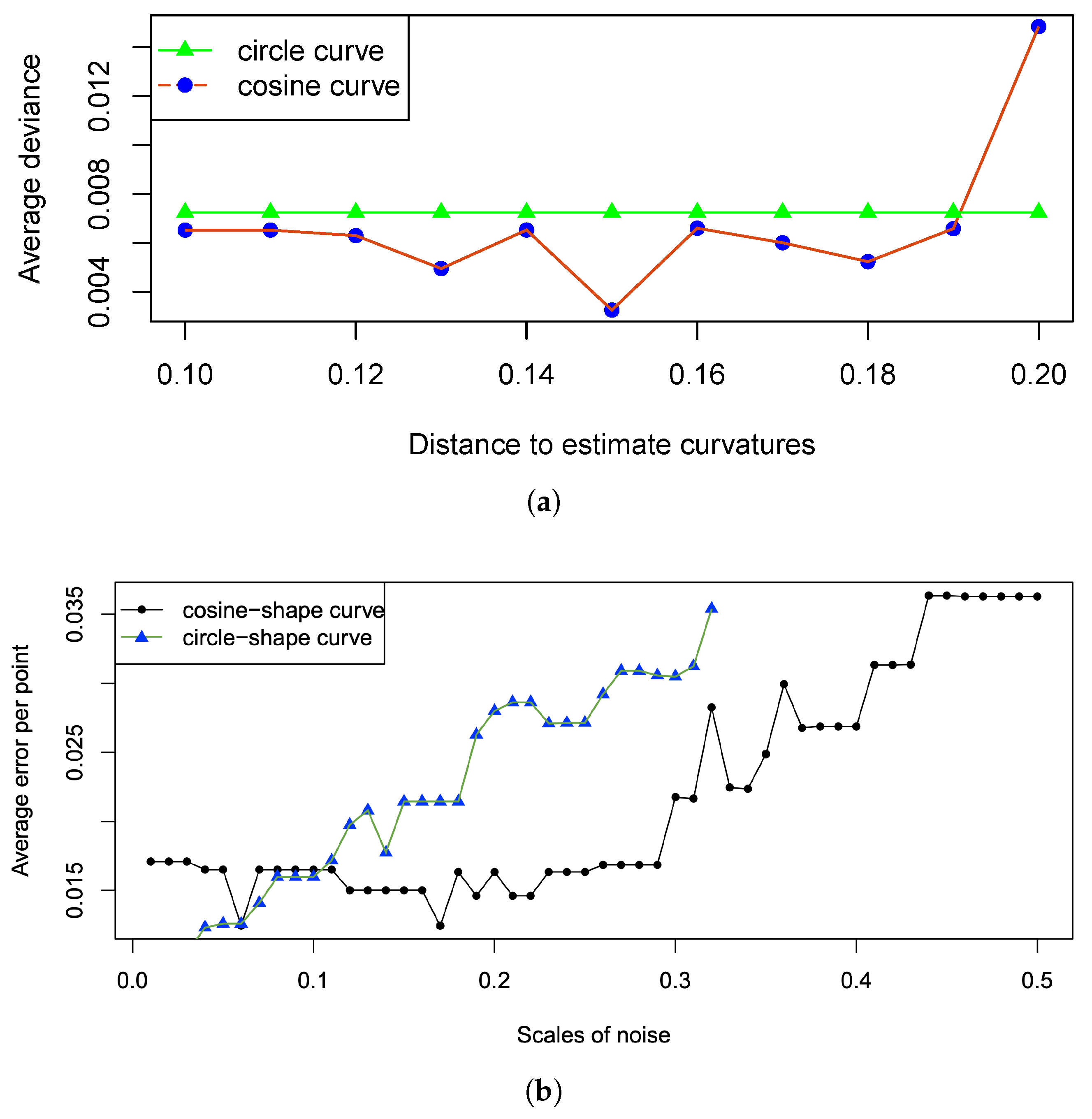
The relationship between the average estimation error and the neighborhood radius
is plotted in
Figure 6a. For these two shapes, the choice of
in the range of
has a minimal impact on the results (less than 0.3% variation). Consequently, we selected a radius of
which has the smallest average deviance on the cosine curve for the remainder of the simulation. The effect of noise on estimation accuracy is shown in
Figure 6b (right). The second row of
Figure 5 illustrates the impact of a large, 40% noise level. While noise affects the circular curve more significantly, the average deviance per point remains low, at just 3.5% even with a 50% noise level.
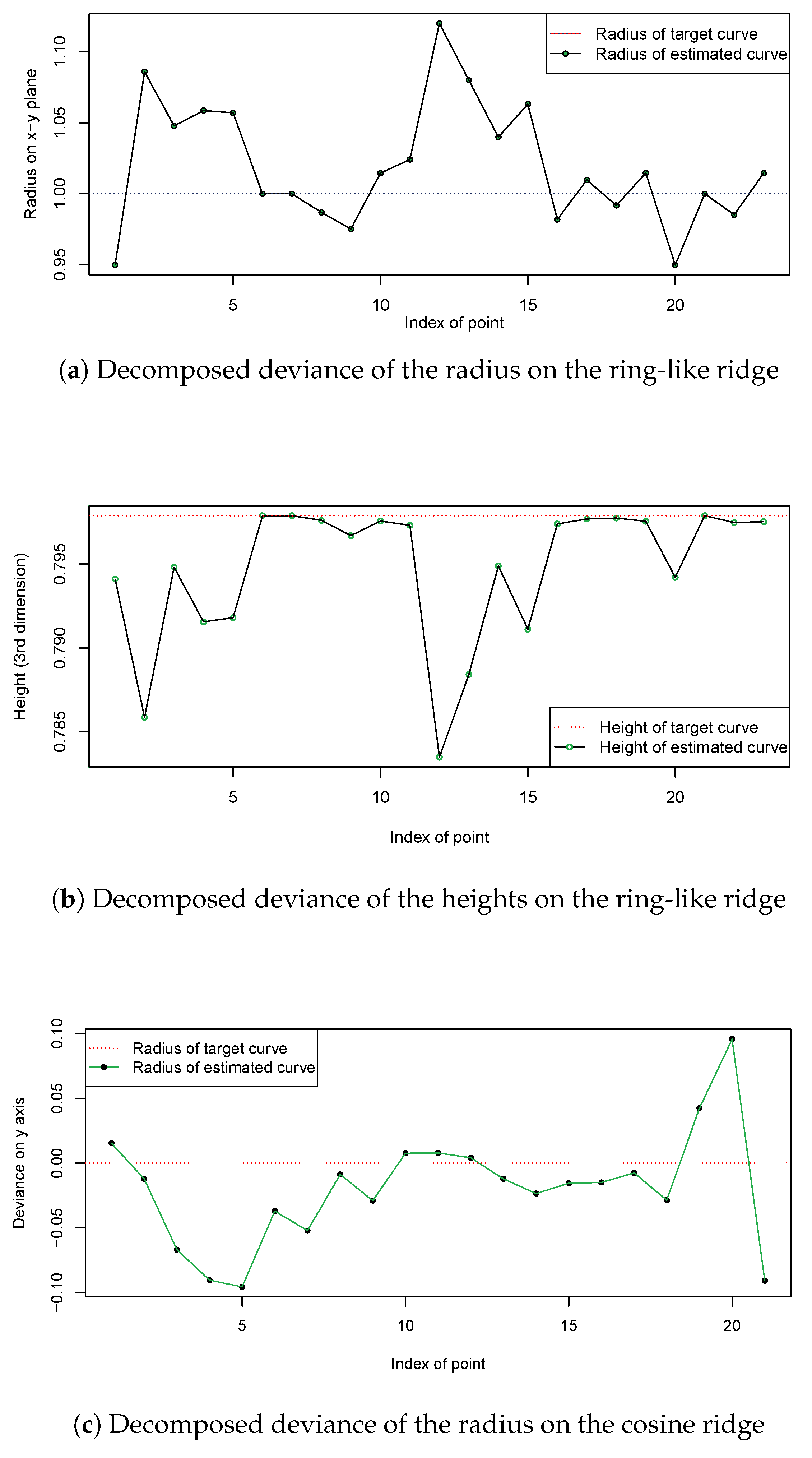
Figure 7 details the decomposition of the estimation error for the curves shown in
Figure 5. For the circular curve, the deviance is broken down into radius and height components (
Figure 7a,b). For the cosine curve, since the x-coordinates are matched, the deviance is decomposed into the second and third dimensions (
Figure 7c,d). Even with substantial noise, the error in the third dimension is at most 0.5%, while errors in other dimensions are around 2.5%, which is quite small.
In summary, the method performs well in identifying curves from sparse landmarks, with errors remaining within an acceptable range. As explained in
Section 3.1, the algorithm can achieve an accurate estimation as long as significant noise is not present in the immediate vicinity of the curve.
4. Transmission of 3D Point Cloud
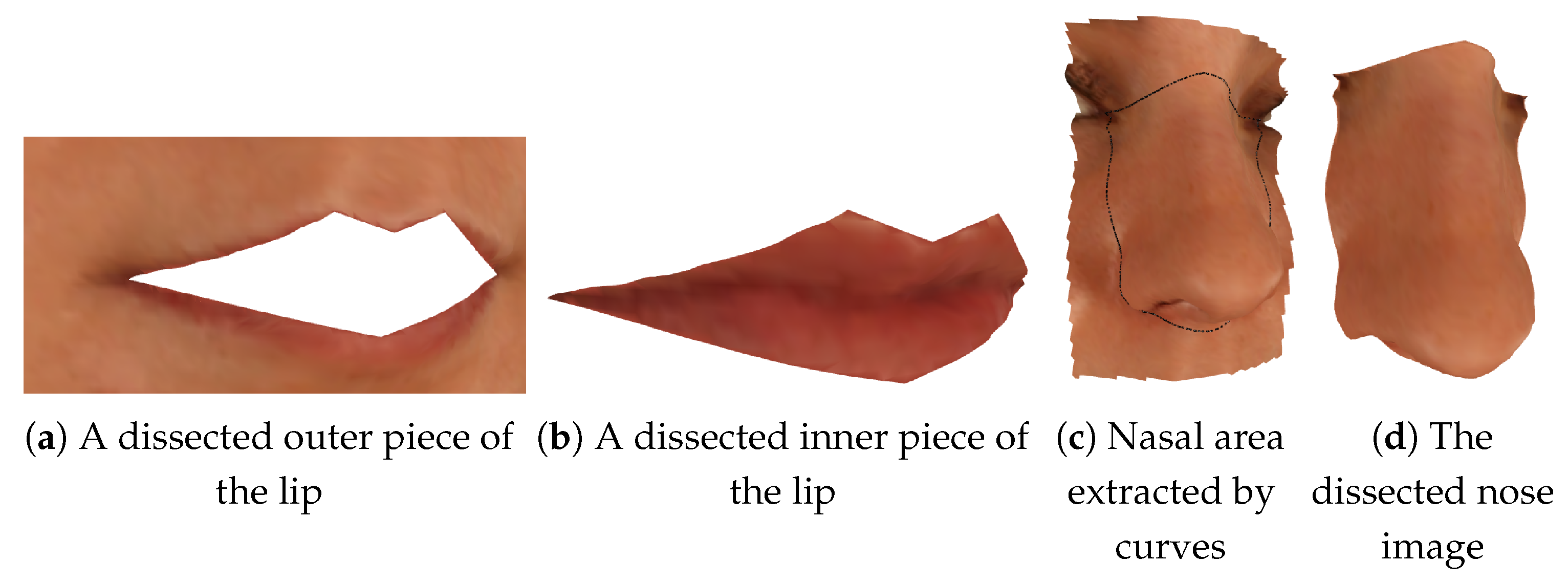
In this section, we use the hybrid transmission scheme to investigate the efficiency and robustness to transmit 3D extracted features. A zero-loss dissection algorithm was introduced by reconstructing the triangulation along the estimated curves [
38]. The fundamental strategy of the dissection method involves eliminating triangles intersected by the specified 3D curve and subsequently reconstructing the mesh along the cut. As shown in
Figure 8a,b, it produces two complete pieces without throwing any information away.
Figure 8c shows an example of the nasal area characterised by the estimated curves and
Figure 8d shows the 3D nasal area dissected by the algorithm.
4.1. Model Description
The proposed adaptive model is developed based on Deep Joint Source–Channel Coding (DeepJSCC) [
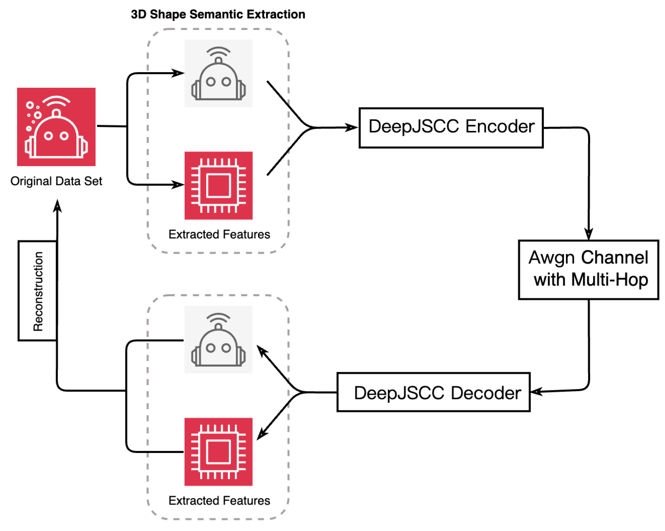
43]. As illustrated in
Figure 9, the overall architecture consists of three main components: the encoder, the channel module, and the decoder. The encoder employs a sequence of convolutional layers, activation functions, and a self-attention mechanism, which enables adaptive feature extraction according to the channel quality. In addition, we further employ the 2-D Fast Fourier Transform (FFT) on the obtained matrices (i.e., transformed from the original 3D data) to generate different frequency outputs before the attention mechanism. The intuition behind the integration of the self-attention mechanism is it allows the model to selectively emphasize informative point-to-point and region-to-region relations in the feature space, thereby improving robustness against channel distortions and improving reconstruction of fine-grained geometric structures. We also provide a detailed architecture about our encoder and decoder in
Figure 10.
In this work, the input tensor is generated from preprocessed numerical point cloud data. The encoder employs a sequence of convolutional layers, activation functions, and a self-attention mechanism, which enable adaptive feature extraction according to the channel quality (SNR). The output feature tensor has a shape of with , where H and W are reduced spatial dimensions. This feature tensor can be regarded as the baseband representation of the transmitted signal.
The encoder output is reshaped into complex-valued signals for channel simulation. We adopt a three-hop amplify-and-forward (AF) relay network, where each hop introduces additive white Gaussian noise (AWGN) determined by the given signal-to-noise ratio (SNR). Specifically, the received signal is modeled as
where
denotes the encoded complex signal and
is the complex Gaussian noise.
The noisy received signal is converted back into a real-valued feature tensor and fed into the decoder, which mirrors the encoder architecture with transposed convolution layers, activation functions, and a self-attention mechanism. This enables the decoder to adapt its reconstruction process based on channel quality. The final output is a reconstructed image tensor.
4.2. Training Strategy and Metrics
The primary model used is a regular DeepJSCC under the conditions of bandwidth ratio = 1/6. In addition, we further employ the 2-D FFT on the obtained matrices (i.e., transformed from the original 3D data) to generate different frequency outputs before attention mechanism. We adopt a fine-tuning strategy by loading pretrained weights and the parameters is updated using the Adam optimizer with a learning rate of . The maximum number of epochs is set to 100.
To comprehensively assess model performance, we adopt the Peak Signal-to-Noise Ratio (PSNR) metric to evaluate the objective reconstruction quality. We first transform the 3D point cloud data into a 2D form, i.e., if there exists point cloud data on a 3D coordinate, record its coordinate position as valid data in the 2D matrix. By this means, we make it suitable for model input and evaluation. The model is evaluated under AWGN channels with varying SNR values.
4.3. Results and Findings
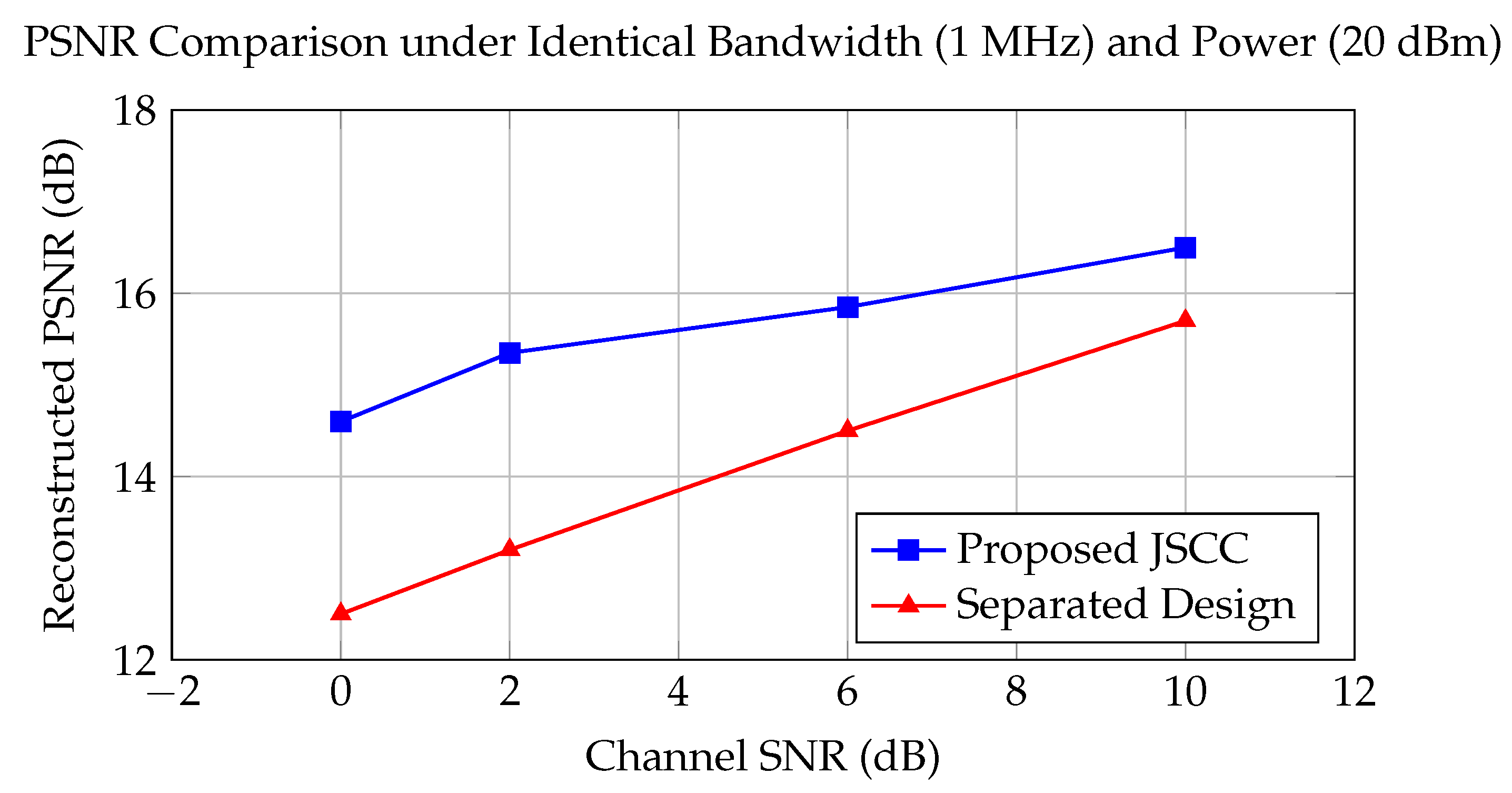
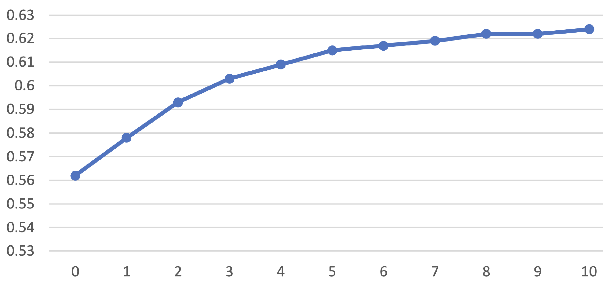
The simulation of transmitting 3D images was based on our own database which contains 82 facial images. The lip feature of each image was extracted and each lip image contains roughly 500 points. The performance of the proposed communication framework was evaluated under different channel SNRs in
Figure 11. The results show that, when the SNR increases from 0 dB to 10 dB, the reconstruction quality improves with an average PSNR gain of approximately
dB. The reason lies in the fact that the joint codec can better match the coding rate between the source and channel, and thus the reconstructed results are more robust compared to separate design. In our experiment, it was shown that the average performance improvement across SNR = 0–10 dB was about 1.5 dB, and the advantages of the proposed scheme were more pronounced in poor channel conditions. This is also in line with the expected performance of the joint source channel coding scheme in other literature [
43,
44].
Figure 12 shows the simulation results of structural similarity index measure (SSIM) across SNR = 0–10 dB. To calculate the SSIM value, we transformed the original 3D point cloud data into a 2D matrices, which had the same format as the image. The SSIM values ranged from 0.56 to 0.62.


