Article

Smartphone-Based Edge Intelligence for Nighttime Visibility Estimation in Smart Cities

1
Academy of Military Science, Beijing 100850, China
2
Digital Intelligence and Simulation Collaborative Innovation Center, Hunan Institute of Advanced Technology, Changsha 410000, China
*
Author to whom correspondence should be addressed.
Electronics 2025, 14(18), 3642; https://doi.org/10.3390/electronics14183642
Submission received: 26 August 2025 / Revised: 9 September 2025 / Accepted: 11 September 2025 / Published: 15 September 2025
(This article belongs to the Special Issue Advanced Edge Intelligence in Smart Environments)

Abstract

Impaired visibility, a major global environmental threat, is a result of light scattering by atmospheric particulate matter. While digital photographs are increasingly used for daytime visibility estimation, such methods are largely ineffective at night owing to the different scattering effects. Here, we introduce an image-based algorithm for inferring nighttime visibility from a single photograph by analyzing the forward scattering index and optical thickness retrieved from glow effects around light sources. Using photographs crawled from social media platforms across mainland China, we estimated the nationwide visibility for one year using the proposed algorithm, achieving high goodness-of-fit values (R2 = 0.757; RMSE = 4.318 km), demonstrating robust performance under various nighttime scenarios. The model also captures both chronic and episodic visibility degradation, including localized pollution events. These results highlight the potential of using ubiquitous smartphone photography as a low-cost, scalable, and real-time sensing solution for nighttime atmospheric monitoring in urban areas.

1. Introduction

Atmospheric aerosols, increasingly influenced by anthropogenic activities, play critical roles in Earth’s climate system and significantly affect air quality and human health [1,2,3]. Visibility, a crucial indicator of atmospheric clarity and aerosol loading, has shown a continuous decreasing trend globally due to increased anthropogenic particulate matter emissions in these years [4,5,6]. The significantly deteriorated visibility level harms human health and increases risks in daily mortality, raising an urgent need for constructing a diurnal cycle of visibility level monitoring. The appearance of visibility degradation is due to the presence of particulate matter that scatters light rays, which forms the basis of visibility monitoring.
Standards instrumentation for visibility monitoring includes electro-optical sensors such as nephelometers, measuring the light scattering coefficient, and transmissometers, determining the light extinction coefficients [7]; these measurements are converted to meteorological optical range, often termed reference visibility, using Koschmieder’s equation [8]. While these approaches serve as ideal tools and established benchmarks, the high cost of these instruments restricts their deployment, and hence, they are scarce. Aside from these cost-prohibitive approaches, remotely sensed images are increasingly being used as the data source for monitoring visibility, including nighttime applications [9,10]. These studies typically relate satellite aerosol optical depth or radiance reductions over light sources to visibility values, providing accurate visibility estimates for large coverage. However, satellite-based approaches are inherently constrained by factors including cloud contamination, the presence of missing values, and relatively low update frequency (revisit frequency), making it difficult to produce a real-time and complete observation record in space and time.
Limitations of traditional visibility monitoring approaches—namely the cost and sparsity of ground stations and the temporal constraints of satellite data—have motivated exploration of alternative methods, particularly those utilizing camera imagery. For instance, the existing highway cameras or vehicle headlamps have been attempted to estimate the atmospheric visibility value [11,12,13]; webcam images are explored as an alternative way to measure visibility levels with a series of image processing techniques. Methods employing such digital photographs generally capture embedded visual features (e.g., color contrasts, texture contrasts, and saturation density) that reflect scattering effects and then construct mapping functions between these visual features and visibility measurements. In addition to these fixed camera sensors, several reports have also suggested a new paradigm for monitoring that utilizes portable and low-cost sensors to provide data in near real-time [14,15], with the smartphone acting as an accessible and ubiquitous sensor. Consequently, smartphone photographs have been discussed as being a potentially promising atmospheric sensor in a crowdsensing way [16,17,18,19]. These methods, however, are primarily limited to daytime conditions; low light, poor quality, and impaired scenes present challenges for visibility monitoring after dark [20].
An earlier study by Narasimhan and Nayar [21,22] demonstrated that glow effects observed around light sources (e.g., streetlamps and car lights) at night are prominent manifestations of multiple scattering by particulate matter. They established that the spatial distribution of this scattering light intensity, as captured by a camera, represents the atmospheric point spread function (APSF) for that light source. The APSF describes how the intensities around light sources are spread along with the angular, and how the shape of the glow is varied by weather conditions. With the APSF, two key weather parameters (i.e., optical thickness and forward scattering parameter) can be approximated, enabling visibility estimation. This foundation work provides a physics-based framework for analyzing nighttime imagery and advances the understanding of nighttime light scattering by atmospheric particles [21,23]. However, their proposed approach requires known reference information (e.g., distance to light sources) and involves computationally intensive optimization (tens of minutes per image) to retrieve APSF parameters, precluding real-time applications. Subsequent research has thus focused on improving efficiency. For example, inspired by the successful application of the standard haze model [24,25], several studies incorporated the glow effect into image formation models, often using APSF parameters to improve nighttime image dehazing [26,27]. Although these methods efficiently model or mitigate glow effects for visual enhancement, they were primarily designed to generate visually clear images and typically do not yield highly accurate and consistent measurements of nighttime visibility. Hence, a significant need persists for a novel algorithm capable of accurate, real-time nighttime visibility estimation from single images.
In this paper, we propose a novel algorithm for deriving two weather indices, namely optical thickness index and forward scattering index, from smartphone photographs to estimate nighttime visibility. Glow effects around light sources (glow layer) are first separated from the input smartphone image, and thus APSF can be estimated from the separated glow layer. The optical thickness index and forward scattering index are subsequently derived by fitting the estimated APSF profile with an asymmetric generalized Gaussian distribution (AGGD) model. Finally, we estimate visibility using these two derived parameters. The algorithm’s performance in estimating the nighttime visibility is validated through a national-scale case study using smartphone images crowdsourced from the Internet.
This paper is structured as follows: Section 2 reviews the physics of multiple light scattering under various weather conditions, which is the cause of glow effects around light sources. Section 3 details the methodology for extracting atmospheric parameters from smartphone images, including APSF estimation and AGGD model fitting, and presents the model developed for final visibility estimation. Section 4 presents the evaluation of the model-fitting performances and the results of visibility estimation. The discussion is presented in Section 5, and perspectives and conclusions are also included.

2. Nighttime Multiple Light Scattering Under Weather Conditions

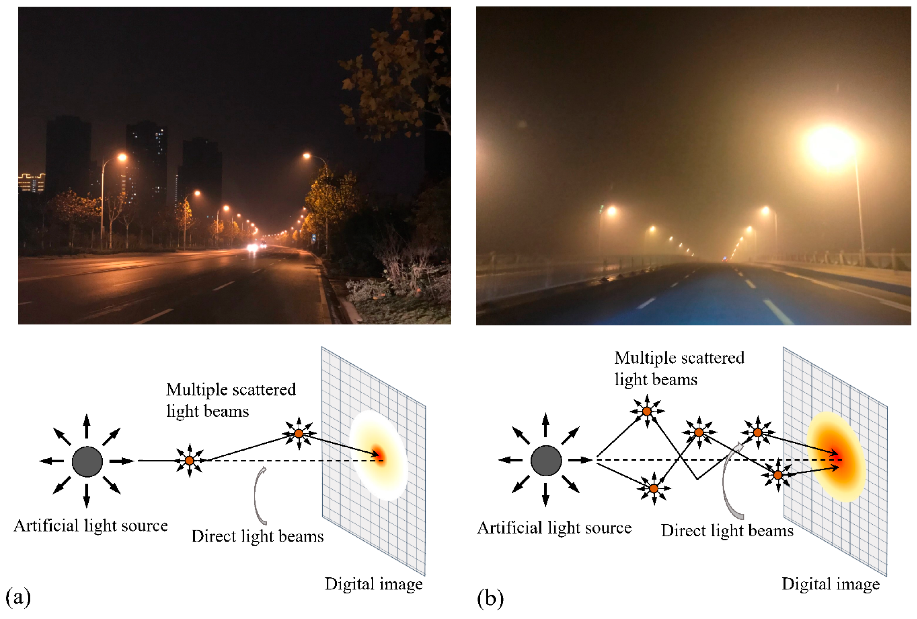
Atmospheric aerosols participate in light scattering and hence result in blurred vision. This reduction in clarity provides visual cues related to the intensity of scattering, which, in turn, can be used to infer atmospheric conditions, particularly aerosol loading. Virtually all methods for retrieving scattering properties rely on the assumption of single scattering dominance, which may be broken at nighttime when multiple scattering is prevalent. Multiple scattering refers to the light being scattered multiple times in various directions and is the dominant cause of the prominent glows around artificial light sources. On a clear night, relatively few aerosols participate in the multiple scattering process, resulting in small and concentrated glow effects around light sources (Figure 1a). Conversely, on a heavily hazy night, a large number of aerosols are engaged in the multiple scattering process, leading to the formation of prominent, intense, and widely dispersed glow effects (Figure 1b).
The prominent glow around artificial light sources at night arises mainly from two causes: one is the direct transmission of light, and the other one is the multiple light scattering, i.e., light becomes scattered several times in different propagation directions. Typically, the multiple scattered light is measured by the change in light flux through an infinitesimal volume by the Radiative Transfer Equation (RTE) [28,29], which is expressed as follows:
μ I T + 1 μ 2 T I μ = I T , μ + 1 4 π 0 2 π 1 + 1 P c o s α I T , μ d μ d ϕ
In Equation (1), I ( T , μ ) denotes the light intensity of a point source, which is determined by the cosine of the scattering angle c o s α = μ μ + 1 μ 2 1 μ 2 c o s ( ϕ ϕ ) ) and the general phase function P c o s α . The scattering angle α is the angle between the scattered direction ( μ = c o s θ ) and the incident direction ( μ = c o s θ ). T = σ × R is the optical thickness of the atmosphere, denoting the light attenuation in the medium, and is determined by distance R and extinction coefficient σ . When taking various weather conditions into account, the general phase function in Equation (1) is usually modeled by the Henyey–Greenstein phase function [30], which is expressed as follows:
P c o s α = 1 q 2 1 2 q c o s α + q 2 3 2
where q [ 0,1 ] is the forward scattering parameter, which varies under different weather conditions (e.g., clear air, mist, fog, or rain). The larger the particle size, the greater the forward scattering parameter. When q approaches 0, the scattering tends to be isotropic; when q approaches 1, the scattering tends to be anisotropic with the scattered direction to be α = 0 . An approximate value of the forward scattering parameter q under various weather conditions is listed in Table 1 [31]. From Equations (1) and (2), we can infer that the multiple light scattering depends on three factors: the optical forward scattering parameter [ q ], the optical thickness [ T ], and the scattered angle [ α ]. Suggested in [21], this angle-dependent anisotropic model can be loosened to an angle-free model. The modified angle-free model constitutes the atmospheric point spread function (APSF).
As discussed above, the glow is the addition of direct transmission and multiple scattering of light in the night environment. The direct transmitted light is determined by the intensity of each artificial light source; the multiple scattered light is intimately influenced by the weather conditions (i.e., optical thickness [ T ] and forward scattering parameter [ q ] ), forming various shapes of the glow that can be measured or computed by the APSF. These provide the basis for discriminating against various atmospheric conditions.

3. Nighttime Visibility Estimation

As the glow present in the night image (i.e., two-dimensional glow) is a projection of the real-world APSF onto the image plane, the key factors (optical thickness and forward scattering index) for measuring the nighttime visibility level are unable to be retrieved directly. Nevertheless, the nighttime visibility can still be estimated in an indirect way by deriving the weather indices, optical thickness index (OTI), and forward scattering index (FSI) from smartphone photos.
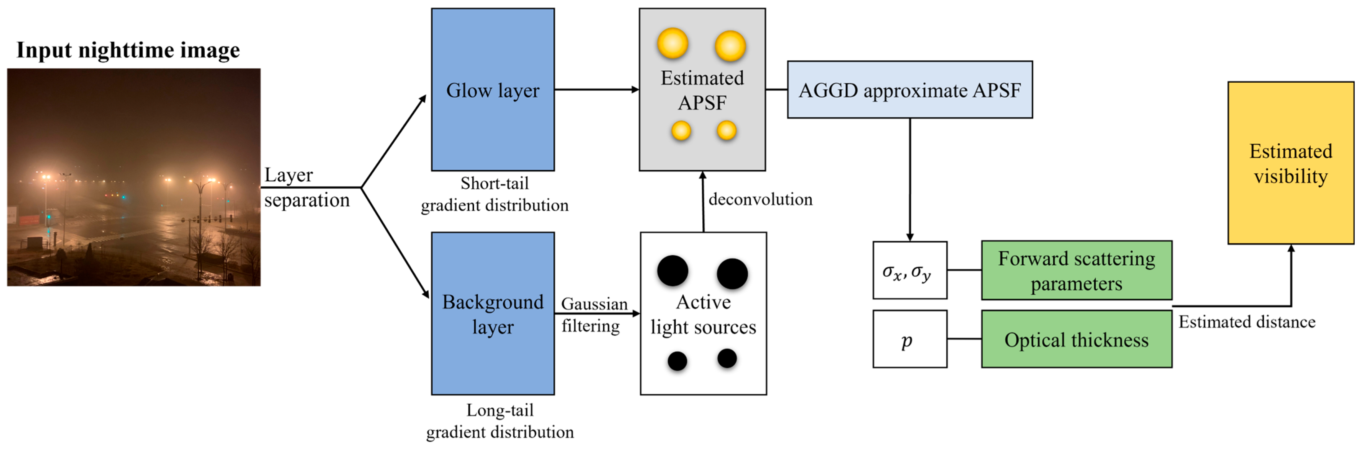
To derive a weather index from a smartphone photo, we were inspired by the common-sense observation that the naked human eye can easily distinguish an ambient environment at night using visual properties (e.g., size and shape of the glow) without additional knowledge. A schematic overview of the proposed algorithm is shown in Figure 2. Given a smartphone photo, we first separate the layer from photographs that only contain the glow effects, i.e., the glow layer, by assuming the photographs with haze are a linear combination of multiple layers (see Section 3.1). APSF presents how the intensity around the light source propagates and diminishes, estimated from the area where the artificial light source is detected (see Section 3.2). The APSF is then fitted by an asymmetric generalized Gaussian distribution (AGGD) filter [23,32]; two weather indices, that is, the optical thickness index and the forward scattering index, can be calculated from the AGGD parameter [23] (see Section 3.3). Using weather indices, the visibility distance can then be estimated using the proposed model (see Section 3.4).

3.1. Nighttime Haze Model with Glow Layer Separation

As shown in Figure 1, particulate matter participates in the scattering and plays a significant role in booming the glow that is observed around light sources. The impaired nighttime scene is often characterized via the standard nighttime haze model [27]:
I x = J x t x + L x 1 t x + G ( x )
where I ( x ) is the intensity of the hazy image is observed and is the result of a linear combination of three components (i.e., direct attenuation, local air light, and the glow). The first two components constitute the nighttime image in a clear view, while the last component characterizes the glow effects when haze is presence. J ( x ) t ( x ) , the direct attenuation, describes the scene radiance and its decay in the atmosphere; the former, J , is the scene radiance when no haze is observed; and the latter, t , represents the transmission map that denotes the light attenuation process from farthest to the observer. L x 1 t x describes the local airlight, resulting from the localized environmental illumination and L x is the local atmospheric light. G is a glow layer, characterizing the glow effect around light sources. Thus, the nighttime hazy image can be regarded as the addition of two image layers (the clear layer and the glow layer).
In accordance with Li et al. [27], the glow layer and clear layer of the nighttime image show distinct disparity in their texture gradient histograms, because the hazy weather imposes the dominant smoothing effect around the light sources, making the gradient histogram of the glow layer close to a short-tailed distribution, while giving the gradient histogram of the clear layers a long-tailed distribution. We exploit this feature and employ the layer separation method, in which two layers that hold significant differences in texture gradient histograms can be separated by approximating the probabilities [33]. As discussed above, J x t x + L x ( 1 t ( x ) ) forms the clear night view, namely de-glow layer, while G ( x ) , the glow layer, presents the glow effect. Following [33], two layers can be decomposed by constructing a probability distribution on each gradient histogram:
P g x = 1 2 π σ 1 2 e x 2 σ 1 2
P c x = 1 z max e x 2 σ 2 2 , ϵ
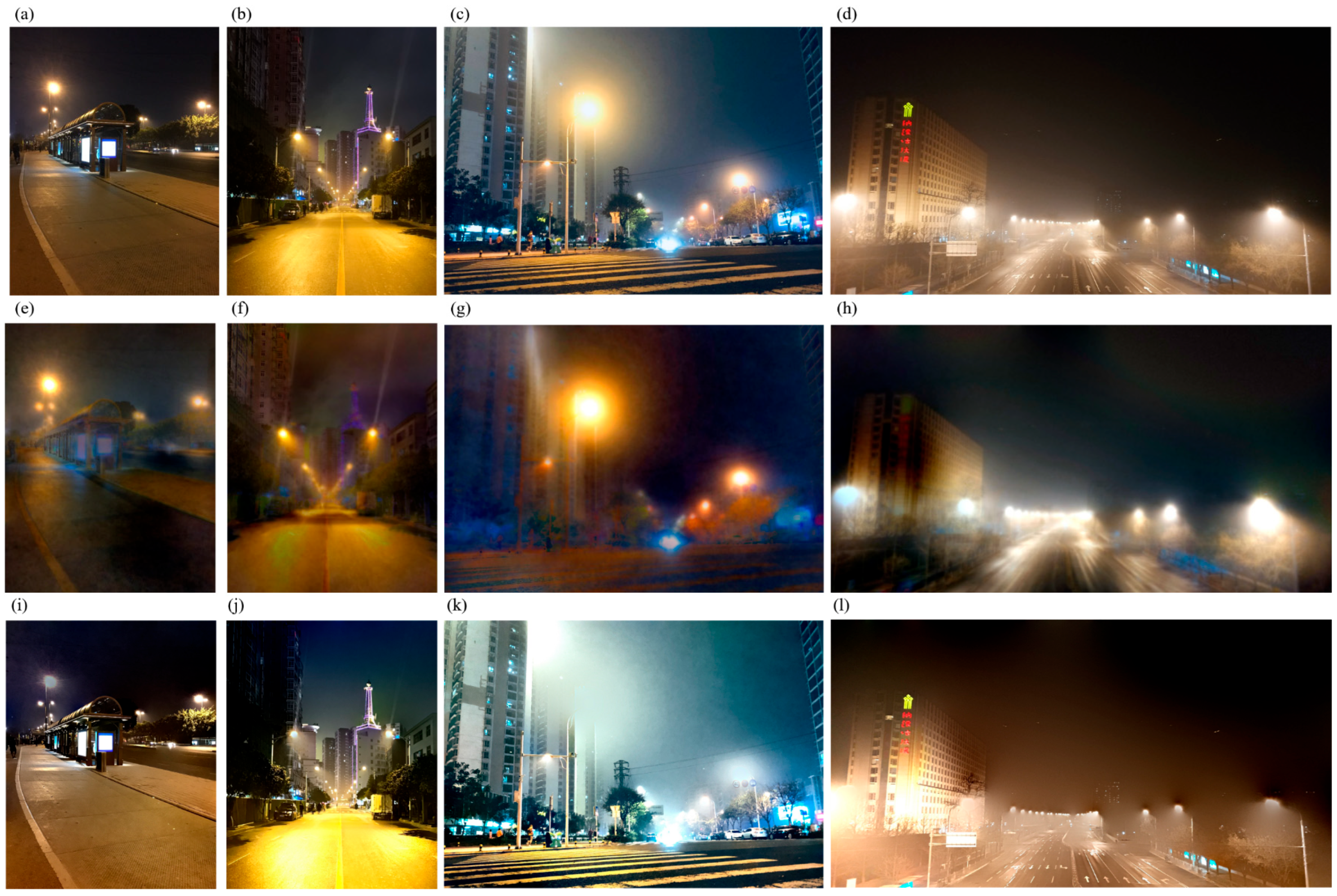
where P g x represents short-tailed Gaussian distribution with x is the gradient value of the glow layer. σ 1 is a very small value, making the Gaussian narrow and quickly fall off. P c x is a long-tailed distribution; σ 2 is also a small value, controlling the shape of the Gaussian. z is a normalization factor; ϵ = 1 e 6 is a sparse penalty term that prevents P 2 ( x ) from quickly dropping to zero. The optimal solutions can be solved by standard optimization methods. Examples of separated glow layers and de-glowed layers of different nighttime photographs under various weather conditions are shown in Figure 3.

3.2. APSF Estimation

The glow effects around light sources arise from direct transmission and multiple scattering, which are governed by the joint effect of light-source intensity and multiple scattered lights. APSF that presents at nighttime photographs can be obtained by analyzing the approximately ideal isolated light sources.
G x = L a x A P S F
where G is the glow layer and denotes a convolution operator. L a is the locally active light source image that can be estimated through high-pass filtering or a standard moving window detection.

3.3. Weather Indices Retrieval by AGGD Filter for APSF

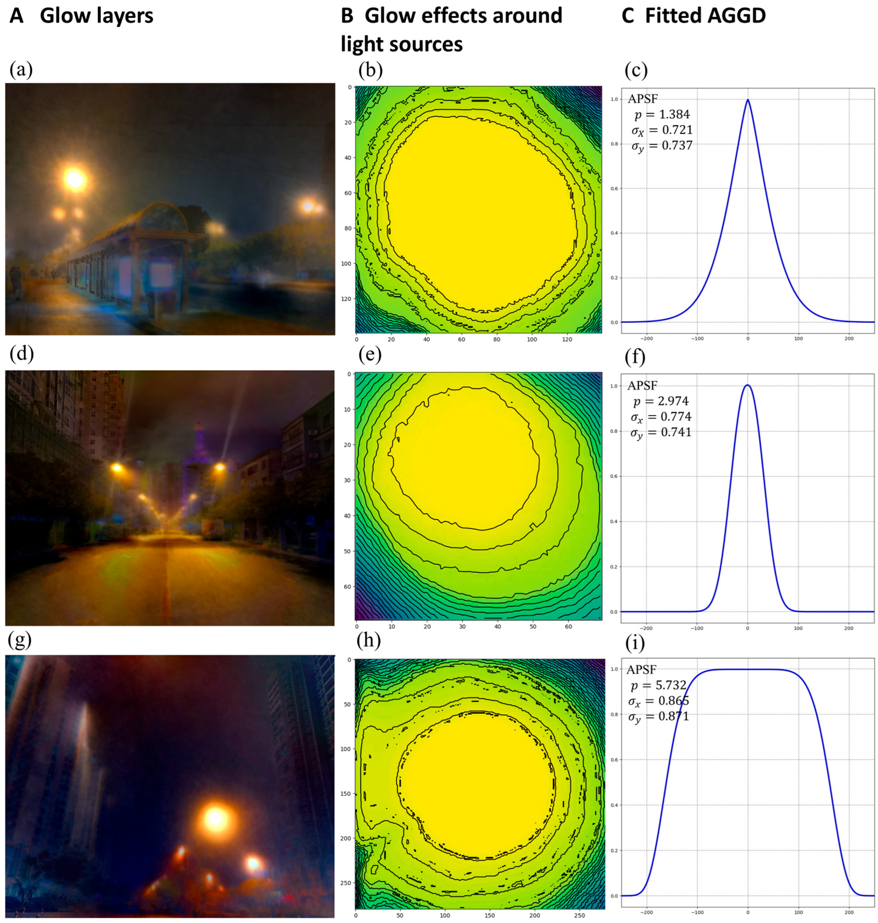
As shown in Section 2, the shape of APSF varies under different weather conditions. In addition, the projection of the APSF onto the image plane manifests as a two-dimensional glow. This glow often appears as an asymmetric, radially decaying intensity pattern centered around the light source (Figure 4B), whose characteristics are dictated by atmospheric conditions. Ideally, a solution of APSF (optical thickness and forward scattering parameter) can be obtained by numerical simulations [21,22]. However, solving APSF with numerical methods may not converge in all situations (all levels of hazy conditions) [23,27]. Alternatively, one possible approach is to use Gaussian distribution to fit the profile of APSF, which is an analog to the standard solution for point spread function (PSF) in the astronomical and satellite image deblurring literature (see, for example, [34,35]) and assumes that PSFs can be treated as symmetric objects with a known precise shape. In practice, however, the assumption of symmetric light scattering and a known shape of light sources is always unreasonable for smartphone photographs because of the various shooting angles and the unknown relative positions and distances to light sources.
To model the shape of the APSF, we employ the asymmetric generalized Gaussian distribution (AGGD) filter [36], a flexible function capable of representing a wide range of distribution shapes and thus accommodating the majority of real-world conditions. The AGGD is defined as follows:
A G G D x , y ; σ x ,   σ y , p = e x μ x 2 + y μ y 2 p 2 4 Γ 2 1 + 1 p A p ,   σ x A p , σ y ,         x , y R
where x ,   y is the coordinate of a point of a glow region. p is the shape parameter, which controls the distribution’s kurtosis and reflects the extent of multiple scattering; σ x ,   σ y are scale parameters representing the spread in the horizontal and vertical directions, and μ x and μ y represent their mean values, respectively. Γ ( · ) is the gamma function, Γ z = 0 x z 1 e x d x . A p ,   σ = [ σ 2 Γ 1 p / Γ 3 p ] 1 2 is a scale function. A nonlinear least-squares fit computes the AGGD approximation to an APSF as follows:
m i n A P S F x , y A G G D x , y 2
This minimization can be obtained with any standard optimization program. We note that, in practice, solutions for AGGD may sometimes not be unique. An average operation for AGGD parameters after having an anomalous detection of solutions (including abnormal variances and high costs) is generally sufficient to derive reasonable results. Examples of APSFs on the glow layers and the fitted AGGD are presented in Figure 4.
Because the APSF extracted from a glow layer is often non-unique due to the presence of multiple light sources. Putting the single glow layer as a unity to directly estimate AGGDs for multiple APSFs may take several minutes and is indeed unnecessary to do, given the uninformative nature of the outer regions of the APSF profile. A subtraction operation, therefore, can be applied to effectively reduce the computational time used for distribution approximation. To do this, we first chop up the glow layer into non-overlapping sub-windows; each sub-window contains only an APSF, and the size of the sub-window is determined by a hard threshold, turning off all pixels whose ratio of the light intensity to the local maximum (intensity of the brightest center) is under 80%. We then discard the outer regions of each sub-window, leaving essentially an APSF contour not contaminated by the background, and compose the final results from the APSF of each inner sub-window.
The AGGD (Equation (7)) enables simulating APSF under various atmospheric conditions by adjusting its parameter ( p , σ x ,   σ y ), thus serving as a proxy for quantifying multiple scattering effects. This is consistent with observations (Figure 4C)—as atmospheric particulate matter becomes denser, the extent of the glow increases, typically reflected by increasing the shape parameters. Suggested by previous research [23,26], AGGD parameters ( σ x ,   σ y , p) and weather parameters can be linked by a linear mapping. We follow the proof presented in [23]; two weather indices, optical thickness index (OTI) and forward scattering index (FSI), can be estimated from AGGD parameters as follows:
O T I = k T ,         k R +
σ x = 1 F S I F S I ,         σ y = 1 F S I F S I
where k is a fitting parameter. We note that σ x and σ y should be close, although values of them are naturally different. Figure 4 shows plots of the fitted AGGD from APSF and the corresponding glow layer under three distinct weather conditions.

3.4. Visibility Estimation Model

The forward scattering index ( F S I ) and optical thickness ( O T I ) are coherently related with visibility [37]. In this study, we only consider the nighttime photographs with haze; it is natural to assume that the forward scattering parameter should be close (as shown in Table 1). As shown in Section 2, the optical thickness parameter p , which refers to the ratio of intensity loss of incident light due to the scattering process in the atmosphere, is related to the visibility value:
T = β R
β 3.912 V
where β is the atmospheric extinction coefficient; V is the visibility range; and R is the distance from the observed light sources to the observer. The relative distance can be measured by any object detection-based distance estimation technique [38], assuming that the real object size is approximately the same (see Supplementary Information S3). As suggested in [39], a simple linear regression can be employed to model the relationship between visibility and the weather parameters. By combining Equation (8) with Equations (11) and (12), the nighttime visibility model based on the estimated optical thickness index (OTI) is given as follows:
O T I = k × R × 3.912 V
where a is the fitting parameter. Equation (12) indicates, once the distance R is given, that the index O T I can be calculated; therefore, the visibility can be estimated through a linear regression model.

4. From Estimated Weather Index to Meteorological Visibility at Night

4.1. Study Area and Data Preparation

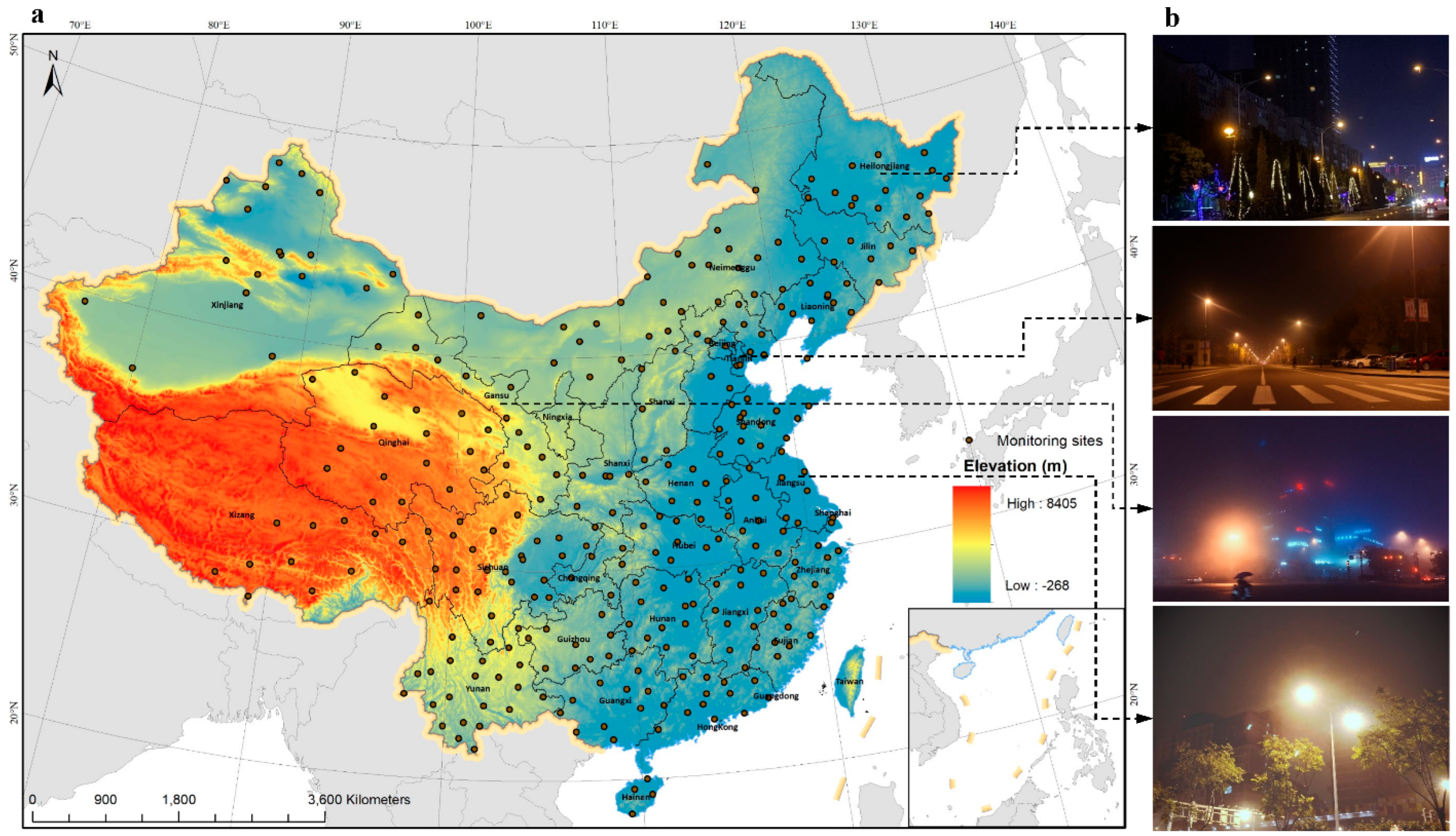
In this experiment, the study area is mainland China (Figure 5), which has various forms of topographical features and meteorological conditions. We obtained the hourly ground-truth visibility data from 319 meteorological monitoring stations in mainland China from June 2018 to May 2019 from the National Center for Environmental Information (NCEI, https://gis.ncdc.noaa.gov/maps/ncei/ (accessed on 25 August 2025)) of the National Oceanic and Atmospheric Administration (NOAA) in the United States. The spatial distribution of these stations is shown in Figure 5a. Hourly visibility data recorded during the nighttime period (defined as 5:00 pm to 12:00 pm and 1:00 am to 5:00 am) were aggregated into daily nighttime averages for evaluating the model’s prediction performance. It should be noted that visibility readings exceeding 30 km were entered as 30 km (a truncated value), and missing values (coded as 999999) were excluded from the analysis. Descriptive statistics of the collected ground-observed visibility are provided in Table 2.
Nighttime smartphone images were collected from the geo-tagged social media platform, Weibo (https://www.weibo.com, accessed on 25 August 2025). We used the crawling technique to obtain images posted by users that included the keyword “night” in Chinese in the post content; the data covered June 2018 to May 2019 from 319 cities in mainland China that correspond to the location of the 319 visibility monitoring stations. Each Weibo record is identified by a unique serial number and contains a set of profile metadata (i.e., username, posting timestamp, posting location, and Weibo post content). We note that nighttime photographs with rain or snow were excluded from the dataset in the pre-processing. The rationale is that precipitation introduces scattering mechanisms that differ fundamentally from those observed in clear, foggy, or hazy conditions [40]. Raindrops and snowflakes are large, non-spherical particles that cause complex visual artifacts such as specular reflections, motion streaks, and irregular diffraction patterns, which cannot be adequately described by standard haze or nighttime haze models [21]. The raw crawled dataset contains 71,289 images, and the pre-processed dataset has 37,052 images remaining. Figure 5b gives examples of these crawled images; Table 2 lists the distribution of these smartphone photographs in various seasons at four geographical zones (i.e., northern China, southern China, northwest China, and Tibet). For model development and evaluation, the dataset was further stratified into training and validation subsets, as described in Section 4.2. This segmentation ensures balanced representation across both geographic regions and seasons.

4.2. Validation of Feature Extraction Framework

4.2.1. Reliability of Separated Glow Layer

Ideally, the evaluation of the separated glow layer is to compare it with a synthetic glow, which is generated by convolving a pre-known light source (i.e., the intensity, shape, and size of the source are given) with a simulated APSF given by ground-truth weather parameters. Although the synthetic glow is an ideal source of data, installing devices for a long period of time to measure in situ weather parameters and light source information for a variety of outdoor scenarios to gather representative samples was considered impractical. However, by visually comparing the separated glow layers and quantitatively analyzing the background layers at similar scenes under varying degrees of haze, we are able to obtain a clear confirmation of the performance of glow layer separation.
Consider an ideal glow layer and background layer decomposed from an observed image, subject to Equation (3), wherein the ideal glow contains only the APSF and light source in the form of Equation (6). Since the multiple scattering of light can be measured by the APSF, there is reason to expect two points: (1) under non-hazy conditions, the background layer should have a high similarity to the observed image except for the light source region; and (2) the shape and intensity of the glow around the light source will be widened and intensified as haze increases, while the background should be constant.
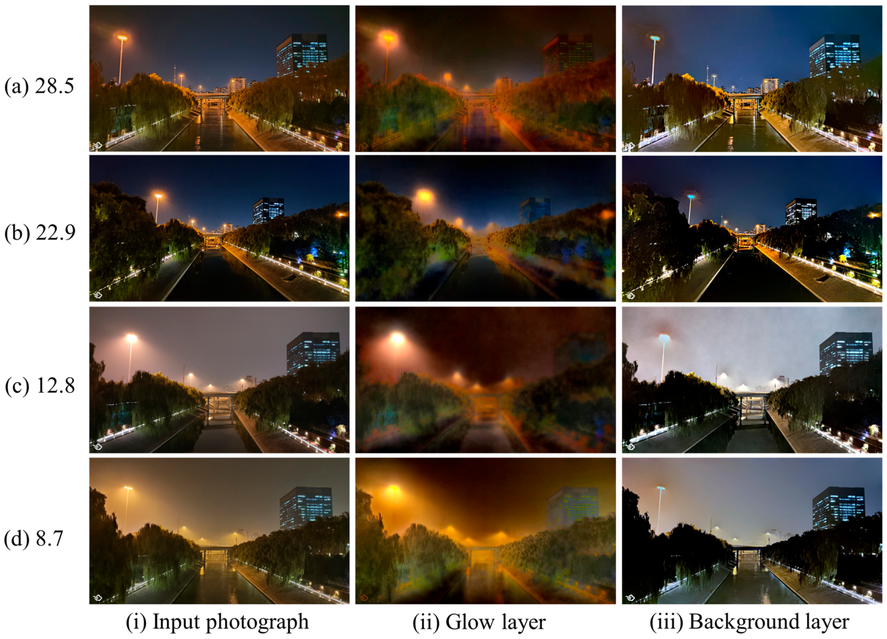
To evaluate the separated glow layer following the above restrictions, photographs taken at the same scenario were selected, and the corresponding layers were compared, as shown in Figure 6. For a clear night (Figure 6a,b), the background layers (Figure 6(a-iii,b-iii)) look very similar to the observed photograph; the differences are mainly at the light sources. This proves that the separation approach correctly captures the necessary information about the presence of haze and does not introduce unwanted information from the background. For the hazy night (Figure 6c,d), the extent of the glow is significantly magnified. This makes evidence that the separation approach has a strong ability in extracting the hazy information under heavy haze conditions. Although we may notice that the glow layers appear to include some background scenes (e.g., trees, rivers, or bridges), we argue that residual information is inevitable for this probability-based approach, as each pixel of the glow layer must have a probability value. In addition, this residual information will be excluded in the forthcoming procedures.
In addition, quantitative analysis of the input photographs and decomposed layers provides another evaluation of the reliability of the layer separation. Following the above restrictions, the background layers should be invariant to varying levels of haze. Two evaluation criteria are used, namely structural similarity index measure (SSIM) and peak signal-to-noise ratio (PSNR), to measure the differences between each pair of observed images and background layers and pairs of background layers. The SSIM index is a measure of image similarity by considering three factors: luminance distortion, contrast distortion, and the loss of correlation, and the PSNR index is given by the error between two images. The values of the SSIM index and PSNR index are in [ 0 ,   1 ] and [ 0 ,   ) , respectively; a greater index value means a higher similarity.
Table 3 gives the index values for each pair of images or layers shown in Figure 6. As expected, the similarity between photographs and the background layers decreases as the haze increases. In addition, the values of the SSIM and those of the PSNR are quite similar. Surprisingly, we found that the pair of background layers under similar haze conditions ( I a and I b at clear nights; I c and I d at hazy nights) and under different haze conditions (e.g., I a and I c ; I b and I d ) have close similarity in terms of the similar SSIM index (0.395 for I a and I d ; 0.431 for I a and I b ) and PSNR value (12.106 for I a and I d ; 11.829 for I a and I b ). Therefore, these results provide a convincing illustration of the reliability of separated glow layers.

4.2.2. Reliability of AGGD Approximation for APSF

In this proposed method, we use the asymmetric generalized Gaussian distribution (AGGD) to fit the APSF. Although fitting a process or pattern by a class of Gaussian is a general approach, and similar studies can be found in other disciplines (e.g., in remote sensing, astronomical studies typically use a Gaussian to fit the PSF profile of night light clusters or galaxies), the robustness and reliability of AGGD as a fitting technique for the extracted APSF needs to be tested.
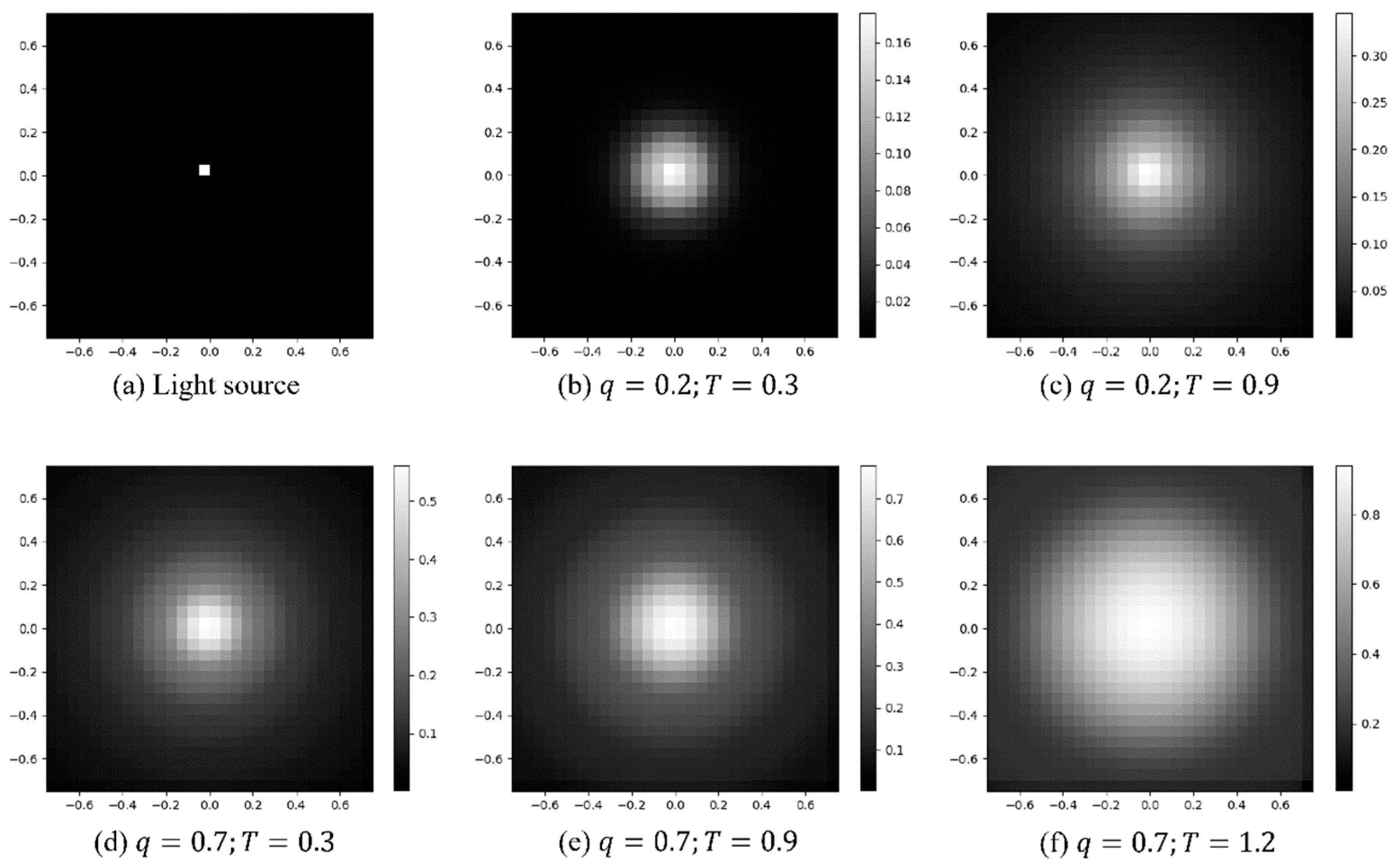
To test the reliability of the AGGD in fitting the projected APSF, we first simulated APSFs, convolved them with a given light source to produce glows, and then projected glows into a two-dimensional plane; the simulation algorithm was the same as that presented in [21,22]. The simulated glows given by different weather parameters are shown in Figure 7. The AGGD was then applied to fit these simulated glows. Table 4 lists the fitted AGGD parameters and a comparison with the simulated parameters. As expected, the fitted results and the simulated parameters are very similar. This consistent and similar pattern reveals the high accuracy of using AGGD to fit glows.
The simulated validation was used to evaluate the performance in an ideal situation (i.e., a centrally symmetrized APSF without any noise). However, the effectiveness of the AGGD fitting approach has not been completely verified, mainly because APSFs extracted from real-world conditions are likely to be of arbitrary shapes. Therefore, the robustness of the fitting method should be further examined. We further compared the performance of AGGD with two widely used distribution functions, namely the generalized Gaussian distribution (GGD) [23] and the two-dimensional standard Gaussian distribution (SGD), in terms of the goodness-of-fit.
Using glows from real-world photographs at different haze levels, we may easily construct the evaluation to examine the robustness of distribution functions. First, we divided the haze levels into five categories (see Table 5). Then, for each category, 20 photographs were selected from our crawled dataset. In the end, three distribution functions (AGGD, GGD, and SGD) were applied to each of these photographs.
The goodness-of-fit values of three distribution functions for each of the four weather categories are recorded in Table 5. The results of AGGD are given in the last line. In general, AGGD is the optimal performance distribution that consistently outperformed the other two distributions in terms of R 2 values. More concretely, the performances of three distribution functions are worse on clear nights (level I) than on hazy nights (level III), of which AGGD is the most preferable. It is noticeable that the value of R 2 increases as haze becomes more severe (level IV).
There are two reasons for the apparent discrepancy. First, for a clear night, the multiple scattering is not dominant, leading to the resultant glow tending to be similar to the light source with respect to different shapes. By introducing the anisotropic parameters, AGGD is less sensitive to outliers and biases so as to yield a significant improvement in fitting the real-world APSFs. In contrast, for the hazy night, the multiple scattering is dominant, and the generated glow tends to exhibit symmetrical concentric rings.

4.3. Performance of Visibility Estimation Model

To examine the applicability of the weather index that was estimated from smartphone photographs for measuring the daily nighttime visibility, the dataset was partitioned into fitting and validation sets. To ensure the data in these two datasets are evenly distributed across space and time, the dataset was first divided into 16 sub-datasets, grouped by four geographical zones (northern China, southern China, northwest China, and Tibet) and four seasons; then, 60% of the data in each sub-dataset was randomly chosen as the fitting data, and the remaining 40% of the data was used for the Hold-out validation (HV).
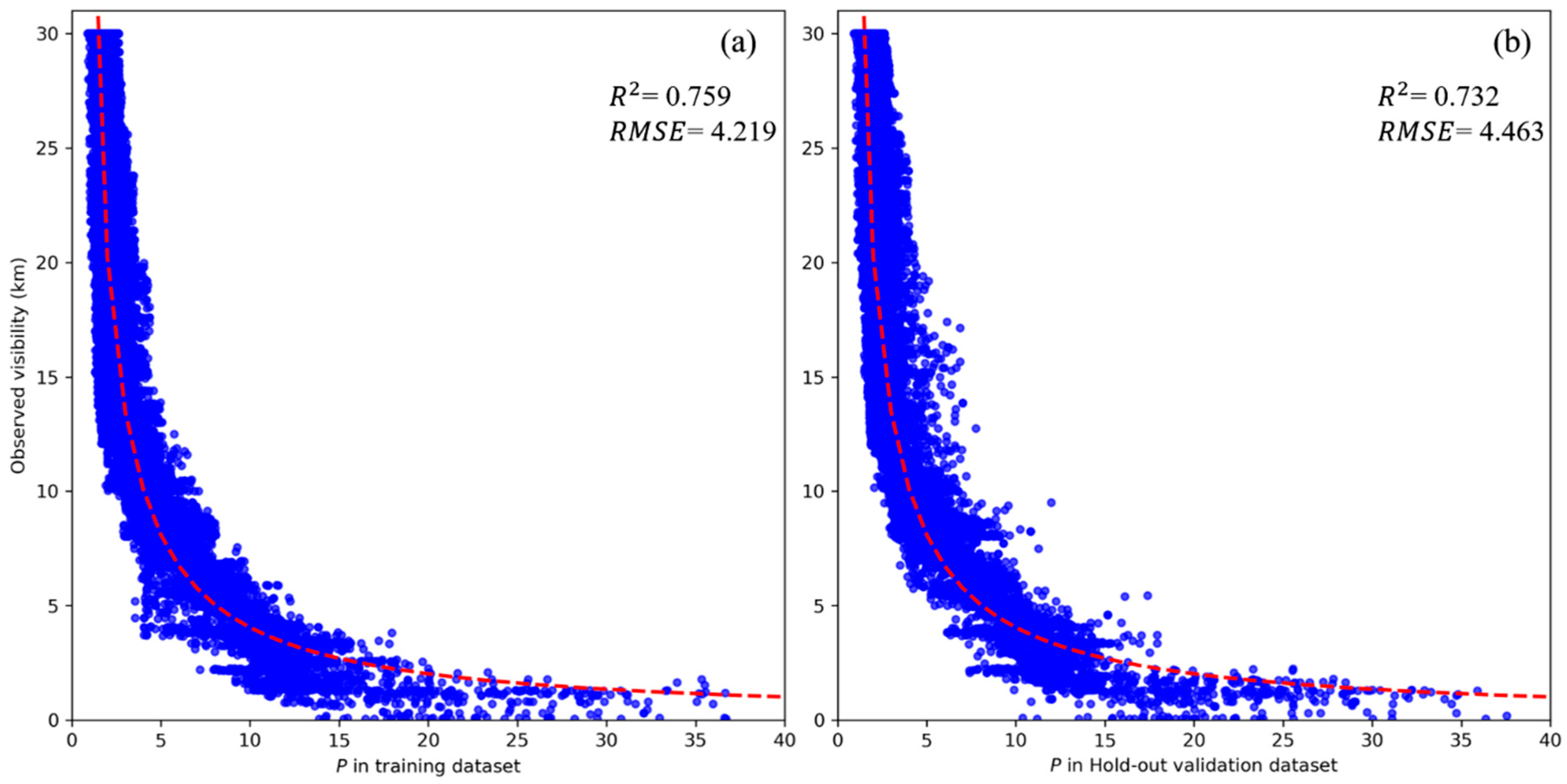
Figure 8 gives model fitting performances between O T I and the nighttime visibility value in fitting and HV datasets. The overall values of goodness-of-fit ( R 2 ) and root-mean-squared error (RMSE) indicate that the model can measure the nighttime visibility with high accuracy (0.759 and 4.219 km in model fitting and 0.732 and 4.463 km in model validation, R 2 , and RMSE, respectively). The model demonstrates consistent performance across the visibility range, including during high (>20 km) and low (<1 km) visibility levels, suggesting its predictive capability throughout diverse scenarios, particularly in the extreme.
To further compare the visibility estimation model’s performances in different geographical zones and four seasons in detail, we summarized the statistics of the results and listed them in Table 3. Generally, the F-statistic values show that this model is statistically significant in different conditions. Performance in each individual case is never below 50% of variation explained and often exceeds 70%, indicating our model is capable in various scenarios. It was found that the average goodness-of-fit value of model fitting and validation in the group of “seasons” (0.740) is higher than that in the group of “geographical zones” (0.702), which shows evidence that the model provides more robust estimates in various seasons than in different geographical zones. The reduced goodness-of-fit value (−0.038) also reveals that the model performances are less affected by seasons but relatively strongly affected by geographic discrepancies. By comparing model fitting performances in four geographical zones listed in Table 3, differences in results suggest that spatial variations are significant. Specifically, we can observe that the best fits were found in northern and southern China (0.783 and 0.771, respectively), with the RMSE value showing a larger difference (RMSE = 4.576 km in northern China vs. RMSE = 3.526 km in southern China). A decreased value of R 2 in the northwest region implies an existing spatial discrepancy (−0.06 to northern China; −0.048 to southern China). In addition, the model performance in Tibet (−0.173 in R 2 and 1.64 km in RMSE, compared to the average fitting performance) also gives a similar pattern and further approves this presented discrepancy. The possible reason for the presence of disparities in estimation performance is that there exists an obvious discrepancy in population density pattern in eastern and western China [41], which made the users’ distribution of the social network platform have an apparent departure and thus led to a deviation of collected data in four geographical zones. For the model validation, performance shows a similar trend where northern China has the best validation result, followed by southern China and the northwest region, whereas Tibet is still the lowest region.
The validity of the model under various seasons is another issue that should be focused on. Generally, Table 6 reveals that the model is robust and valid in four seasons, with temporal variations existing and able to be described by the goodness-of-fit value. The model gives good fits to the data in various seasons except for the summer ( R 2 values in three seasons are above 0.700), with the model fitting best in winter ( R 2 value of 0.826). By comparing the performance in model fitting and HV, the globally decreased R 2 (−0.026) and increased RMSE (0.251 km) indicate that the model has a slight overfit. Similar R 2 values during spring and autumn show that this model fits well and performs robustly in these two seasons. This consistent performance during periods of both potentially unstable (spring) and stable (autumn) weather suggests the model’s ability to handle varying atmospheric conditions. This robustness may also lend support to the underlying assumptions in deriving parameters like the FSI across different seasonal contexts. A possible reason for this is that the summer is the clearest season, while the highest record of visibility is only up to 30 km (see Table 2).
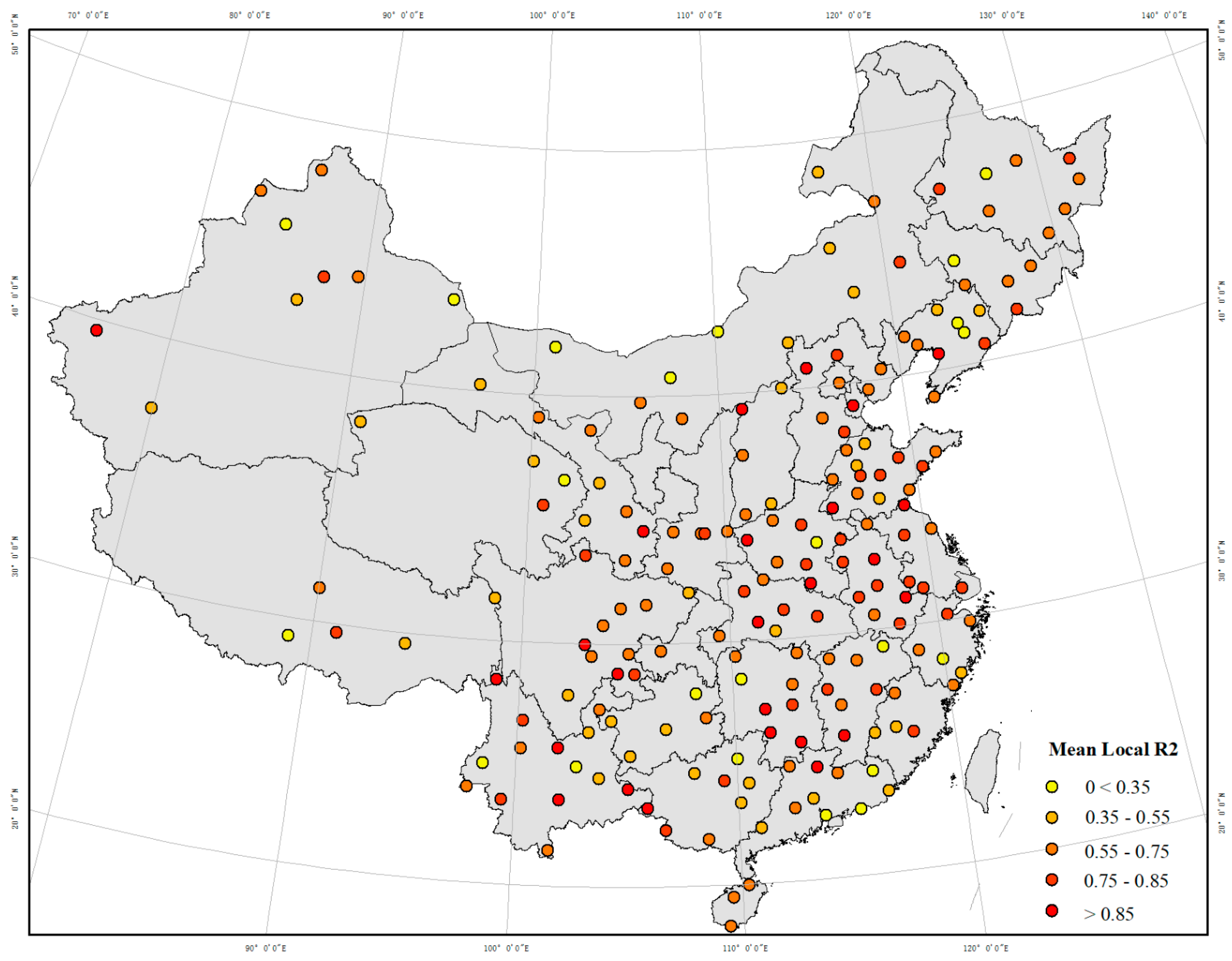
To further explore the spatial heterogeneity in model fitting performances, local R 2 were calculated and are presented in Figure 9. In general, the overall average local R 2 is 0.67, with >25% of the local R 2 are greater than 0.8. Particularly, the spatial distribution of the average local R 2 reveals that the higher R 2 values often correspond to more polluted areas, such as eastern China and urban centers like provincial capitals. Conversely, while overall R 2 might be lower in some parts of western China (e.g., Tibet Autonomous Region, Xinjiang Uyghur Autonomous Region, and Inner Mongolia), specific urban centers within these regions show great disparities and had high local R 2 values, such as Lhasa (0.769), Urumchi (0.827), and Hohhot (0.934). The detailed quantitative analysis demonstrates the model’s capability to handle spatial and temporal variations, allowing for robust estimation of nighttime visibility under diverse conditions.

4.4. Spatial and Temporal Patterns of Predicted Nighttime Visibility over Mainland China

4.4.1. General Spatiotemporal Variation of Estimated Nighttime Visibility

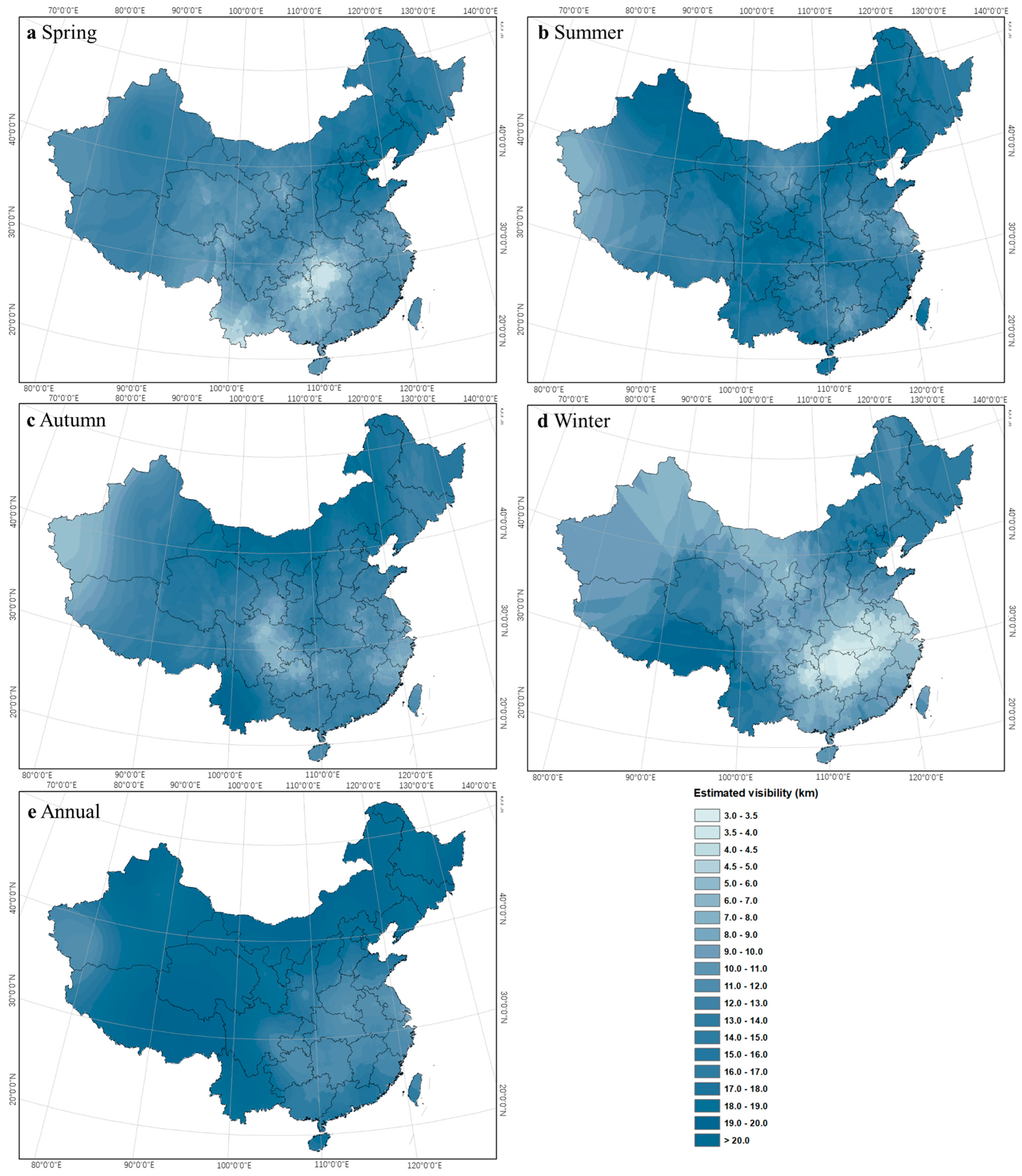
The nighttime visibility was estimated using the collected crowdsourced images, with plots in Figure 10 mapping the resulting seasonally and annually averaged nighttime visibility. To visualize the spatial distribution across mainland China, the ordinary Kriging [42] was employed to interpolate the visibility from station-based to grid-based values. Spatially, the estimated nighttime visibility distribution reveals lower visibility in eastern China, particularly in economically developed areas (e.g., the Yangtze River Delta) and key transportation centers (e.g., Hubei and Hunan provinces), compared to higher visibility in western China. This pattern aligns well with the Hu Huanyong Line [41]. The obviously lowest visibility is particularly presented in central China and the Sichuan Basin, consistent with findings from previous studies [43,44]. Another region of low visibility is observed in the Xinjiang Uyghur Autonomous Region and western Inner Mongolia, located in northwestern China, with the major contributions being the frequent dust events in the Taklamakan Desert [45] and Gobi Desert [46]. Surprisingly, northern China, particularly the Beijing–Tianjin–Hebei (Jinjinji) region (a megacity cluster), exhibited notably higher visibility than southern China. This spatial disparity contrasts with previous findings prior to 2018 [47]. This apparent shift in spatial visibility trends suggests that stringent air pollution regulations implemented after 2013 and 2016 [48] (The Supreme People’s Court, 2016) have contributed to significant improvements in atmospheric visibility in northern and northwest China [49].
Temporally, the seasonal variations are significant in that the nighttime visibility is the most impaired in winter (seasonal mean: 10.46 km) and the clearest in summer (15.25 km). Furthermore, the seasonal variations also have a remarkable disparity, with the variability of visibility being the most prominent in spring and autumn and the least in summer (standard deviation value: 8.047 in spring, 8.027 in autumn, and 7.194 in summer). The seasonal differences are conspicuous in central China and the Sichuan Basin while insignificant in north China. Meanwhile, the noticeable differences in visibility variability also imply that drivers of visibility impairment are sensitive to different geographical areas, local meteorological conditions, and socio-economic factors [44,50,51].

4.4.2. Visibility in Three Hotspots

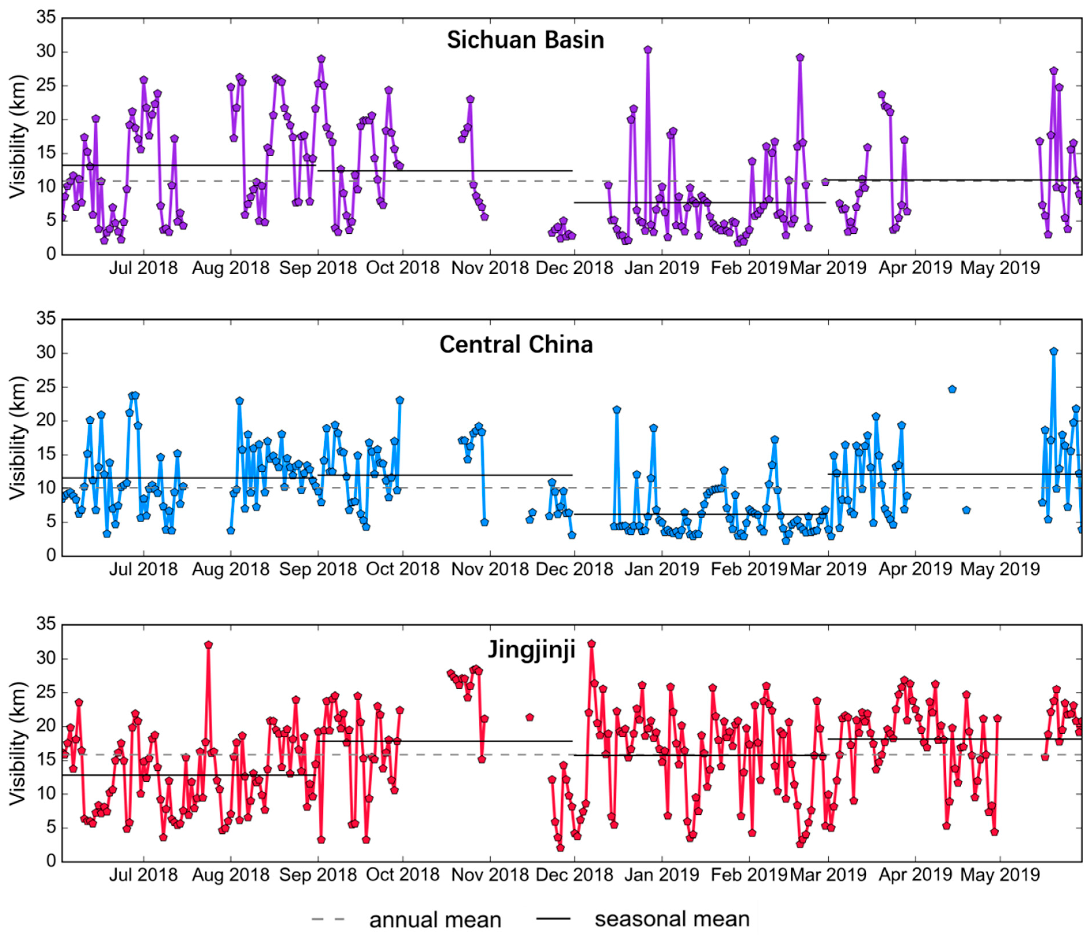
A common issue in visibility estimation models is the uncertainty of their estimates with respect to the diverse conditions in the local region, because the sources of decreased visibility are subject to geographical conditions [52]. Therefore, we focused on three heavily polluted regions with distinct emission characteristics—the Sichuan Basin, central China, and the Jingjinji Metropolitan Region—to analyze daily time-series trends of estimated nighttime visibility (Figure 11) and further assess our model’s sensitivity and applicability. The annual mean nighttime visibility was close between the Sichuan Basin (10.939 km) and central China (10.098 km), but notably higher for the Jinjinji region (15.814 km) (Figure 10e; Figure 11). The temporal variation pattern in the Sichuan Basin was remarkably similar to that of central China, i.e., high in summer and autumn and low in winter. However, this variation pattern was a departure from the Jingjinji region because of the differences in local meteorological conditions.
The Sichuan Basin, a region encompassing Sichuan and Chongqing provinces, exhibited relatively similar nighttime visibility across summer (13.230 km), autumn (12.423 km), and spring (11.087 km). One possible reason for this insignificant seasonal variation is the regions’ propensity for stagnant atmospheric conditions (e.g., low wind speeds and stable relative humidity), which hinder pollutant dispersion [53,54]. Due to the unfavored dispersion conditions, nighttime visibility was most impaired in winter (7.72 km); this deteriorated visibility was particularly low in December and January, while it experienced a slight improvement in February, in agreement with a previous study [55].
Notably, the nighttime visibility experienced extremely poor conditions (3.87 km) during the Chinese Spring Festival period (approximately ranging from 29 January 2019 to 8 February 2019) due to centralized human activities and open-burning events [49,53], suggesting the validity of this proposed nighttime visibility algorithm in extreme severe scenarios. In contrast to winter, visibility significantly improved in summer, potentially due to the joint effect of higher relative humidity and frequent precipitation, which enhance aerosol scavenging [53].
As another polluted, clustered region, central China (i.e., a region covering Hunan and Hubei provinces) has a similar variation pattern in visibility to the Sichuan Basin. The visibility in central China was higher in summer and autumn and decreased sharply from autumn to winter (−5.91 km), with the lowest regions found in mid-February and the end of March (3.773 km; 6.221 km). Frequent clear nights in summer were likely associated with high humidity and strong precipitation, while intense human activity and stagnant meteorological conditions contributed to the deteriorated visibility in central China [49].
The third visibility hotspot, the Jingjinji Metropolitan Region (a Beijing–Tianjin–Hebei region that centered around Beijing), has historically suffered from severe and long-term heavy pollution. Compared to the Sichuan Basin and central China, the Jingjinji region exhibited a higher annual mean nighttime visibility (15.813 km) and an opposite seasonal variability pattern (Figure 11). The superiority of the annual visibility in the Jingjinji region indicates a remarkable improvement in air quality control. Surprisingly, we also found that the observed general improvement trend in visibility from winter to spring was not apparent in Jingjinji, and that winter was no longer the season with the most deteriorating visibility. These observations may be attributed to a series of intensive air pollution prevention and control measures implemented in the Jingjinji region, including the “Action Plan for Prevention and Control of Air Pollution” (2013), the revised “Law on the Prevention and Control of Atmospheric Pollution” (2016), and the establishment of coal-banning zones (by late 2017) [56,57].
Overall, our analysis reveals complex spatiotemporal visibility patterns, with distinct regional characteristics. For instance, while southern China often experienced low visibility in winter, some northern areas like Jinjinji showed different seasonal trends, likely reflecting varying dominant pollution sources and impacts of control measures. The model’s estimation performance (e.g., in terms of agreement with broad trends or ability to capture extremes) was found to be quantitatively robust across these three diverse pollutant regions. This evidence suggests that our proposed algorithm could be applied across diverse spatiotemporal contexts. Importantly, these estimates prove that the proposed algorithm enables a cost-effective way for estimating visibility within a uniform framework. While the experimental results do not imply that this crowdsourced approach (i.e., using smartphone photographs as a low-cost sensor) can replace the conventional measurement methods, our approach can provide valuable supplementary estimates of the ambient environment, particularly in locations or at times lacking conventional ground-truth measurements, thus offering a viable complementary tool for atmospheric sensing.

5. Discussion

In this paper, we have proposed an algorithm using only a single photograph to estimate nighttime visibility. This algorithm first extracts the essential feature that is influenced by multiple scattering at night, i.e., glow effects, from the separated glow layer of the photograph, and thus approximates two weather indices (i.e., optical thickness index [ O T I ] and forward scattering index [ F S I ] ) from the glow by means of the AGGD filter, and then the visibility can be estimated from the weather indices. We conducted experimental validations on a nationwide dataset and evaluated the predictive power of this algorithm using the estimated visibility against ground-truth visibility. The results (Figure 10) demonstrate that the proposed method reliably estimates nighttime visibility levels and reveals spatiotemporal heterogeneity. We also found that the local meteorological conditions and geographical patterns play key roles in visibility variability. Specifically, nighttime visibility tended to be higher (clearer) in the summer and lower (more impaired) in the winter in southern China. In contrast, the opposite pattern was observed in northern China.
By considering the sensitivity of visibility with respect to the diverse conditions in the local regions, we further extended our study on three heavily polluted regions: Sichuan Basin, central China, and Jingjinji Metropolitan Region; presented the time series trends (from June 2018 to May 2019) of nighttime visibility estimated from crowdsourced data (Figure 11); and analyzed the corresponding temporal variations. This regional analysis demonstrates that the visibility estimation model maintained strong prediction accuracy and proved robust for measuring visibility across areas with distinct meteorological conditions. The proposed algorithm offers a reliable nighttime visibility estimation, as reflected by the plausible long-term series trends derived (Figure 11). This capability suggests applicability for various meteorological sensing tasks using smartphone photographs, such as complementing sparse official monitoring networks or assessing localized visibility conditions. These findings reveal that the proposed image processing-based nighttime visibility approach is feasible, holds great potential in predicting nighttime visibility trends, and therefore provides fine-scale spatiotemporal variations.
In addition, our algorithm estimates nighttime estimation relies on only a single smartphone photograph, without any auxiliary information (e.g., pre-defined reference images and pre-known visibility index), which goes beyond the methods used in previous research studies [12]. By relaxing the restrictions on reference data, our algorithm has shown the ability and possibility of single nighttime photographs being used for real-world meteorological monitoring. Furthermore, previous studies have held negative views about applying nighttime photographs in the atmospheric perception, owing to the limitations such as low illuminance, poor quality, or impaired scenes [58] (In contrast to these discussions, the experiments presented in this study provide evidence for the capability of using photographs in monitoring the visibility at night, broaden the potential applications with nighttime images, and highlight potential advantages to the use of mobile phones as an inexpensive and real-time meteorological sensing platform. In addition, the presented algorithm maps the spatio-temporal variations in nighttime visibility distribution, highlights the potential usage of crowd-sensed data to fill in the gap of sparsely distributed meteorological monitoring stations, and provides more portable ways to measure the visibility and sense the personal-level visibility.
Beyond the capability of the proposed algorithm, this paper shows a possible aspect of crowdsourced data to provide a new avenue for meteorological sensing. Crowdsourced data are now widely available and are considered as a potential addition to traditional observations [15]. With the crowdsourced data, the proposed visibility estimation algorithm would be an economical approach compared to these deployed monitoring sites. As we have shown, current photographs crawled from the Internet could be used to provide real-time visibility estimates, such as long-term and large spatial coverage for monitoring. Additionally, because of the enormous amount of potential data available on the web (e.g., social media platforms like the Sina Weibo platform, Twitter, or Facebook), crowdsourcing approaches could be very effective to provide data on a small spatial scale and time granularity. Nevertheless, crowdsourced data and presented results in our study are limited to the city level because of the privacy issue; this is a problem that is relevant to many crowdsourcing endeavors, where crowdsourced observations are intended to discover potential information that may not align with the commercial intent and privacy protections of these social media platforms. Although data availability is a major concern, it does not preclude the use of such data in many studies. For example, to perform a large-coverage and fine-scale meteorological monitoring, smartphone applications or crowdsourced platforms could be deployed coupled with the proposed algorithm.
Although the proposed algorithm provides a potential avenue for monitoring the surrounding atmosphere in a crowdsourced way, it is still perhaps best viewed as an approach to supplement rather than replace the ground-based measures in the context of some limitations and assumptions. First, the proposed algorithm assumes relatively steady atmospheric conditions (e.g., clear air, haze, or fog), where pixel luminance can be modeled as the aggregate effect of scattering by numerous small particles. This assumption does not hold under precipitation (rain, ice, and snow), where scattering is dominated by large, non-spherical particles. Raindrops are individually detectable and often introduce motion streaks, while snow produces even more complex scattering due to its irregular grain shapes. These dynamic effects cannot be adequately captured by standard haze or nighttime haze models. Future work may address these conditions by integrating stereo imagery or auxiliary meteorological data. Second, the geotagged information of crowdsourced data are scarce (only city-level data are available) owing to the data availability and privacy issue. The potential heterogeneities within the city for characterizing the changes on a finer scale might not be presented. If crowdsourced data with precise geotagged information become available in the future, we will be able to make fine-grained observations in space and time. Nevertheless, this study is geared toward providing an alternative method for measuring the visibility in a low-cost manner in near real-time, and its effectiveness proves the validity of this algorithm in providing accurate nighttime visibility estimates. Third, in this work, edge intelligence refers to the use of citizen smartphones as distributed sensors, where images captured and shared online provide real-time atmospheric data from the network edge. Our focus is algorithmic, and while on-device deployment was not tested here, it remains an important direction for future work.
6. Conclusions

In this paper, we have proposed an algorithm using only a single photograph to estimate nighttime visibility. The algorithm extracts the essential feature that is influenced by multiple scattering at night, i.e., glow effects, from the separated glow layer of the photograph, and thus approximates two weather indices (i.e., optical thickness index and forward scattering index) from the glow by means of the AGGD filter, and then the visibility can be estimated from the weather indices. We validated the algorithm on a nationwide dataset by comparing the estimated visibility against ground-truth measurements. Results demonstrate that the proposed algorithm reliably estimates nighttime visibility and generalizes well across diverse spatiotemporal contexts, revealing meaningful visibility patterns. Importantly, our approach enables a cost-effective and scalable estimation approach using only crowdsourced imagery. While this method is not intended to replace conventional instrumentation, it offers valuable supplementary insights—particularly in areas or time periods lacking traditional ground-based monitoring. This work highlights the potential of smartphone photographs as opportunistic sensors for atmospheric visibility sensing.

Supplementary Materials

The following supporting information can be downloaded at: https://www.mdpi.com/article/10.3390/electronics14183642/s1, S1: Runtime measurement; S2: Model performance comparison with other study; S3: Relative distance estimation with object-detection. Table S1: Stage-wise runtime for our dataset; Table S2: Root-mean-squared error and R2 of visibility estimation based on our dataset; Figure S1: Illustration of local light sources. Reference [59] is cited in the Supplementary Materials.

Author Contributions

Conceptualization, C.D. and S.Y.; methodology, C.D.; validation, C.D.; data curation, C.D.; writing—original draft preparation, C.D. and S.Y.; writing—review and editing, C.D. and S.Y.; visualization, C.D.; supervision, S.Y.; funding acquisition, S.Y. All authors have read and agreed to the published version of the manuscript.

Funding

This research was funded by the Hunan Provincial Natural Science Foundation of China, grant number 2025JJ60253. The funder had no role in the study design, data collection and analysis, decision to publish, or preparation of this manuscript.

Data Availability Statement

The data supporting the findings of this study are described in the Section 4.1. Crowdsourced images and the code for this work are available from the corresponding author.

Conflicts of Interest

The authors declare no competing interests.

Abbreviations

The following abbreviations are used in this manuscript:
AGGDasymmetric generalized Gaussian distribution
APSFatmospheric point spread function
OTIoptical thickness index
FSIforward scattering index

References

  1. Norris, J.R.; Allen, R.J.; Evan, A.T.; Zelinka, M.D.; O’Dell, C.W.; Klein, S.A. Evidence for Climate Change in the Satellite Cloud Record. Nature 2016, 536, 72–75. [Google Scholar] [CrossRef] [PubMed]
  2. Singh, A.; Bloss, W.J.; Pope, F.D. 60 Years of UK Visibility Measurements: Impact of Meteorology and Atmospheric Pollutants on Visibility. Atmos. Chem. Phys. 2017, 17, 2085–2101. [Google Scholar] [CrossRef]
  3. Yu, W.; Xu, R.; Ye, T.; Abramson, M.J.; Morawska, L.; Jalaludin, B.; Johnston, F.H.; Henderson, S.B.; Knibbs, L.D.; Morgan, G.G.; et al. Estimates of Global Mortality Burden Associated with Short-Term Exposure to Fine Particulate Matter (PM2·5). Lancet Planet. Health 2024, 8, e146–e155. [Google Scholar] [CrossRef] [PubMed]
  4. Liu, J.; Ren, C.; Huang, X.; Nie, W.; Wang, J.; Sun, P.; Chi, X.; Ding, A. Increased Aerosol Extinction Efficiency Hinders Visibility Improvement in Eastern China. Geophys. Res. Lett. 2020, 47, e2020GL090167. [Google Scholar] [CrossRef]
  5. Mahowald, N.M.; Ballantine, J.A.; Feddema, J.; Ramankutty, N. Global Trends in Visibility: Implications for Dust Sources. Atmos. Chem. Phys. 2007, 7, 3309–3339. [Google Scholar] [CrossRef]
  6. Ting, Y.-C.; Young, L.-H.; Lin, T.-H.; Tsay, S.-C.; Chang, K.-E.; Hsiao, T.-C. Quantifying the Impacts of PM2.5 Constituents and Relative Humidity on Visibility Impairment in a Suburban Area of Eastern Asia Using Long-Term in-Situ Measurements. Sci. Total Environ. 2022, 818, 151759. [Google Scholar] [CrossRef]
  7. Shukla, K.; Aggarwal, S.G. A Technical Overview on Beta-Attenuation Method for the Monitoring of Particulate Matter in Ambient Air. Aerosol Air Qual. Res. 2022, 22, 220195. [Google Scholar] [CrossRef]
  8. Stone, R.G.; Middleton, W.E.K. Visibility in Meteorology: The Theory and Practice of the Measurement of the Visual Range. Geogr. Rev. 1942, 32, 347. [Google Scholar] [CrossRef]
  9. de Meester, J.; Storch, T. Optimized Performance Parameters for Nighttime Multispectral Satellite Imagery to Analyze Lightings in Urban Areas. Sensors 2020, 20, 3313. [Google Scholar] [CrossRef]
  10. Ma, Y.; Zhang, W.; Zhang, L.; Gu, X.; Yu, T. Estimation of Ground-Level PM2.5 Concentration at Night in Beijing-Tianjin-Hebei Region with NPP/VIIRS Day/Night Band. Remote Sens. 2023, 15, 825. [Google Scholar] [CrossRef]
  11. Babari, R.; Hautière, N.; Dumont, É.; Paparoditis, N.; Misener, J. Visibility Monitoring Using Conventional Roadside Cameras—Emerging Applications. Transp. Res. Part C Emerg. Technol. 2012, 22, 17–28. [Google Scholar] [CrossRef]
  12. Gallen, R.; Cord, A.; Hautière, N.; Dumont, É.; Aubert, D. Nighttime Visibility Analysis and Estimation Method in the Presence of Dense Fog. IEEE Trans. Intell. Transp. Syst. 2015, 16, 310–320. [Google Scholar] [CrossRef]
  13. Sakaino, H. PanopticVis: Integrated Panoptic Segmentation for Visibility Estimation at Twilight and Night. In Proceedings of the 2023 IEEE/CVF Conference on Computer Vision and Pattern Recognition Workshops (CVPRW), Vancouver, BC, Canada, 17–24 June 2023; pp. 3385–3398. [Google Scholar]
  14. Kamel Boulos, M.N.; Resch, B.; Crowley, D.N.; Breslin, J.G.; Sohn, G.; Burtner, R.; Pike, W.A.; Jezierski, E.; Chuang, K.-Y.S. Crowdsourcing, Citizen Sensing and Sensor Web Technologies for Public and Environmental Health Surveillance and Crisis Management: Trends, OGC Standards and Application Examples. Int. J. Health Geogr. 2011, 10, 67. [Google Scholar] [CrossRef]
  15. Minson, S.E.; Brooks, B.A.; Glennie, C.L.; Murray, J.R.; Langbein, J.O.; Owen, S.E.; Heaton, T.H.; Iannucci, R.A.; Hauser, D.L. Crowdsourced Earthquake Early Warning. Sci. Adv. 2015, 1, e1500036. [Google Scholar] [CrossRef]
  16. Matthews, M.P. Visibility Estimation Through Image Analytics; Massachusetts Institute of Technology Lincoln Laboratory: Lexington, MA, USA, 2023. [Google Scholar]
  17. Matthews, S.K. From Cell Phone Camera to Satellite Sensor. Trans-Asia Photogr. Rev. 2015, 5. [Google Scholar] [CrossRef]
  18. Mondal, J.J.; Islam, M.F.; Islam, R.; Rhidi, N.K.; Newaz, S.; Manab, M.A.; Islam, A.B.M.A.A.; Noor, J. Uncovering Local Aggregated Air Quality Index with Smartphone Captured Images Leveraging Efficient Deep Convolutional Neural Network. Sci. Rep. 2024, 14, 1627. [Google Scholar] [CrossRef] [PubMed]
  19. Pudasaini, B.; Kanaparthi, M.; Scrimgeour, J.; Banerjee, N.; Mondal, S.; Skufca, J.; Dhaniyala, S. Estimating PM2.5 from Photographs. Atmos. Environ. X 2020, 5, 100063. [Google Scholar] [CrossRef]
  20. Yamasaki, A.; Takauji, H.; Kaneko, S.; Kanade, T.; Ohki, H. Denighting: Enhancement of Nighttime Images for a Surveillance Camera. In Proceedings of the 2008 19th International Conference on Pattern Recognition, Tampa, FL, USA, 8–11 December 2008; pp. 1–4. [Google Scholar]
  21. Narasimhan, S.G.; Nayar, S.K. Contrast Restoration of Weather Degraded Images. IEEE Trans. Pattern Anal. Mach. Intell. 2003, 25, 713–724. [Google Scholar] [CrossRef]
  22. Narasimhan, S.G.; Nayar, S.K. Chromatic Framework for Vision in Bad Weather. In Proceedings of the IEEE Conference on Computer Vision and Pattern Recognition. CVPR 2000 (Cat. No.PR00662), Hilton Head Island, SC, USA, 13–15 June 2000; Volume 1, pp. 598–605. [Google Scholar]
  23. Metari, S.; Deschenes, F. A New Convolution Kernel for Atmospheric Point Spread Function Applied to Computer Vision. In Proceedings of the 2007 IEEE 11th International Conference on Computer Vision, Rio de Janeiro, Brazil, 14–21 October 2007. [Google Scholar]
  24. Fattal, R. Raanan Fattal Single Image Dehazing. ACM Trans. Graph. 2008, 27, 1–9. [Google Scholar] [CrossRef]
  25. Tan, R.T. Visibility in Bad Weather from a Single Image. In Proceedings of the 2008 IEEE Conference on Computer Vision and Pattern Recognition, Anchorage, AK, USA, 23–28 June 2008; pp. 1–8. [Google Scholar]
  26. Jin, Y.; Lin, B.; Yan, W.; Yuan, Y.; Ye, W.; Tan, R.T. Enhancing Visibility in Nighttime Haze Images Using Guided APSF and Gradient Adaptive Convolution. In Proceedings of the 31st ACM International Conference on Multimedia, Ottawa, ON, Canada, 29 October–3 November 2023; pp. 2446–2457. [Google Scholar]
  27. Li, Y.; Tan, R.T.; Brown, M.S. Nighttime Haze Removal with Glow and Multiple Light Colors. In Proceedings of the 2015 IEEE International Conference on Computer Vision (ICCV), Santiago, Chile, 7–13 December 2015; pp. 226–234. [Google Scholar]
  28. Chandrasekhar, S. Radiative Transfer; Courier Corporation: Chelmsford, MA, USA, 1960. [Google Scholar]
  29. Mishchenko, M.I. Multiple Scattering, Radiative Transfer, and Weak Localization in Discrete Random Media: Unified Microphysical Approach. Rev. Geophys. 2008, 46, RG2003. [Google Scholar] [CrossRef]
  30. Henyey, L.G.; Greenstein, J.L. Diffuse Radiation in the Galaxy. Astrophys. J. 1941, 93, 70–83. [Google Scholar] [CrossRef]
  31. Middleton, W.E.K. Vision through the Atmosphere. In Geophysik II/Geophysics II; Bartels, J., Ed.; Springer: Berlin/Heidelberg, Germany, 1957; pp. 254–287. ISBN 978-3-642-45881-1. [Google Scholar]
  32. Nacereddine, N.; Goumeidane, A.B. Asymmetric Generalized Gaussian Distribution Parameters Estimation Based on Maximum Likelihood, Moments and Entropy. In Proceedings of the 2019 IEEE 15th International Conference on Intelligent Computer Communication and Processing (ICCP), Cluj-Napoca, Romania, 5–7 September 2019; pp. 343–350. [Google Scholar]
  33. Li, Y.; Brown, M.S. Single Image Layer Separation Using Relative Smoothness. In Proceedings of the 2014 IEEE Conference on Computer Vision and Pattern Recognition, Columbus, OH, USA, 23–28 June 2014; pp. 2752–2759. [Google Scholar]
  34. Sreejith, S.; Slosar, A.; Wang, H. Point Spread Function Deconvolution Using a Convolutional Autoencoder for Astronomical Applications. arXiv 2024, arXiv:2310.19605. [Google Scholar]
  35. Abrahams, A.; Oram, C.; Lozano-Gracia, N. Deblurring DMSP Nighttime Lights: A New Method Using Gaussian Filters and Frequencies of Illumination. Remote Sens. Environ. 2018, 210, 242–258. [Google Scholar] [CrossRef]
  36. Tesei, A.; Regazzoni, C.S. The Asymmetric Generalized Gaussian Function: A New HOS-Based Model for Generic Noise Pdfs. In Proceedings of the 8th Workshop on Statistical Signal and Array Processing, Corfu, Greece, 24–26 June 1996; pp. 210–213. [Google Scholar]
  37. Potenza, M.A.C.; Sabareesh, K.P.V.; Carpineti, M.; Alaimo, M.D.; Giglio, M. How to Measure the Optical Thickness of Scattering Particles from the Phase Delay of Scattered Waves: Application to Turbid Samples. Phys. Rev. Lett. 2010, 105, 193901. [Google Scholar] [CrossRef]
  38. Natanael, G.; Zet, C.; Fosalau, C. Estimating the Distance to an Object Based on Image Processing. In Proceedings of the 2018 International Conference and Exposition on Electrical And Power Engineering (EPE), Iasi, Romania, 18–19 October 2018; pp. 211–216. [Google Scholar] [CrossRef]
  39. Liu, M.; Bi, J.; Ma, Z. Visibility-Based PM2.5 Concentrations in China: 1957–1964 and 1973–2014. Environ. Sci. Technol. 2017, 51, 13161–13169. [Google Scholar] [CrossRef]
  40. Garg, K.; Nayar, S.K. Vision and Rain. Int. J. Comput. Vis. 2007, 75, 3–27. [Google Scholar] [CrossRef]
  41. Hu, H.Y. The Distribution of Population in China, with Statistics and Maps. Acta Geogr. Sin. 1935, 2, 33–74. [Google Scholar] [CrossRef]
  42. Cressie, N. Spatial Prediction and Ordinary Kriging. Math. Geosci. 1988, 20, 405–421. [Google Scholar] [CrossRef]
  43. Fei, Y.; Fu, D.; Song, Z.; Han, S.; Han, X.; Xia, X. Spatiotemporal Variability of Surface Extinction Coefficient Based on Two-Year Hourly Visibility Data in Mainland China. Atmos. Pollut. Res. 2019, 10, 1944–1952. [Google Scholar] [CrossRef]
  44. Fu, W.; Chen, Z.; Zhu, Z.; Liu, Q.; Qi, J.; Dang, E.; Wang, M.; Dong, J. Long-Term Atmospheric Visibility Trends and Characteristics of 31 Provincial Capital Cities in China during 1957–2016. Atmosphere 2018, 9, 318. [Google Scholar] [CrossRef]
  45. He, Q.; Huang, B. Satellite-Based Mapping of Daily High-Resolution Ground PM2.5 in China via Space-Time Regression Modeling. Remote Sens. Environ. 2018, 206, 72–83. [Google Scholar] [CrossRef]
  46. Tiancheng, L.; Qing-dao-er-ji, R.; Ying, Q. Application of Improved Naive Bayesian-CNN Classification Algorithm in Sandstorm Prediction in Inner Mongolia. Adv. Meteorol. 2019, 2019, 5176576. [Google Scholar] [CrossRef]
  47. Xu, W.; Kuang, Y.; Bian, Y.; Liu, L.; Li, F.; Wang, Y.; Xue, B.; Luo, B.; Huang, S.; Yuan, B.; et al. Current Challenges in Visibility Improvement in Southern China. Environ. Sci. Technol. Lett. 2020, 7, 395–401. [Google Scholar] [CrossRef]
  48. Ministry of Ecology and Environment. The State Council Issues Action Plan on Prevention and Control of Air Pollution Introducing Ten Measures to Improve Air Quality. Available online: https://english.mee.gov.cn/News_service/infocus/201309/t20130924_260707.shtml (accessed on 7 May 2025).
  49. Li, X.; Huang, L.; Li, J.; Shi, Z.; Wang, Y.; Zhang, H.; Ying, Q.; Yu, X.; Liao, H.; Hu, J. Source Contributions to Poor Atmospheric Visibility in China. Resour. Conserv. Recycl. 2019, 143, 167–177. [Google Scholar] [CrossRef]
  50. Deng, X.; Tie, X.; Wu, D.; Zhou, X.; Bi, X.; Tan, H.; Li, F.; Jiang, C. Long-Term Trend of Visibility and Its Characterizations in the Pearl River Delta (PRD) Region, China. Atmos. Environ. 2008, 42, 1424–1435. [Google Scholar] [CrossRef]
  51. Zhao, P.; Zhang, X.; Xu, X.; Zhao, X. Long-Term Visibility Trends and Characteristics in the Region of Beijing, Tianjin, and Hebei, China. Atmos. Res. 2011, 101, 711–718. [Google Scholar] [CrossRef]
  52. Yang, Y.; Liao, H.; Lou, S. Increase in Winter Haze over Eastern China in Recent Decades: Roles of Variations in Meteorological Parameters and Anthropogenic Emissions. J. Geophys. Res. Atmos. 2016, 121, 13050–13065. [Google Scholar] [CrossRef]
  53. Li, Y.-C.; Shu, M.; Ho, S.S.H.; Yu, J.-Z.; Yuan, Z.-B.; Liu, Z.-F.; Wang, X.-X.; Zhao, X.-Q. Effects of Chemical Composition of PM2.5 on Visibility in a Semi-Rural City of Sichuan Basin. Aerosol Air Qual. Res. 2018, 18, 957–968. [Google Scholar] [CrossRef]
  54. Liu, F.; Tan, Q.; Jiang, X.; Yang, F.; Jiang, W. Effects of Relative Humidity and PM2.5 Chemical Compositions on Visibility Impairment in Chengdu, China. J. Environ. Sci. 2019, 86, 15–23. [Google Scholar] [CrossRef] [PubMed]
  55. Zhang, J.; Zhao, P.; Wang, X.; Zhang, J.; Liu, J.; Li, B.; Zhou, Y.; Wang, H. Main Factors Influencing Winter Visibility at the Xinjin Flight College of the Civil Aviation Flight University of China. Adv. Meteorol. 2020, 2020, 8899750. [Google Scholar] [CrossRef]
  56. Liu, G.; Xin, J.; Wang, X.; Si, R.; Ma, Y.; Wen, T.; Zhao, L.; Zhao, D.; Wang, Y.; Gao, W. Impact of the Coal Banning Zone on Visibility in the Beijing-Tianjin-Hebei Region. Sci. Total Environ. 2019, 692, 402–410. [Google Scholar] [CrossRef]
  57. Zhang, Y.; Gao, L.; Cao, L.; Yan, Z.; Wu, Y. Decreasing Atmospheric Visibility Associated with Weakening Winds from 1980 to 2017 over China. Atmos. Environ. 2020, 224, 117314. [Google Scholar] [CrossRef]
  58. Ma, J.; Ma, Y.; Li, C. Infrared and Visible Image Fusion Methods and Applications: A Survey. Inf. Fusion 2019, 45, 153–178. [Google Scholar] [CrossRef]
  59. Su, P.; Liu, Y.; Tarkoma, S.; Rebeiro-Hargrave, A.; Petaja, T.; Kulmala, M.; Pellikka, P. Retrieval of Multiple Atmospheric Environmental Parameters From Images with Deep Learning. IEEE Geosci. Remote Sens. Lett. 2022, 19, 1–5. [Google Scholar] [CrossRef]
Figure 1. Example of smartphone photographs and the process of imaging on a clear night (a) and a hazy night (b).
Electronics 14 03642 g001
Figure 2. Diagram of the proposed algorithm.
Electronics 14 03642 g002
Figure 3. Four examples of nighttime smartphone photographs (ad) from clear mist to heavy haze; glow layers (eh); and de-glow layers (il) from smartphone photos.
Electronics 14 03642 g003
Figure 4. Examples of glow under three weather conditions, glow effects around light sources, and fitted parameters under three different visibility levels. (A) Glow layers of the nighttime hazy images under different visibility levels—high (a), medium (d), and low visibility (g). (B) Iso-brightness contours of the glow effect around light sources showing asymmetric concentric rings—high (b), medium (e), and low visibility (h). (C) APSF fitted by AGGD—high (c), medium (f), and low visibility (i).
Electronics 14 03642 g004
Figure 5. The spatial distribution of visibility monitoring sites, the geography of Weibo posts, and examples of crowdsourced photographs. (a) The spatial distribution of 319 visibility monitoring stations in mainland China. (b) Four examples of web-crawled nighttime smartphone photographs from Weibo (i.e., clear night view, lightly hazy night, medium-hazy night, and heavily hazy night).
Electronics 14 03642 g005
Figure 6. Visual comparisons of the four photographs (i), glow layers (ii), and background layers (iii) at varying haze levels.
Electronics 14 03642 g006
Figure 7. Simulated light source (a) and the generated glows (bf) convolved by APSFs with different weather parameters.
Electronics 14 03642 g007
Figure 8. The performance of the visibility estimation model between the optical thickness index ( O T I ) and the visibility value in the fitting dataset (a) and the Hold-out validation dataset (b). The red-dashed lines are the best-fitted lines for the linear regression model.
Electronics 14 03642 g008
Figure 9. Spatial distribution of the mean local R 2 value of the validation results across mainland China from June 2018 to May 2019.
Electronics 14 03642 g009
Figure 10. The spatial distributions of predicted mean nighttime visibility: (a) spring, (b) summer, (c) autumn, (d) winter, and (e) annual average.
Electronics 14 03642 g010
Figure 11. Time series of estimated nighttime visibility for three pollution hotspot regions. The variations of nighttime visibility in the Sichuan Basin, central China, and the Jingjinji region exhibit different trends. Gaps in the time series represent days with insufficient crowdsourced images and the lack of ground truth. The dashed line represents the annual average visibility, and the solid line represents the annual average visibility values for each season.
Electronics 14 03642 g011
Table 1. The approximate value of the forward scattering parameter q under various weather conditions.
Weather ConditionsClear AirSmall AerosolHazeMist and FogRain
q 0.0–0.20.2–0.70.7–0.80.8–0.90.9–1.0
Table 2. The descriptive statistics of the ground-observed visibility and crowdsourced smartphone photographs.
CategoryGroupMean (km)Std. Dev (km)Min (km)Max (km)Median (km)Count *
Whole14.0268.6020.0530.0012.1437,052
SeasonSpring15.6368.6020.0530.0014.008002
Summer15.8507.5910.0530.0014.129858
Autumn14.6476.3890.1030.0013.007876
Winter10.8658.5550.0530.008.0711,316
Geographical zoneNorthern15.9668.6990.0530.0015.6016,068
Southern11.3177.2340.0530.0010.0017,172
Northwest19.8399.8470.6130.0023.202979
Tibet27.1033.75118.4030.0030.00833
* The number of collected smartphone photographs in each category.
Table 3. The results of the structural similarity index measure (SSIM) and peak signal-to-noise ratio (PSNR) among different pairs of observed photographs and/or background layers I .
SSIMPSNR
Observed I a I b I c I d Observed I a I b I c I d
I a 0.90010.4310.3470.39521.18510011.8299.16412.106
I b 0.7910.43110.3170.31322.16411.8291008.08210.581
I c 0.7650.3470.31710.49614.7029.1648.08210014.691
I d 0.6960.3950.3130.496118.26612.10610.58114.691100
Table 4. Results of the fitted AGGD parameters and simulated parameters.
Glow(b)(c)(d)(e)(f)
Estimated q 0.2100.1980.6950.6970.700
Simulated q 0.20.20.70.70.7
Estimated T 0.3020.9110.2970.8911.195
Simulated T 0.30.90.30.91.2
Table 5. Average goodness-of-fit R 2 values for GGD, SGD, and AGGD for varying visibility levels.
Level of HazeIIIIIIIV
Range (km)(20–30](10–20](5–10] 5
GGD0.7400.8130.8140.856
SGD0.7190.7950.8210.832
AGGD 0.8150.8540.8180.907
For ease of interpretation, the highest R 2 of each haze level is marked in bold.
Table 6. The model fitting performance of the nighttime visibility model in the fitting dataset and Hold-out validation dataset in various geographical zones and four seasons.
CategoryGroup R 2 Value (Fitting)RMSE (km) R 2 Value (HV)RMSE (km)F-Statistic
Geographical zoneNorthern0.7834.5760.7684.8652.261 × 105
Southern0.7713.5260.7473.6522.389 × 105
Northwest0.7235.1380.6905.5444.274 × 104
Tibet0.5296.5990.4977.5373.44 × 101
Average0.7024.9590.6765.398-
SeasonSpring0.7334.4570.7124.7491.140 × 105
Summer0.6574.5560.6204.8301.305 × 105
Autumn0.7424.3540.7164.6121.070 × 105
Winter0.8263.5770.8073.7551.518 × 105
Average0.7404.2360.7144.487-
All0.7594.2190.7324.4635.031 × 105
* Whole dataset--0.7574.3186.171 × 105
* This row represents the RMSE and R 2 value of the linear regression model between ground-truth visibility and estimated visibility.
Disclaimer/Publisher’s Note: The statements, opinions and data contained in all publications are solely those of the individual author(s) and contributor(s) and not of MDPI and/or the editor(s). MDPI and/or the editor(s) disclaim responsibility for any injury to people or property resulting from any ideas, methods, instructions or products referred to in the content.