Article

Ultra-Short-Term Photovoltaic Cluster Power Prediction Based on Photovoltaic Cluster Dynamic Clustering and Spatiotemporal Heterogeneous Dynamic Graph Modeling

1
Key Laboratory of Modern Power System Simulation and Control & Renewable Energy Technology, Ministry of Education, Northeast Electric Power University, Jilin 132012, China
2
School of Computer Science, Baicheng Normal University, Baicheng 137099, China
*
Author to whom correspondence should be addressed.
Electronics 2025, 14(18), 3641; https://doi.org/10.3390/electronics14183641
Submission received: 29 July 2025 / Revised: 5 September 2025 / Accepted: 12 September 2025 / Published: 15 September 2025
(This article belongs to the Special Issue Renewable Energy Power and Artificial Intelligence)

Abstract

Ultra-short-term photovoltaic (PV) cluster power prediction (PCPP) is crucial for intra-day energy dispatch. However, it faces significant challenges due to the chaotic nature of atmospheric systems and errors in meteorological forecasting. To address this, we propose a novel ultra-short-term PCPP strategy that introduces a dynamic smoothing mechanism for PV clusters. This strategy introduces a smoothing convergence function to quantify sequence fluctuations and employs dynamic clustering based on this function to identify PV stations with complementary smoothing effects. We model the similarities in fluctuation amplitude, trend correlation, and degree correlation among sub-cluster nodes using a spatiotemporal heterogeneous dynamic graph convolutional neural network (STHDGCN). Three dynamic heterogeneous graphs are constructed to represent these spatiotemporal evolutionary relationships. Furthermore, a bidirectional temporal convolutional neural network (BITCN) is integrated to capture the temporal dependencies within each sub-cluster, ultimately predicting the output of each node. Experimental results using real-world data demonstrate that the proposed method reduces the normalized root mean square error (NRMSE) and normalized mean absolute error (NMAE) by an average of 6.90% and 4.15%, respectively, while improving the coefficient of determination (R2) by 34.36%, compared to conventional cluster prediction approaches.

1. Introduction

With the continuous advancement of semiconductor and optoelectronic technologies [1,2], the PV industry and its installed capacity have experienced significant year-by-year growth. Ultra-short-term PCPP is indispensable for the refined operation of power systems [3,4,5,6,7,8,9,10], directly supporting intra-day optimal dispatch and rolling generation scheduling. In practice, prevailing technical routes rely on statistical methods [11,12], physical methods [13], and artificial intelligence methods [14,15,16]. Most of these approaches build temporal forecasting models based on historical power data. Due to the limitations of relying solely on historical power data, a large body of research incorporates Numerical Weather Prediction (NWP) information to enhance prediction performance [17,18,19,20]. However, the inherent chaos of weather systems [21,22,23,24], the suddenness and destructiveness of extreme events [25,26,27], and the systematic biases in NWP [28] collectively create a complex and formidable challenge, making breakthrough improvements in ultra-short-term PV prediction accuracy elusive.
In aggregated PV power forecasting, mainstream modeling strategies include the holistic approach [29], the cumulative method, statistical upscaling, and cluster division [30]. The holistic method treats the entire cluster as a single entity, directly predicting the total output using aggregated meteorological data. However, it overlooks local weather variations, which limits its accuracy. The cumulative method forecasts each plant individually and sums the results. It has been used in wind/solar hybrid prediction [31] and with Markov-chain models [32], but often underperforms due to local meteorological interference and error accumulation. Statistical upscaling reduces complexity by selecting representative stations and scaling their outputs proportionally or via parametric relations [33,34,35]. Although computationally efficient, it generally yields lower accuracy because it fails to capture intricate local meteorological effects. In contrast, cluster division classifies stations with similar meteorological or power characteristics into sub-clusters, improving both efficiency and accuracy [36,37,38]. However, static division struggles to adapt to sudden meteorological changes, leading to inconsistent performance over time [39]. Cumulative methods incur high costs and errors that scale with the number of stations. Holistic and statistical upscaling strategies improve efficiency through averaging or representative selection [40] but ignore global meteorology and spatiotemporal correlations, reducing adaptability and accuracy. Static cluster division accounts for power traits and temporal dependencies, yet cannot model time-varying inter-station relationships, resulting in unstable long-term accuracy.
In order to balance prediction accuracy and modeling efficiency, the recent development of multi-node joint modeling with a graph neural network (GNN) provides a powerful technical backbone for PV cluster forecasting. It achieves spatiotemporal fusion and joint modeling of information within a cluster through a single model, like a GNN [41,42,43], graph convolutional network (GCN) [44,45], or graph attention (GAT) network [46,47,48]. Compared with traditional single-node modeling, GNNs integrate inter-node relational information and markedly boost overall accuracy. Consequently, numerous studies have leveraged GNNs to achieve high-precision PV forecasting [49,50,51]. Nevertheless, conventional GNNs focus on information fusion within a single-graph structure [52], extracting features solely through a fixed set of node connections and edge metrics [53,54]. A complete network, however, may exhibit multiple complex relational patterns that collectively describe system evolution. Therefore, recent works have shifted from a single-graph paradigm to heterogeneous graph structures for more flexible forecasting [55,56]. By jointly exploiting several graphs with distinct connectivity relations, heterogeneous graphs extract richer relational information and have been shown to alleviate the information-fusion deficiencies inherent in single-graph models [57,58]. Yet PV forecasting systems evolve dynamically, and static graph strategies inevitably fail to capture variability induced by local factors and may even lead to prediction collapse. Consequently, research has transitioned from static to dynamic graphs to accommodate real-time uncertainty [15,54]. However, current modeling methods based on graph neural networks, while achieving efficient predictions and high-precision modeling of multiple PV power nodes through multi-source information integration strategies, typically model PV clusters using static graph methods. This approach fails to capture the dynamic spatiotemporal evolution relationships of PV power nodes, thereby being unable to further describe the dynamic spatiotemporal evolution patterns of the PV cluster, and the structure type of the graph is simple and has difficulty describing multi-level relationships [59,60,61]. Additionally, almost no studies have combined heterogeneous graphs with dynamic construction for power forecasting with multi-node methods. Ideally, such integration would further enhance PV forecasting accuracy.
In summary, current PV cluster power forecasting primarily relies on the holistic approach, cumulative method, statistical upscaling, and cluster static division paradigms. These methods exhibit high modeling cost, low information utilization, difficulty (or impossibility) in selecting representative plants, and an inability of static feature extraction to track system dynamics. Although GNNs mitigate many of these issues, their predictive gains remain limited by static graph structures and single-connectivity assumptions, which fail to capture the dynamic spatiotemporal evolution relationships of PV power nodes, thereby being unable to further describe the dynamic spatiotemporal evolution patterns of the PV cluster. Heterogeneous graphs capture multiple relational patterns, yet static heterogeneous graphs still fail to track dynamic evolution. To address these gaps, this paper proposes a dynamic cluster division scheme based on smooth convergence and coupled with a spatiotemporal heterogeneous dynamic graph convolutional network to model time-varying PV cluster power. The key contributions are as follows:
(1)
We introduce a function to measure PV power convergence volatility and propose a dynamic clustering method based on volatility smoothing to extract the most predictable component of the PV cluster power.
(2)
We construct three heterogeneous graphs—volatility similarity, trend correlation, and amplitude matching—among sub-clusters to represent the system’s multi-layer relational structure, and we develop a spatiotemporal heterogeneous dynamic graph convolutional network to mine multiple relational patterns during system evolution and model dynamic sub-cluster nodes for effective forecasting of PV cluster power.
(3)
We embed a bidirectional temporal convolutional neural network that accounts for bidirectional temporal dependencies to capture node-level sequential relationships and obtain high-precision predicted PV cluster power.
The remainder of this paper is as follows: Section 2 presents the methodology, Section 3 provides case studies, Section 4 offers analysis and discussion, and Section 5 concludes the paper.

2. Methodology

Across large-scale PV clusters, meteorological characteristics differ markedly from plant to plant. Forecasting strategies that rely on the holistic approach, cumulative method, statistical upscaling, and cluster static divisions therefore struggle to deliver accurate predictions. To accommodate the evolving power output of PV clusters, this paper proposes a dynamic modeling framework that explicitly incorporates system-wide volatility smoothing and multiple spatiotemporal heterogeneous graphs. Firstly, we construct a volatility evaluation function based on sample entropy to quantify the smoothing effect embedded in PV cluster power. This metric is then embedded into a k-means clustering model to enable real-time, dynamic clustering of the PV cluster—identifying sub-clusters whose aggregate output can be smoothed through appropriate power superposition. Second, we deploy multiple heterogeneous graphs within a spatiotemporal heterogeneous dynamic graph convolutional network to capture power fluctuation similarity among sub-clusters and establish an effective dynamic heterogeneous relationship—extracting and fusing multi-relational, dynamic heterogeneous information. Finally, the fused information is fed into a bidirectional temporal convolutional neural network to extract temporal dependency features and predict the output for each node, thereby achieving robust modeling.

2.1. Dynamic Clustering of PV Stations via Aggregation-Smoothing Distance

Across an entire PV cluster, both the magnitude and the direction of power fluctuations vary significantly across plants and across time. Nevertheless, the judicious aggregation of selected plants can markedly attenuate the volatility of the original power sequences and yield a smoother composite signal. In many cases, this aggregated signal exhibits substantially higher predictability. Figure 1 illustrates how sequences of differing volatility combine to produce aggregates with distinct trends and magnitudes. When sequences share similar fluctuation trends, their superposition amplifies volatility (Figure 1c,d). Conversely, when trends oppose one another, the aggregate volatility drops sharply. If the opposing trends are equal in magnitude, the result is a flat line (Figure 1a,b). Superposing a volatile sequence onto a smooth one merely increases the aggregate volatility relative to the smooth input (Figure 1e,f). Thus, if an appropriate grouping strategy reduces volatility after aggregation, as in Figure 1a,b, the resulting sequence becomes markedly more predictable.
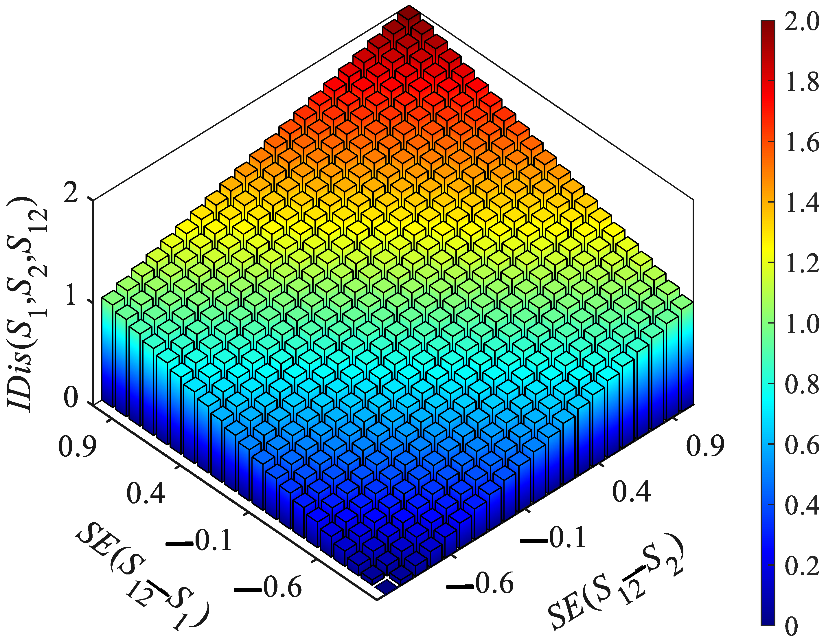
To cluster PV plants that collectively deliver such a volatility-smoothing effect—and thereby enhance predictability—we introduce an improved clustering distance based on sample entropy and embed it within a k-means framework. This distance enables dynamic division of PV plants whose joint output exhibits volatility suppression. The modified clustering distance is defined as follows:
I D i s S 1 , S 2 , S 12 = 1 + S E ( S 12 ) S E ( S 1 ) + 1 + S E ( S 12 ) S E ( S 2 ) 2
where S 1 and S 2 denote the two sequences used for distance assessment, respectively, S 12 denotes the superimposed power sequence, and I D i s denotes the improved clustering distance, whose smaller value indicates that the two sequences fluctuate more similarly. S E ( ) denotes the sample entropy, which is expressed as follows:
S E = ln A m r / B m r
A m r = 1 N m i = 1 N m A i N m 1
B m r = 1 N m i = 1 N m B i N m 1
where N denotes the length of the original sequence used to evaluate the entropy of the sample, m denotes the dimension of the reconstructed feature, r denotes the similarity tolerance threshold, B is the probability of finding a similar pattern (or vector) at the scale of m points, and A is the conditional probability that the m + 1st point is also similar, given that the first m points are similar.
As shown in Figure 2, the improved loss function has significant fluctuation-smoothing properties. When the sample entropy of the superimposed power sequence S 12 is lower than that of the sequences S 1 and S 2 before the superposition, S E ( S 12 ) S E ( S 1 ) as well as S E ( S 12 ) S E ( S 2 ) will exhibit negative values, at which time the corresponding clustering loss is the lowest. In other words, when the sample entropy of a single sequence is greater than S 12 , the superposition of power will produce a convergence-smoothing effect, and, the larger the difference, the more obvious the superposition effect. In contrast, when the sample entropy of the individual sequences is less than S 12 , the superposition of sequences exhibits high volatility because this increases the sample entropy strength. For example, the scenario in Figure 2, where S E ( S 12 ) S E ( S 1 ) as well as S E ( S 12 ) S E ( S 2 ) are both greater than 0 and close to 1, appears to have the largest I D i s S 1 , S 2 , S 12 , which corresponds to the smallest clustering loss value. Replacing this improved loss with the original Euclidean clustering distance of k-means and using it for dynamic clustering of PV sites will effectively extract PV sub-clusters with fluctuation-smoothing effects.

2.2. Spatiotemporal Heterogeneous Dynamic Graph Convolutional Neural Network

Power fluctuation characteristics not only exhibit variability between individual power stations but also differ across sub-clusters formed through dynamic clustering. Exploiting these inter-plant or inter-sub-cluster similarities in fluctuation evolution is therefore pivotal for improving forecasting accuracy. To this end, we introduce a STHDGCN that explicitly models such similarities within PV clusters. STHDGCN is an advanced extension of both heterogeneous graph architectures and graph convolutional networks. Conventional graph convolutional networks enable joint modeling of multiple nodes, yet they neither accommodate heterogeneous connectivity patterns nor capture evolving graph features. Conversely, traditional heterogeneous graphs lack spatiotemporal modeling capacity, which limits their performance. Integrating spatiotemporal heterogeneous graphs with dynamic graph convolution substantially mitigates the accuracy ceiling imposed by insufficient feature fusion and absent temporal dynamics [62,63,64].
(1) Spatiotemporal dynamic heterogeneous graph modeling: Let the sequence of spatiotemporal graphs be G = G t t = 1 T , where G t = V t , ε t , R t , A t , V t denotes the set of nodes (containing K types, ϕ(v):VtA), ε t denotes the set of edges (containing M types, ψ(e):EtR), A t denotes the adjacency tensor (dynamics), and A t R V t × V t × R . In order to efficiently extract the spatiotemporal heterogeneous evolutionary relationships among the PV sub-cluster nodes and capture these heterogeneous dynamic features effectively, three heterogeneous graph structures are introduced on the basis of the dynamics graphs, which are as follows: fluctuating trend correlation heterogeneous graph V t T , fluctuation degree correlation heterogeneous graph V t D , and fluctuation amplitude correlation heterogeneous graph V t A , whose expressions are as follows:
V t T = v T 11 v T 12 v T 1 L v T 21 v T 22 v T 2 L v T M 1 v T M 2 v T M L M × L
V t D = v D 11 v D 12 v D 1 L v D 21 v D 22 v D 2 L v D M 1 v D M 2 v D M L M × L
V t A = v A 11 v A 12 v A 1 L v A 21 v A 22 v A 2 L v A M 1 v A M 2 v A M L M × L
where v T M L , v D M L , and v M M L denote the trend correlation weight, fluctuation degree correlation weight, and fluctuation magnitude correlation weight between the Mth PV sub-cluster node and the Lth sub-cluster node, respectively. Thus, the dynamic heterogeneous graph can be expressed as follows:
V t = V t T , V t D , V t A ,    V t T , V t D , V t A R M × L
where M and L denote the number of target stations and the number of reference neighboring stations, respectively. And the feature vector of target node V i at moment t can be expressed as follows:
V i = V i T , V i D , V i A ,    V i T , V i D , V i A R 1 × L
where the dimension of V i depends on its type ϕ(i), and the dynamic properties are captured through the adjacency matrix A t r (type rR) and the node identity matrix Xt.
(2) Heterogeneous spatiotemporal convolution module: This includes a two-layer structure of a heterogeneous spatial convolution layer (aggregating heterogeneous neighbor information and preserving node type characteristics [65,66,67,68]) and dynamic temporal convolution layer (capturing the temporal evolution of node characteristics and adapting to the dynamic topology), etc. In the part of the heterogeneous spatial convolution layer, it contains three steps to achieve the fusion of heterogeneous neighbor information:
Step 1: Feature Projection (Uniform Dimension): Design the projection matrix W ϕ i R d × d ϕ i for node type ϕ(i) as follows:
z i t = W ϕ i V i t R d
Step 2: Heterogeneous Attention Mechanism: For an edge type rR, compute the attention coefficient of the node j to i as follows:
α i j t , r = exp σ α r T z i t | | z j t | | e i j t k N i r exp σ α r T z i t | | z k t | | e i k t
where e i j t denotes the feature vector of edge i , j , N i r denotes the set of neighbors of node i under relation j, | | denotes vector splicing, and σ denotes the “LeakyReLU” activation function.
Step 3: Multi-Head Aggregation: P attention headers are used in the aggregation process as follows:
h i t , s p a = || p = 1 P r R j N i r α i j t , r , p z j t
In the dynamic temporal convolutional layer part, the gated recurrent unit (GRU) variant is used as follows:
u i t = σ W u h i t , s p a + U u h i t 1 + b u
r i t = σ W r h i t , s p a + U r h i t 1 + b r
h ˜ i t = tanh W r h i t , s p a + U h r i t × h i t 1 + b h
h i t = tanh 1 u i t × h i t 1 + u i t × h ˜ i t
where the input to this part is the output h i t , s p a of the spatial convolution, and the hidden state h i t implicitly fuses the topological dynamics (due to h i t , s p a depending on A t ).
(3) Spatiotemporal feature fusion and prediction: This segment contains three important steps:
Step 1: Graph-level feature dimensionality reduction: Compress the node feature H t = h i t i = 1 V t into a graph-level vector as follows:
s t = M L P R E A D O U T H t ,    1 V t i = 1 V t h i t
Step 2: Timing feature integration: Input s t m , , s t into the timing pooling layer.
O = T e m p o r a l P o o l i n g s t m , , s t
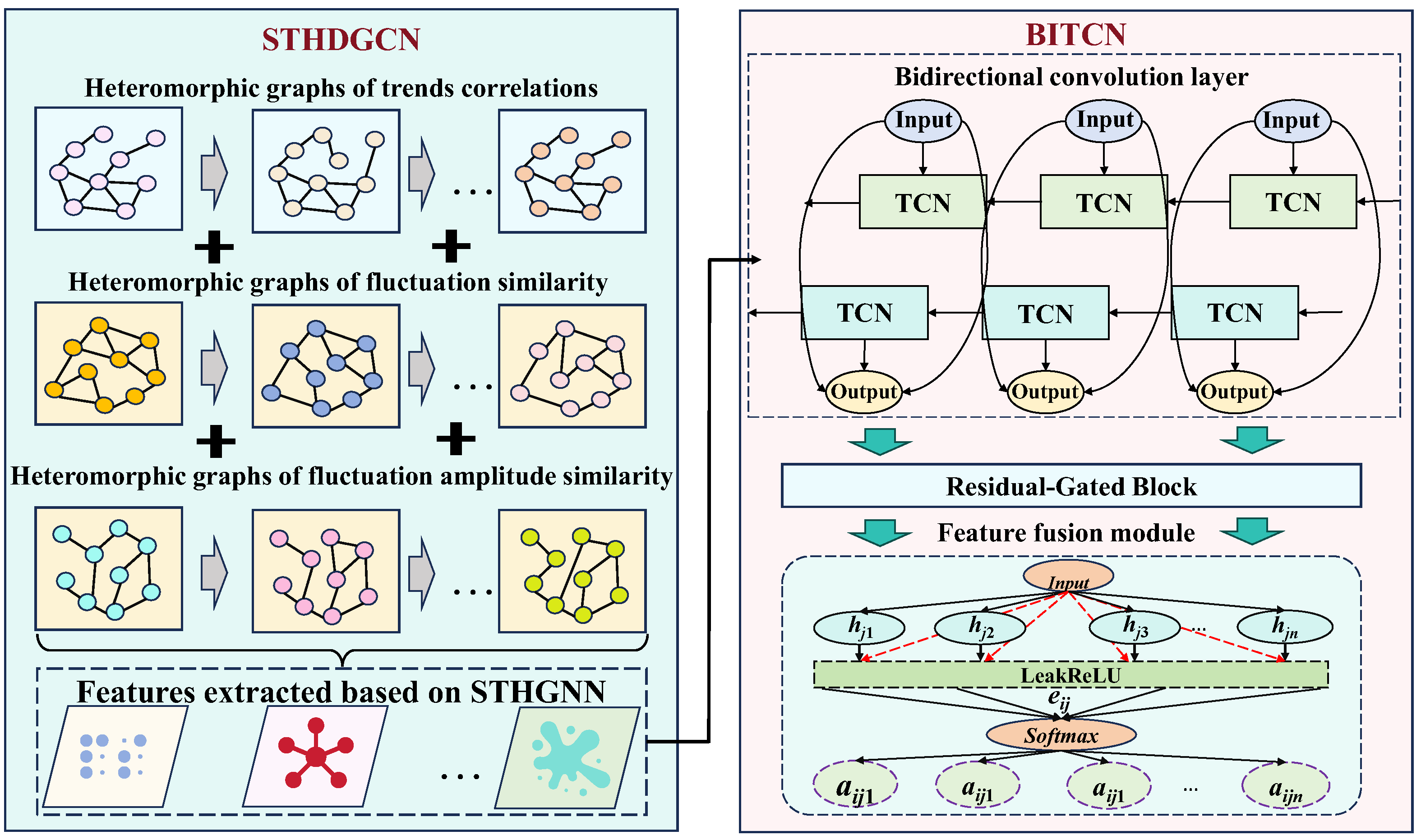
Step 3: In order to effectively extract the timing dependencies of each node, this paper introduces a bidirectional temporal convolutional neural network (BITCN) to describe the evolution process of time-dependent information between nodes and to improve the performance of timing prediction. BITCN, as an improved version of the temporal convolutional neural network (TCN), has a bidirectional timing memory characteristic and is able to deduce the timing lag effect of the input data based on its evolution relationship. The single-layer BITCN architecture comprises two TCN modules [69], which included three modules: the bidirectional convolution layer, Residual-Gated Block, and feature fusion module:
(1) Bidirectional convolution layer: This contains the following forward convolutional paths and backward convolutional paths:
H l t = σ i = 0 K 1 W l i X t d l i + b l , t d l i t
H l t = σ i = 0 K 1 W l i X t d l i + b l , X t = X l , t < l X T , t > T
where W l i and W l i denote the forward and backward weights of the ith convolutional kernel in layer l, b l and b l denote the forward and backward path biases, respectively, d l denotes the expansion factor, and σ denotes the activation function.
(2) Residual-Gated Block: This contains the following gated convolutional units and residual connections:
Z l t = tanh W f t H l 1 t × σ W g l H l 1 t
H l t = ϕ Z l t + F H l 1 t , F H = W r e s H , dim H 0 H , o t h e r w i s e
where W f t denotes feature transformation weights, W g l denotes gating weights, × denotes the Hadamard product, and W r e s denotes 1 × 1 convolution weights.
(3) Feature fusion module: This includes bidirectional feature splicing and attention-weighted fusion as follows:
H b i t = [ H N t ; H N T t + 1 ] R 2 D
Y = t = 1 T α t W o u t H b i t
α t = exp e t τ = 1 T exp e t
e t = v T tanh W a t t n H b i t
where “;” denotes the dimensional splicing operation, T t + 1 is used for temporal alignment, W a t t n denotes the attentional hidden layer weights, v T denotes the attentional score vector, and W o u t denotes the output vector. Figure 3 shows the network architecture of STHDGCN-BITCN.
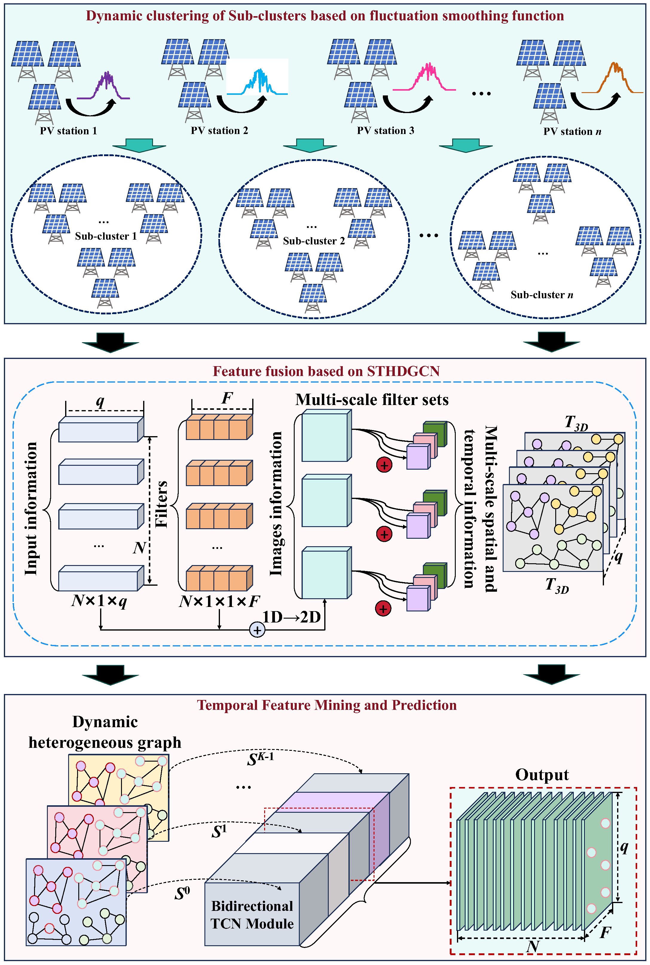
Figure 4 shows the principal technical workflow of this study, which proceeds in three sequential stages:
(1) Dynamic division of the PV cluster via an improved volatility-smoothing function: Prior to forecasting, historical power sequences from every PV plant are extracted and fed into the enhanced clustering loss. Guided by the volatility-smoothing metric, the k-means model assigns plants to distinct sub-clusters. Each resulting sub-cluster contains stations whose joint output yields pronounced smoothing after aggregation, thereby elevating PV cluster predictability.
(2) Spatiotemporal feature extraction and fusion through the heterogeneous dynamic graph convolutional network: The cluster comprises plants whose fluctuations differ in trend, magnitude, and amplitude; these similarities constitute informative priors for describing sub-cluster evolution. Three heterogeneous adjacency matrices within the spatiotemporal graph jointly encode the fluctuation relationships among sub-clusters. The STHDGCN explicitly accounts for spatiotemporal evolution, allowing the three heterogeneous graphs to evolve over time and capture dynamic dependencies, ultimately yielding enriched and dynamically fused representations.
(3) Bidirectional temporal dependency extraction via a BITCN: After STHDGCN delivers spatiotemporal features, each sub-cluster’s sequence is processed by a BITCN to capture forward and backward temporal dependencies, accurately portraying nodal power evolution and enhancing the forecasting accuracy of ultra-short-term PV cluster power.

3. Case Study

To verify the efficacy of the proposed method, we conduct a case study on a PV cluster located in Gansu, China, using data spanning 2020–2022. The model is trained on the continuous two-year dataset from 2020 to 2021, and its performance is validated against the complete 2022 dataset. Input data comprise gridded NWP fields and the measured PV cluster’s historical power. The NWP grid has a spatial resolution of 3 km × 3 km, while both the cluster power and the NWP variables are sampled at 15 min intervals. Among them, the surface dimensions of a single PV panel are 2094 mm × 1038 mm, and the rated power of each PV panel is 250 W. On average, each PV power station has 4000 PV panels, with a total PV panel area of 9000 m2. The rated capacity of the entire cluster is 1 500 MW. The geographical location information of the PV cluster is shown in Table 1. Among them, all the experiments in this paper are completed on the platform of Pycharm 2022. The computer used is configured with a memory capacity of 8.00 GB. It has a Windows 11 ×64 operating system; the processor and graphics card models are AMD Ryzen 5 5600H with Radeon Graphics 3.30 GHz and NVIDIA GeForce RTX 3050 Laptop GPU 4 GB, respectively.
Prediction accuracy is assessed using normalized root mean square error (NRMSE), normalized mean absolute error (NMAE), and the coefficient of determination (R2). The corresponding formulations are given below:
N R M S E =   1 / k i = 1 k p i p i / C a p 2
N M A E = 1 / k i = 1 k p i p i / C a p
R 2 = i = 1 k p i p ¯ 2 i = 1 k p i p i 2 / i = 1 k p i p ¯ 2
where p i represents the ith actual value, p i represents the ith predicted value, p i ¯ represents the mean of the real value, k represents the sequence length, and C a p represents the total installed capacity of the PV cluster.

3.1. Comparison of Prediction Scenarios and Baseline Model

To benchmark the effectiveness of the proposed framework, we compare it—at the cluster modeling level—with a conventional holistic approach, cumulative method, statistical upscaling, and cluster static division approaches [70]. Specifically, the following ablation experiments are designed:
(1)
We apply the traditional holistic approach, cumulative method, statistical upscaling, and cluster static division strategies to forecast PV cluster power and evaluate their prediction performance and accuracy.
(2)
We compare the conventional dynamic cluster division schemes that rely on correlation or volatility metrics with the proposed clustering method based on the volatility-smoothing function under identical model backbones.
(3)
We benchmark the predictive accuracy of (i) conventional static/dynamic graph convolutional networks (SGCN/DGCN), (ii) spatiotemporal heterogeneous static/dynamic graph convolutional networks (STHSGCN/STHDGCN), and (iii) the proposed STHSGCN/STHDGCN coupled with a BITCN (STHSGCN-BITCN/STHDGCN-BITCN) across alternative division schemes.
Each experiment also adopts both single-node and multi-node baselines, including multiple linear regression (MLR), back-propagation neural networks (BP), random forests (RF), BITCN [71,72,73], and Transformer, together with the graph-based variants mentioned above [74].

3.2. Case Study of Traditional Cluster Power Prediction Methods

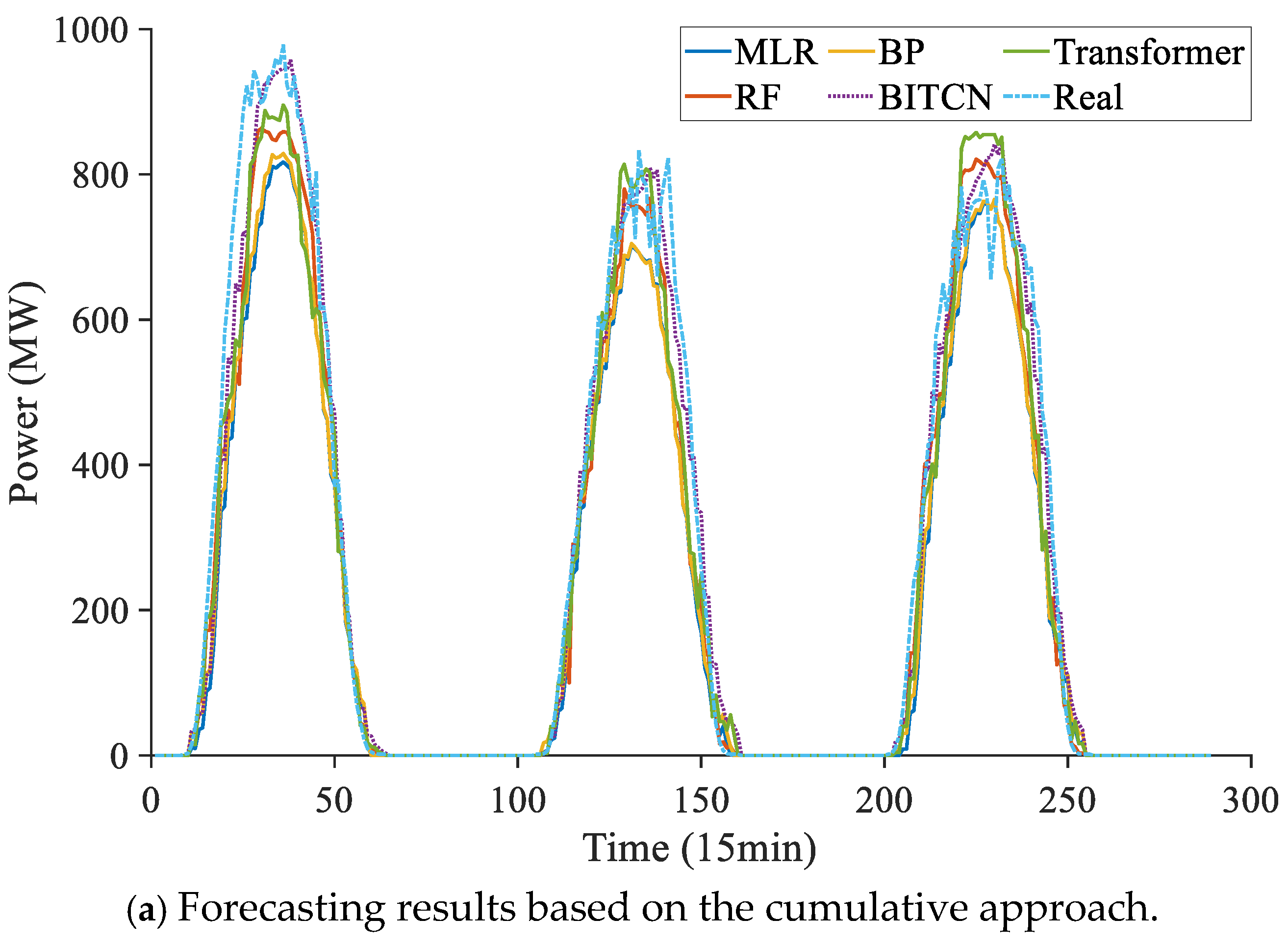
Ablation experiment (1) contrasts the single-node baselines under the four classical cluster modeling strategies. We evaluate MLR, BP, RF, BITCN, and Transformer. All models exhibit markedly different accuracies across strategies; the comparison results are shown in Table 2. Cumulative method forecasts every plant individually and aggregates the results, and error accumulation is inevitable, so accuracy is consistently the lowest. Relative to the cumulative method, the holistic approach reduces NRMSE and NMAE by 0.89% and 0.52% on average, while R2 improves by 9.45%. Statistical upscaling selects representative plants, scales their predictions by a statistical ratio, and approximates cluster output. Because meteorological evolution across the cluster is non-uniform, local meteorology seldom mirrors cluster behavior, and representative plants cannot track the power of PV clusters in real time. Consequently, statistical upscaling yields the worst accuracy: NRMSE and NMAE exceed those of the holistic approach and cumulative method by 1.26% and 0.77%, respectively, while R2 drops by 20.08%. To capture local characteristics, many studies adopt static cluster division. This strategy outperforms the other three: NRMSE and NMAE fall by 1.47% and 0.82% relative to the best competitor, and R2 rises by 17.17%. Thus, among traditional schemes, static cluster division is the most accurate, whereas statistical upscaling is the least. Figure 5 displays three-day continuous forecast traces for each modeling strategy. MLR, RF, and BP show limited learning capacity and consistently underestimate power. Deep-learning models—especially BITCN—track the temporal evolution accurately, yielding curves that closely follow the ground truth.

3.3. Comparative Analysis of Predictive Performance Across Different Dynamic Clustering Methods

For the ablation experiment (2), this part mainly compares the differences and modeling performance of the different cluster division bases in the cluster dynamic division mechanism with the division method corresponding to the fluctuation-smoothing effect indicator proposed in this paper. In the comparative division mechanism, the trend correlation based on the correlation coefficient and the similarity based on fluctuation are mainly used to divide the clusters, and the division mechanism is as follows:
R S , S = i = 1 n S i S ¯ S i S ¯ i = 1 n S i S ¯ 2 i = 1 n S i S ¯ 2
D S e S , S = S E S S E S
where R denotes the correlation coefficient corresponding to the sub-cluster power sequences S as well as S . If the correlation coefficient of the two sequences is larger, the two sub-clusters need to be classified as the same type, while D s e denotes the sample entropy difference corresponding to the sequences S as well as S , which indicates the similarity of the degree of fluctuation of the two sequences. If the entropy difference of the two sequences is lower, it means that their fluctuations are more similar. By incorporating these two similarity formulas into the k-means clustering model for screening PV sub-clusters with similar evolutionary trends and similar fluctuations, we can realize the dynamic division of PV clusters based on different criteria [75,76].
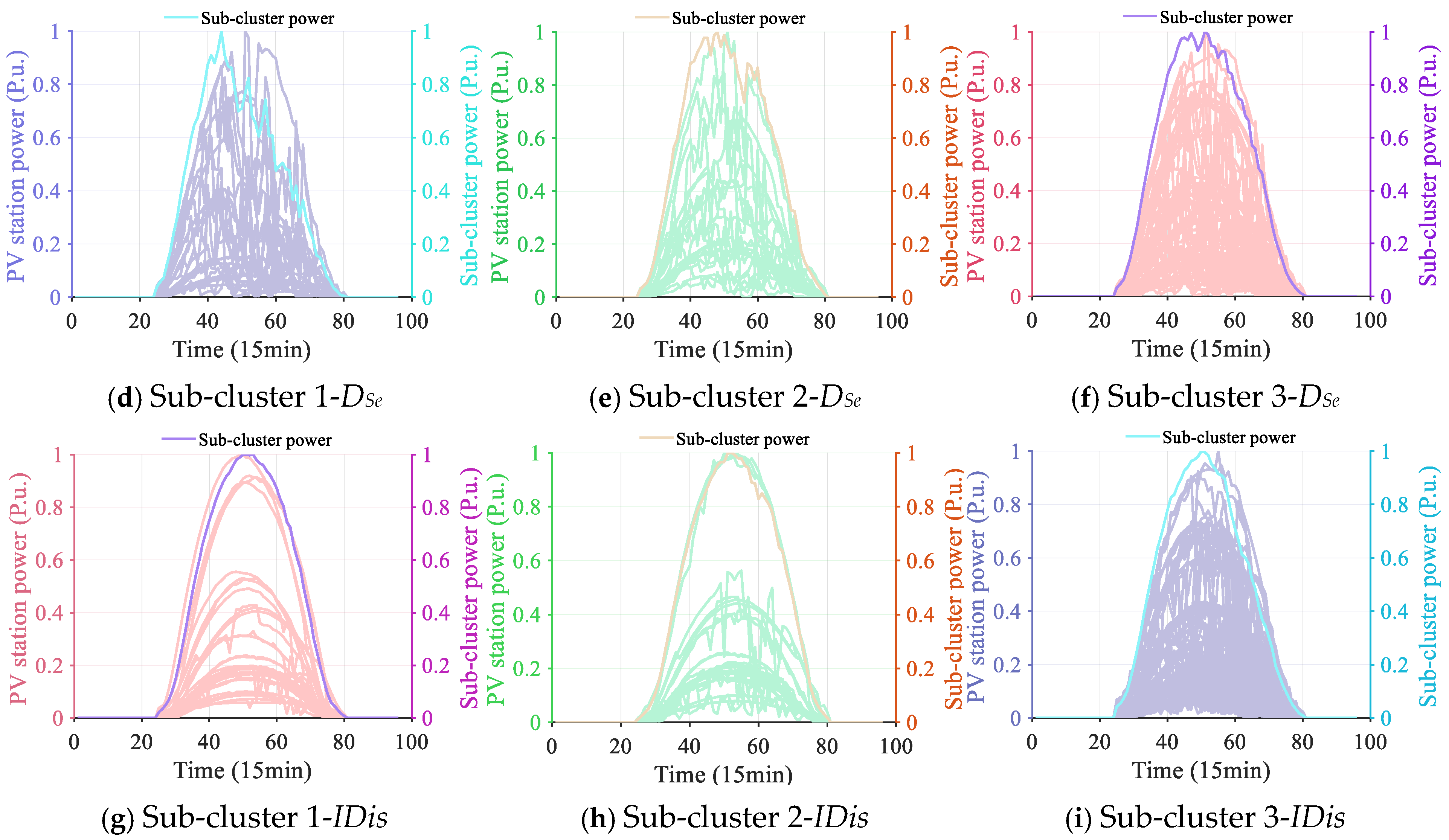
Figure 6a–c present the sub-clusters obtained with the correlation-coefficient criterion; each panel corresponds to one of three sub-clusters exhibiting distinct correlation signatures. In each sub-figure, the dense PV curves of the same color represent the individual PV power curves of the same sub-cluster after dynamic division of the PV cluster, corresponding to individual PV power stations. The thicker curves in another color represent the sum of the power of these PV power stations—the total power of the sub-cluster. Figure 6d–f illustrate the three sub-clusters derived from sample entropy similarity. Here, each group collects plants whose volatility magnitudes are comparable. Figure 6g–i display the three sub-clusters generated by the proposed volatility-smoothing mechanism. All three approaches successfully extract sub-clusters aligned with their respective criteria, yet the resulting volatility levels differ markedly. Sub-clusters based on correlation or sample entropy retain pronounced fluctuations. For example, sub-cluster 2 in the correlation-based division and sub-clusters 1 and 2 in the entropy-based division yield only marginal smoothing when their members are combined. By contrast, the divisions produced by the proposed volatility-smoothing criterion substantially attenuate intra-cluster volatility. After appropriate aggregation, the three sub-clusters deliver the smoothest possible composite signal—an outcome that is pivotal for enhancing PV cluster predictability.
In response to this, this section further compares the fluctuation levels of sub-clusters within the three clusters obtained after clustering under three clustering distance conditions using deep attention embedding graph clustering (DAEGC), spectral clustering models, and the k-means model used in this paper. This section primarily employs permutation entropy (Pe) as an indicator to describe the fluctuation levels of sub-cluster power. As shown in Table 3, DAEGC can only achieve clustering of similar samples based on Kullback–Leibler divergence, resulting in each clustering cluster containing only samples with similar fluctuations or similar fluctuation amplitudes at the PV station level. This leads to extreme situations in the corresponding three sub-clusters: some sub-clusters have extremely low Pe values with minimal complexity, primarily consisting of clear-sky weather samples, while others exhibit extremely high fluctuations for power, primarily comprising high-variability samples. When using sample entropy and correlation coefficients as clustering distances, the results are similar because the clustering model tends to cluster samples with similar volatility and similar trends into the same cluster. As a result, some sub-clusters may exhibit abnormally high fluctuations for power, while others may exhibit abnormally low power fluctuations. The improved clustering distance proposed in this paper clusters sub-clusters with volatility-smoothing characteristics into the same cluster, ensuring that each PV sample within a sub-cluster exhibits a significant increase in smoothness after superposition. For example, the complexity (Pe) of the sub-clusters obtained after applying the spectral clustering model based on improved clustering distance and the k-means model averaged only 0.3829 and 0.3819, respectively. However, other clustering distances exhibited varying performance across different models, with the clustering method based on DAEGC achieving the highest average complexity—an average Pe of 0.6788. The clustering method based on the improved clustering distance resulted in an average Pe for each sub-cluster that was 0.2831 lower than that of the other clustering methods. Therefore, the clustering methods and models proposed in this paper can be used to obtain sub-clusters with the lowest volatility in real time, thereby enhancing the predictability of PV cluster power.
Table 4 reports the error metrics for all models under the three dynamic division scenarios. Relative to static cluster division, any form of dynamic clustering improves predictive accuracy: real-time re-clustering continuously corrects system-level deviations caused by local volatility or time-varying effects, ensuring that the sub-clusters remain congruent with their instantaneous evolution characteristics. Consequently, all three dynamic schemes enhance PV cluster forecasting skill, yet they differ in the magnitude and mechanism of improvement. Divisions based on correlation or sample entropy similarity group stations with comparable evolution trends or volatility magnitudes. Within such sub-clusters, however, the stations merely replicate a common pattern and provide little additional information for boosting accuracy; the resulting gains are therefore limited. By contrast, the division based on aggregation smoothing explicitly exploits power-smoothing synergies: the strategic superposition of appropriately selected plants yields markedly smoother sub-cluster signals, directly enhancing predictability. Relative to the static division, the proposed smoothing-aware scheme reduces PV clusters NRMSE and NMAE by 1.29% and 0.68% on average, while raising R2 by 8.20%. Compared with the correlation and entropy-based dynamic division, the reductions in NRMSE and NMAE reach 2.12% and 0.51%, respectively, and R2 rises by 7.15%. Thus, the aggregation-smoothing function delivers a substantial accuracy gain. Regardless of the division paradigm, BITCN and Transformer consistently outperform traditional baselines, with BITCN achieving the lowest errors. Deep-learning architectures readily capture fine-grained power and meteorological fluctuations. BITCN, by virtue of its bidirectional temporal modeling, is particularly adept at learning ultra-short-term evolution patterns, yielding the most accurate forecasts.

3.4. Performance Comparison of the STHDGCN-BITCN Combined Model Across Different Clustering Methods

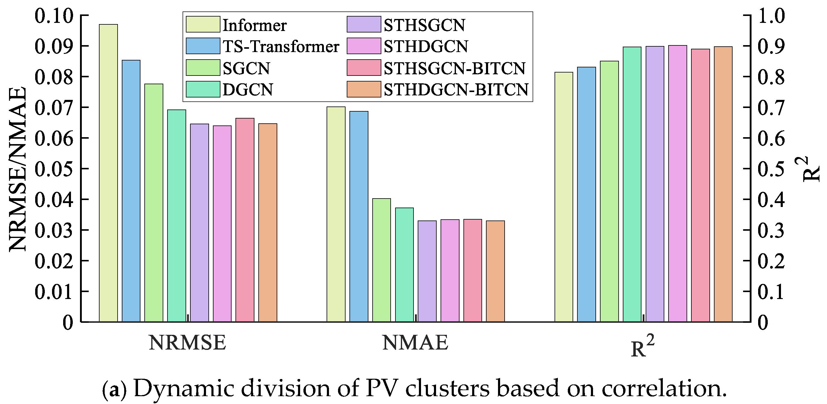
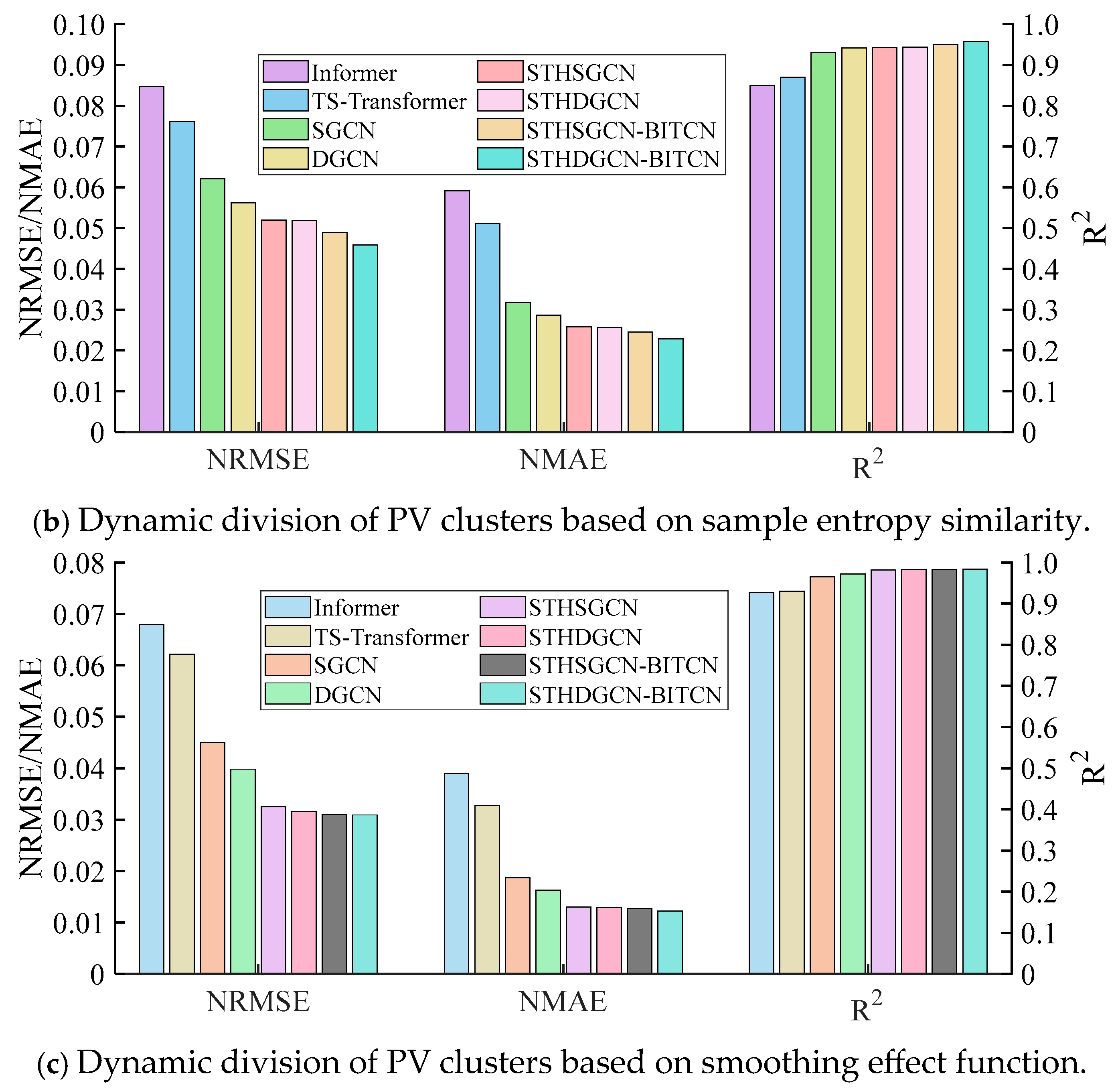
Ablation experiment (3) systematically contrasts the forecasting performance of static and dynamic graph convolution networks, static and dynamic spatiotemporal heterogeneous graph convolution networks, and their BITCN-augmented counterparts under each of the three dynamic division mechanisms. Figure 7 shows the error metrics for every model based on graphs across the three clustering schemes. Irrespective of the division strategy, graph neural network models consistently outperform conventional baselines. Across all three dynamic-clustering scenarios, the NRMSE and NMAE of every graph network are on average 3.83% and 1.88% lower, respectively, than those of the best traditional model under the same division, while R2 improves by 13.45%. Relative to the full set of classical cluster modeling paradigms (holistic approach, cumulative method, statistical upscaling, and static cluster division), the graph-based models reduce NRMSE and NMAE by 4.81% and 2.84% on average, and R2 rises by 29.75%. When the proposed aggregation-smoothing-based dynamic clustering is combined with a graph network, the gains widen further: compared with the best traditional model under the same clustering, NRMSE and NMAE fall by 5.51% and 2.98%, and R2 climbs by 17.53%. Relative to the classical cluster modeling paradigms, the reductions reach 6.49% and 3.94%, and R2 increases by 33.84%. In short, graph neural network modeling markedly improves accuracy regardless of whether the benchmark is classical cluster modeling or any static/dynamic division scheme.
Among the three dynamic cluster divisions, the proposed aggregation-smoothing function delivers the largest error reductions. Graph networks rely on an adjacency matrix to encode spatiotemporal fusion; when edges are defined by correlation coefficients, the representation suffers from a critical drawback. Correlation captures state similarity, so highly correlated nodes already carry redundant information, and graph-convolutional aggregation yields limited additional signals. The observed accuracy gain therefore originates almost entirely from the dynamic clustering itself, not from richer feature fusion. Sample-entropy similarity, by contrast, links nodes with comparable fluctuation magnitudes. Although this improves performance over conventional baselines, the benefit stems primarily from training on more homogeneous samples rather than from true information expansion. Based on this, this paper uses BITCN combined with spatiotemporal heterogeneous dynamic graph convolutional networks for cluster prediction. To compare the advantages of this combined model, this section introduces models such as SGCN, DGCN, STHSGCN, STHDGCN, STHSGCN-BITCN, STHDGCN-BITCN, Informer [78], and spatiotemporal Transformer (ST-Transformer) [79] for comparative analysis.
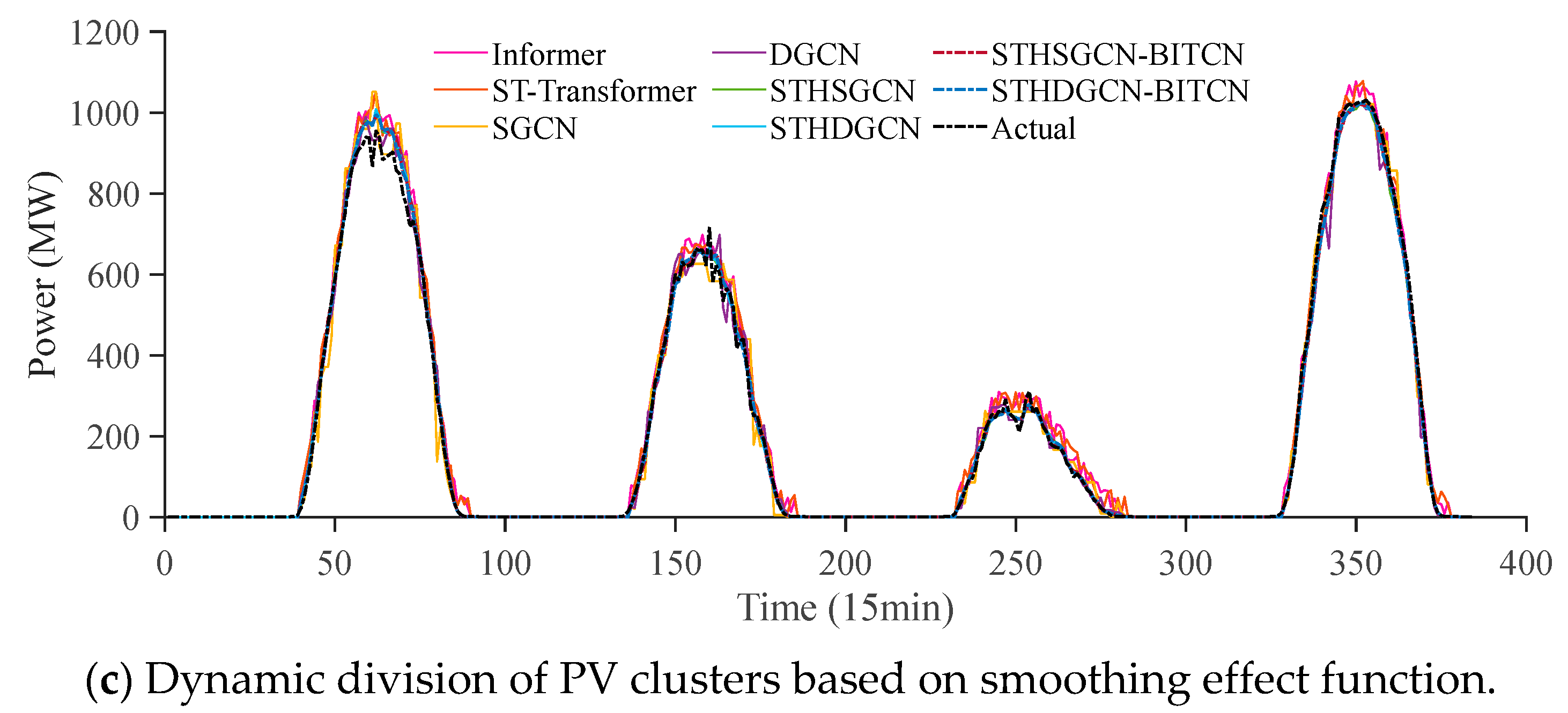
As shown in Figure 7, the aggregation-smoothing clusters exhibit pronounced volatility suppression: strategic superposition of plant-level power markedly flattens sub-cluster signals. Consequently, smoother sequences enter the graph network, furnishing inherently more predictable node features. Relative to correlation-based clustering, the proposed method lowers the NRMSE and NMAE of every graph-based model by 3.26% and 2.07% on average, while R2 rises by 8.89%. Compared with sample-entropy-based clustering, the reductions are 1.77% and 1.22%, and R2 improves by 3.36%. It is worth noting that, although Informer and ST-Transformer exhibit strong temporal prediction performance, their modeling accuracy is significantly lower than that of graph modeling methods based on STHSGCN and STHDGCN, as these models do not account for the multi-level heterogeneous relationships within PV clusters. Considering spatiotemporal modeling performance, ST-Transformer achieves higher prediction accuracy than Informer. Among the three cluster division methods, the average prediction NRMSE of ST-Transformer is 2.06%, 3.12%, and 3.02% higher than the proposed method, respectively, while the average NMAE is 3.56%, 2.84%, and 2.06% higher than the proposed method, respectively. Meanwhile, the average R2 is 6.67%, 8.73%, and 5.33% lower than the proposed method, respectively.
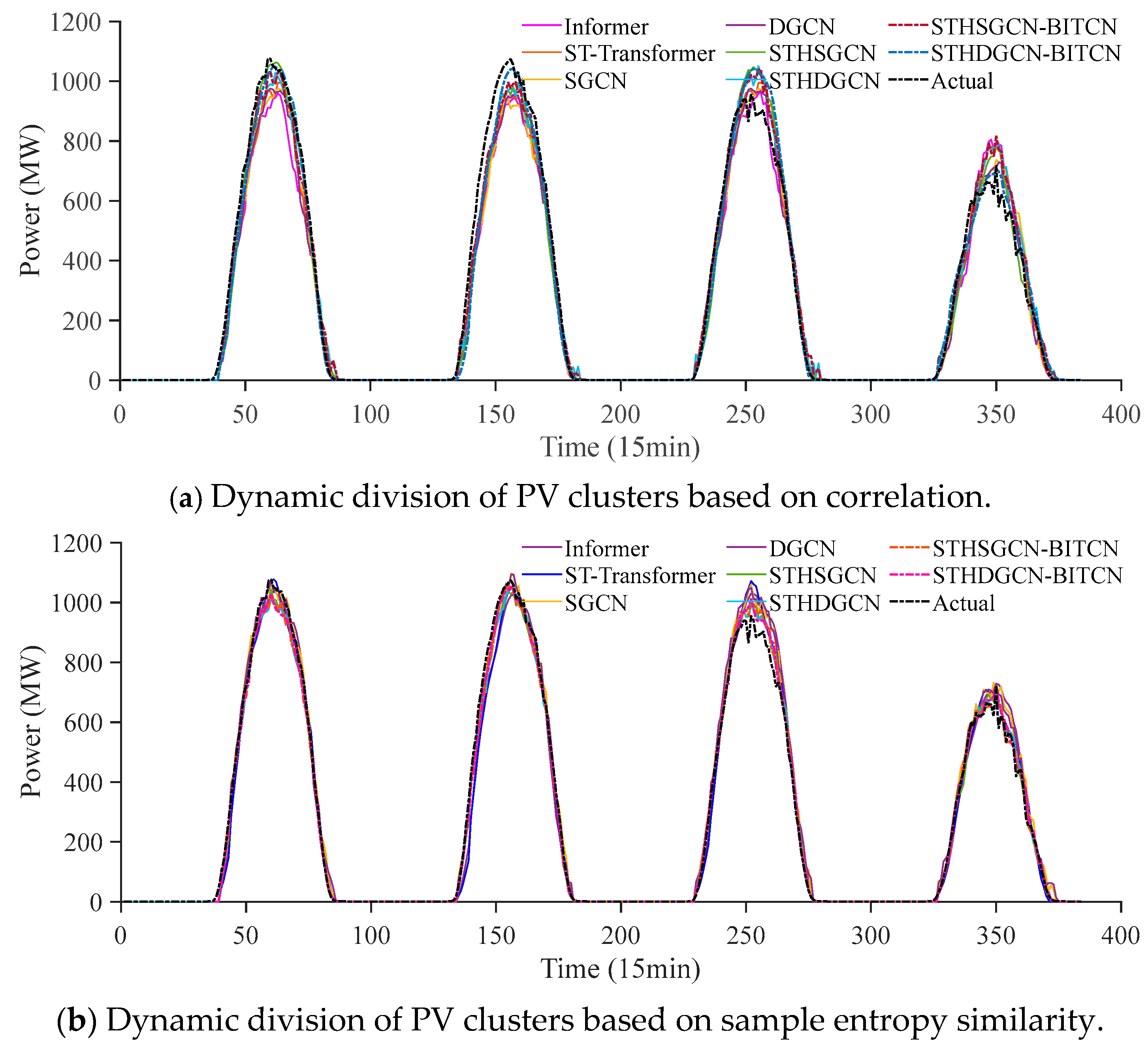
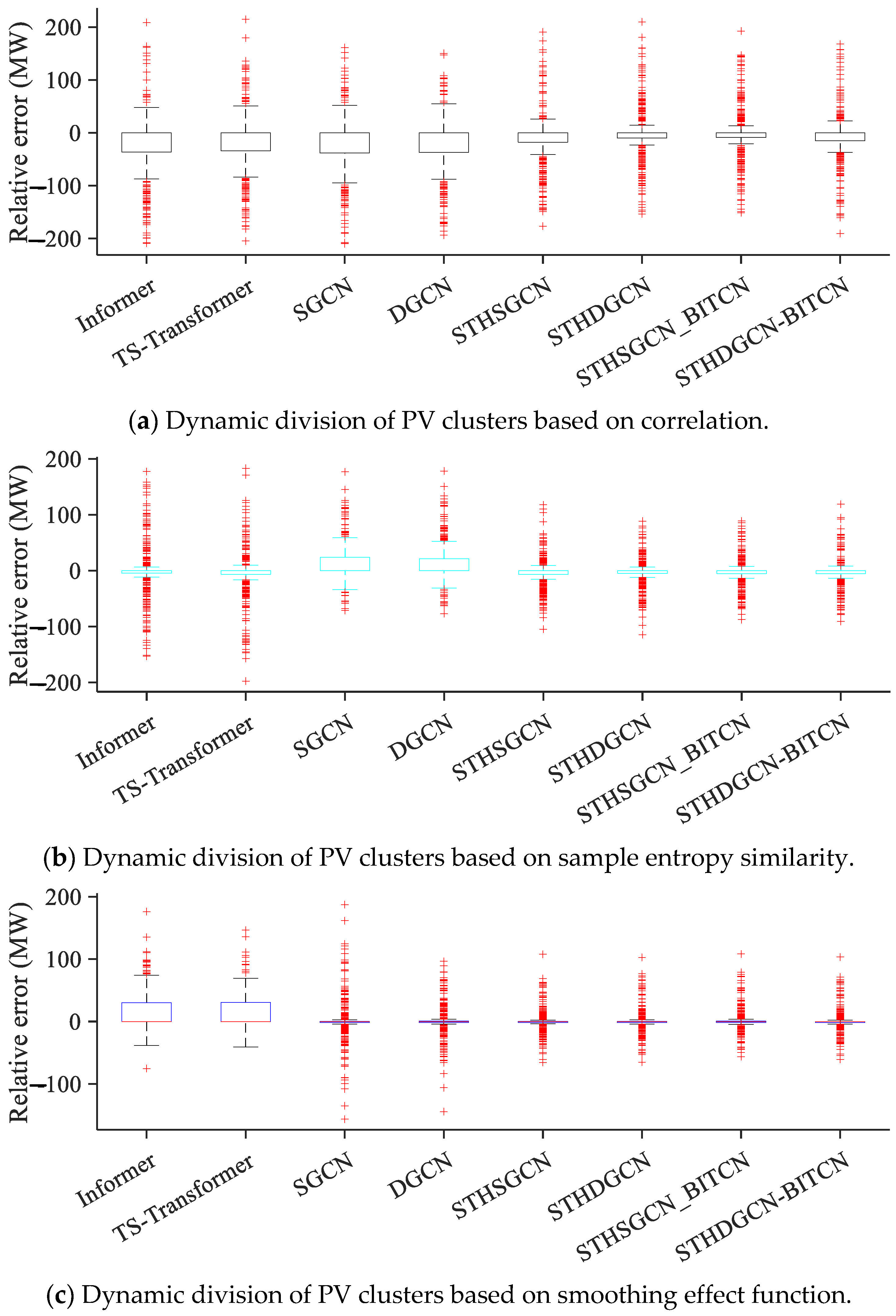
Across graph architectures, modeling accuracy diverges significantly. Conventional GCNs rely on a single-graph topology, which may inadequately represent the multiplicity of node–node relationships. Heterogeneous GCNs remedy this limitation by exploiting multiple distinct edge types, thereby flexibly capturing diverse spatiotemporal dependencies. The present study employs three heterogeneous graphs—trend correlation, amplitude similarity, and volatility similarity—that jointly encode the full spectrum of fluctuation relationships. Across all three clustering schemes, heterogeneous architectures yield the lowest errors: relative to conventional GCN, NRMSE and NMAE fall by 0.96% and 0.53%, and R2 rises by 1.63%. Dynamic graphs consistently outperform their static counterparts because they adapt to the cluster’s evolving state. Relative to static graphs, dynamic topologies reduce NRMSE and NMAE by 0.29% and 0.12%, and increase R2 by 0.91%. Augmenting the STHDGCN with a BITCN further sharpens temporal pattern extraction: compared with all other graph-based variants, NRMSE and NMAE drop by 0.59% and 0.32%, and R2 improves by 0.94%. In aggregate, the proposed combination of aggregation-smoothing dynamic clustering with a STHDGCN yields the largest error reductions. Relative to every competing model–division combination, NRMSE and NMAE are on average 3.12% and 1.97% lower, and R2 is 7.00% higher. Compared with the cluster modeling paradigms, the reductions reach 6.90% and 4.15%, and R2 increases by 34.36%. Relative to traditional models under the alternative dynamic partitions, the decreases are 6.63% and 3.36%, and R2 rises by 20.44%. Figure 8 superimposes the forecast traces of representative days for each clustering strategy and model. Regardless of the division scheme, every graph-based model tracks the true curve far more closely than any traditional baseline under the classical cluster modeling paradigms. Figure 5 and Figure 8 jointly demonstrate that the proposed aggregation-smoothing clustering methods, coupled with the STHDGCN, leverage multiple heterogeneous fluctuation graphs and bidirectional temporal modeling to deliver a substantial and consistent improvement in PV cluster power forecasting. Figure 9 further shows the distribution of prediction errors corresponding to different prediction models and cluster division methods. It is clear that the modeling method proposed in this paper, based on spatiotemporal heterogeneous graphs combined with BITCN, can significantly improve prediction errors and achieve high prediction accuracy.

4. Discussion and Analysis

This paper proposes a volatility-smoothing convergence-based dynamic clustering strategy for PV clusters and couples it with a STHDGCN integrated with BITCN to mine the spatiotemporal evolution of PV cluster power. The following subsections contrast the proposed pipeline with conventional modeling approaches in terms of computational overhead, engineering feasibility, and robustness under extreme scenarios.

4.1. Modeling Cost Analysis

The proposed workflow involves two main stages: (1) dynamic clustering based on a volatility-smoothing metric and (2) joint forecasting via STHDGCN-BITCN. To evaluate computational efficiency, Table 5 compares its time consumption against traditional clustering paradigms: the holistic approach, cumulative method, statistical upscaling, and static cluster division. The cumulative method builds a prediction model per PV station and aggregates their outputs, with training time equal to the sum of individual model trainings. The holistic method treats the PV cluster as a single entity, requiring only one model, with modeling cost similar to that of one station under the cumulative approach. Statistical upscaling identifies a representative plant within the PV cluster, models its power, and scales it to the PV cluster level, incurring a modeling cost comparable to one plant in the cumulative method. Static cluster division identifies sub-clusters using similarity measures (e.g., Pearson correlation), models each separately, and aggregates their predictions—modeling cost depends on the number of sub-clusters, though division itself is not time-consuming. The proposed method uses dynamic clustering, constructs spatiotemporal heterogeneous graphs, and employs graph attention networks to process all nodes simultaneously, enabling single-step prediction of all sub-clusters and significantly reducing training time. Since training occurs offline and prediction online, the online prediction time remains low across methods.
The cumulative method necessitates individual models per PV station, resulting in linearly increasing costs with cluster size and the highest expense. The holistic approach treats the entire PV cluster as a single entity, requiring only one model and thus being the cheapest. Statistical upscaling uses representative plants and also trains one model, maintaining low overhead. Static cluster division classifies plants with negligible time but trains a separate model per sub-cluster, so cost increases with cluster count, though remaining slightly below full summation. The proposed method spends more time on dynamic clustering, yet employs a single STHDGCN-BITCN model for joint prediction of all nodes, so training and inference times are independent of cluster count. Overall, its offline cost exceeds the holistic and statistical upscaling methods by 465.2 s on average, but remains significantly below cumulative summation and is comparable to static clustering. During online operation, pre-trained models impose negligible latency. Thus, despite a marginally higher upfront cost than two benchmarks, it achieves substantial accuracy gains, offering a favorable trade-off between computational cost and predictive performance, demonstrating strong engineering viability and practical advantage.

4.2. Error Behavior Under Extreme Conditions

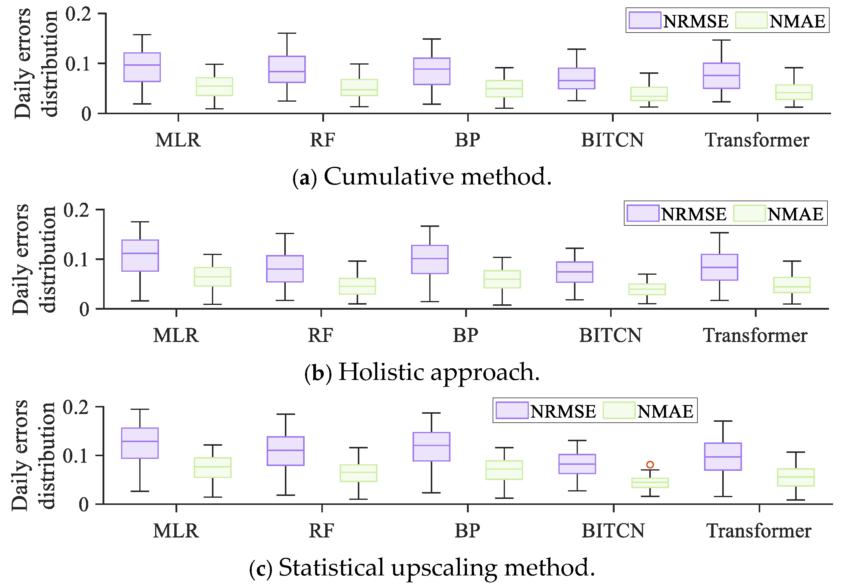
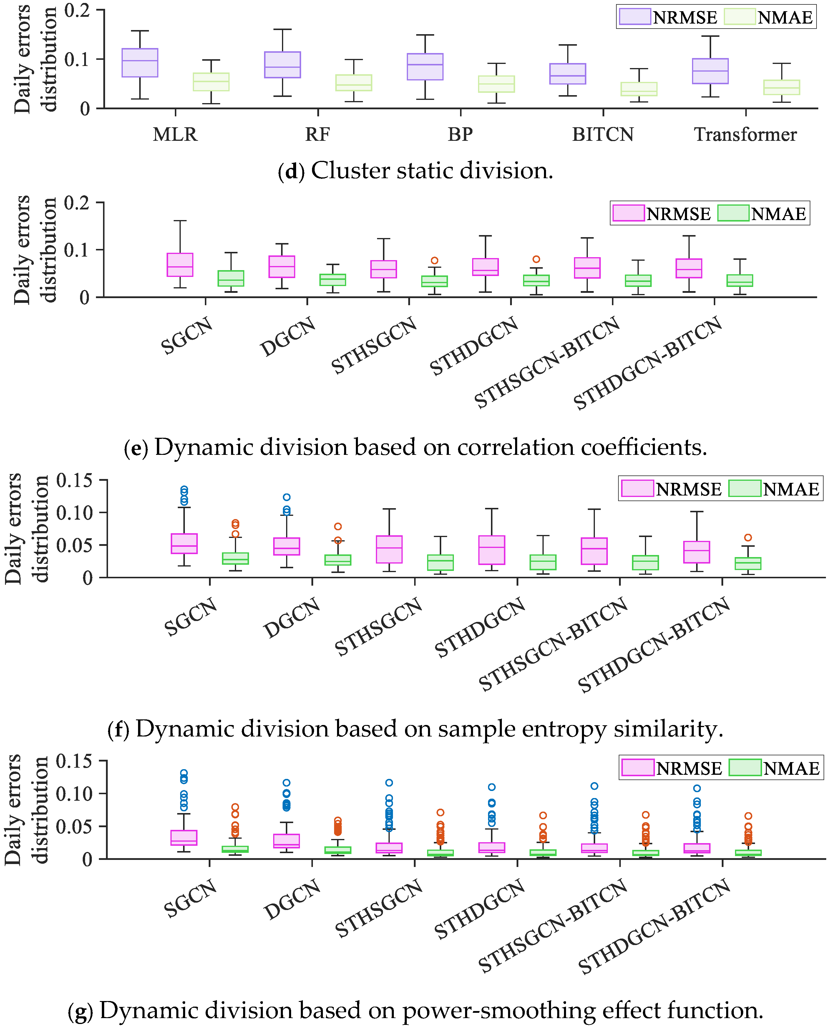
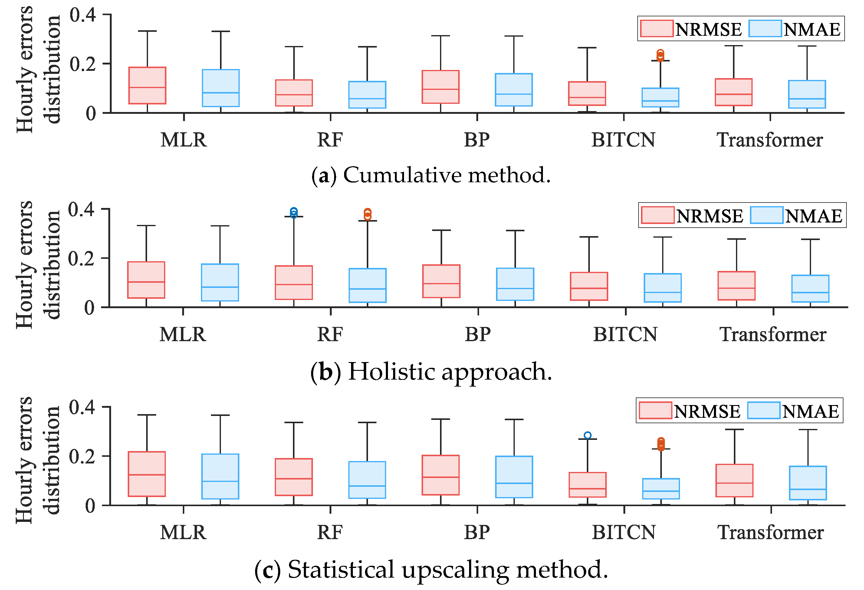
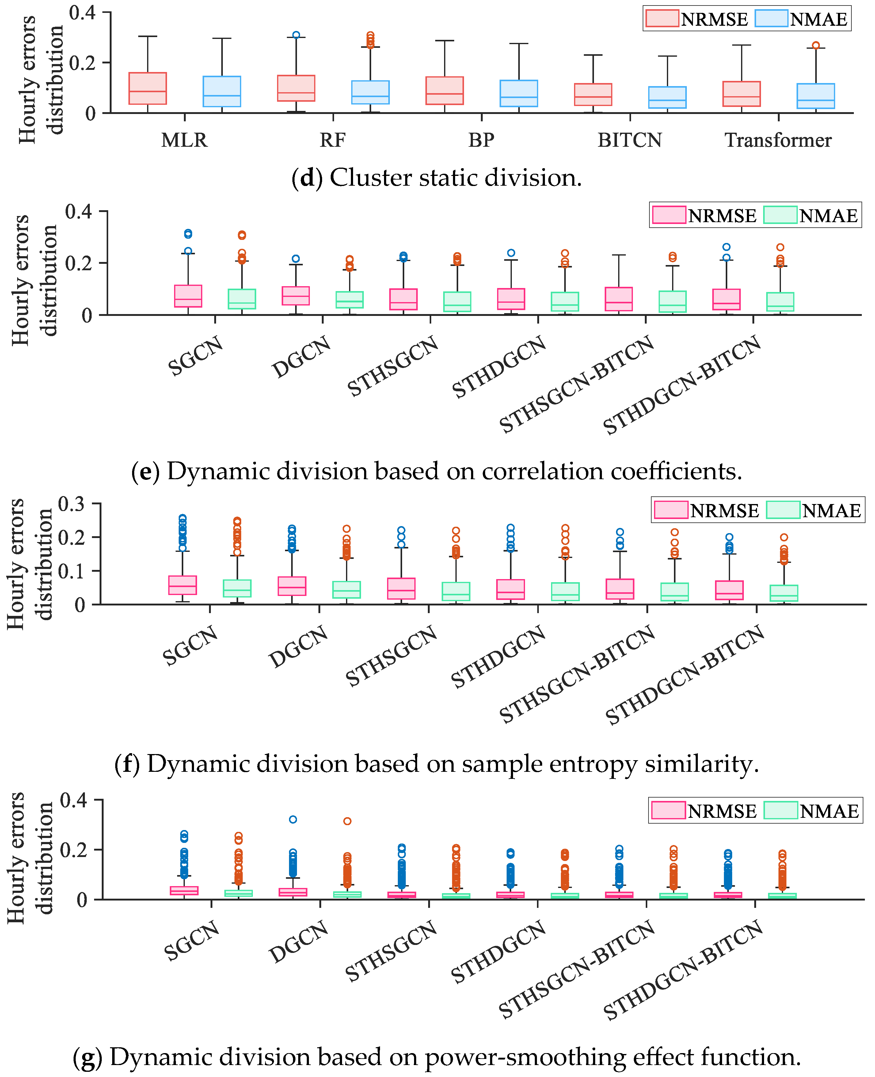
Although the proposed method achieves a substantial overall accuracy gain—reducing fleet-level NRMSE and NMAE by 6.90% and 4.15%, respectively, and raising R2 by 34.36% relative to traditional paradigms—local errors during extreme episodes remain a critical evaluation criterion. This subsection therefore compares the daily and hourly error distributions of conventional prediction models and the proposed model across all clustering strategies. Figure 10 presents the daily error distributions. Traditional single-node models applied to classical schemes (holistic approach, cumulative method, statistical upscaling, and static cluster division; Figure 10a–d) exhibit pronounced error tails. NRMSE is typically concentrated between 9% and 11%, with extreme values reaching 18%; NMAE clusters around 5–8%, with spikes up to 12%. Dynamic clustering markedly tightens these distributions (Figure 10e,f): under both alternative and proposed division mechanisms, NRMSE now centers on 5–6%, with extremes at 16%, while NMAE centers on 3–4%, with extremes at 10%.
Figure 11 displays the corresponding hourly error distributions (night-time excluded). Within classical paradigms (Figure 11a–d), individual models exhibit pronounced extremes: NRMSE averages 8–10%, but tail events exceed 30%, and minima can fall to 0; NMAE averages 5–8%, with similar tails. Under the proposed model combined with alternative dynamic division, hourly NRMSE still averages 8–10%, with 30% extremes, and NMAE averages 4–7%. Yet the proposed aggregation-smoothing dynamic clustering shifts the bulk of the distribution significantly downward: hourly NRMSE centers near 3% and NMAE near 2%. Both daily and hourly errors are confined to the narrowest ranges observed, clearly outperforming traditional paradigms and all alternative dynamic divisions. Thus, even under extreme conditions, the proposed method retains marked robustness and practical feasibility.

5. Conclusions

This paper proposes a dynamic PV cluster division method based on a volatility–convergence-smoothing mechanism. It constructs a hybrid forecasting framework integrating a spatiotemporal dynamic graph convolutional network with multi-relationships and a bidirectional temporal convolutional neural network, thereby enabling the capture of dynamic evolutionary patterns within individual sub-cluster nodes. We design three novel fluctuation-aware heterogeneous graphs to represent the evolving trends within PV sub-clusters, which establish multiple inter-cluster connections and significantly improve the accuracy of PV cluster power prediction. The integrated aggregation-smoothing dynamic clustering with STHDGCN achieves the highest predictive performance, significantly outperforming all conventional and alternative methods with the greatest improvements in NRMSE, NMAE, and R2 across all comparisons—notably reducing NRMSE and NMAE by 6.90% and 4.15% and increasing R2 by 34.36% compared to traditional cluster prediction paradigms.
Although the proposed framework markedly improves PV cluster prediction accuracy while balancing computational cost, its reliance on volatility–convergence characteristics may limit its effectiveness in small-scale PV clusters where smoothing opportunities are sparse. Future work will therefore investigate how to leverage convergence effects in such scenarios to further enhance forecasting performance.

Author Contributions

Y.L.: methodology, software, data curation, and writing—review and editing. M.Y.: methodology. Conceptualization, Y.L.; methodology, Y.L.; software, Y.L.; validation, Y.L. and M.Y.; formal analysis, Y.L.; investigation, Y.L.; resources, M.Y.; data curation, Y.L.; writing—original draft preparation, M.Y.; writing—review and editing, Y.L.; visualization, Y.L.; supervision, M.Y.; project administration, M.Y.; funding acquisition, Y.L. All authors have read and agreed to the published version of the manuscript.

Funding

This research is funded by Analysis and application of spatiotemporal evolution law of long-period process of extreme weather and its influence on new energy operation (4000-202455070A-1-1-ZN).

Data Availability Statement

Data are unavailable due to privacy or ethical restrictions.

Conflicts of Interest

The authors declare that the research was conducted in the absence of any commercial or financial relationships that could be construed as potential conflicts of interest.

Abbreviations

The following abbreviations are used in this manuscript:
PVPhotovoltaic
PCPPPhotovoltaic cluster power prediction
NWPNumerical Weather Prediction
PePermutation entropy
R2Coefficient of determination
NRMSENormalized root mean square error
NMAENormalized mean absolute error
k-meansk-mean clustering
BPBack propagation neural network
RFRandom forests
MLRMultiple linear regression
TCNTemporal convolutional neural network
GRUGate recurrent unit neural network
BITCNBidirectional temporal convolutional neural network
GNNGraph neural network
SGCNStatic graph convolutional network
DGCNDynamic graph convolutional network
STHSGCNSpatiotemporal heterogeneous static graph convolutional network
STHDGCNSpatiotemporal heterogeneous dynamic graph convolutional neural network
TransformerTransformer neural network
InformerInformer neural network
ST-TransformerSpatiotemporal Transformer neural network
STHSGCN-BITCNSTHSGCN combined with BITCN
STHDGCN-BITCNSTHDGCN combined with BITCN

References

  1. Dong, Y.; Li, W.; Zhang, J.; Luo, W.; Fu, H.; Xin, X.; Hu, P.; Dong, Y.; Tan, J. High-speed PGC demodulation model and method with subnanometer displacement resolution in a fiber-optic micro-probe laser interferometer. Photonics Res. 2024, 12, 921–931. [Google Scholar] [CrossRef]
  2. Zhang, C.; Dong, Y.; Hu, P.; Fu, H.; Yang, H.; Yang, R.; Dong, Y.; Zou, L.; Tan, J. Large-range displacement measurement in narrow space scenarios: Fiber microprobe sensor with subnanometer accuracy. Photonics Res. 2024, 12, 1877–1889. [Google Scholar] [CrossRef]
  3. Zhang, N.; Yan, J.; Hu, C.; Sun, Q.; Yang, L.; Gao, D. Price-matching-based regional energy market with hierarchical reinforcement learning algorithm. IEEE Trans. Ind. Inform. 2024, 20, 11103–11114. [Google Scholar] [CrossRef]
  4. Soares, A.; Gomes, Á.; Antunes, C.H.; Oliveira, C. A customized evolutionary algorithm for multiobjective management of residential energy resources. IEEE Trans. Ind. Inform. 2016, 13, 492–501. [Google Scholar] [CrossRef]
  5. Zhang, B.; Talihati, B.; Fan, H.; Sun, Y.; Wang, Y. A dynamic carbon flow traceability framework for integrated energy systems. J. Clean. Prod. 2025, 518, 145878. [Google Scholar] [CrossRef]
  6. Meng, Q.; He, Y.; Li, S.; Hussain, S.; Lu, J.; You, G.; Guerrero, J. Adaptive two-step power prediction and improved perturbation method for accelerated MPPT with reduced oscillations in photovoltaic systems. Energy Rep. 2025, 13, 5328–5338. [Google Scholar] [CrossRef]
  7. Gao, J.; Tian, S.; Yuan, C.; Ma, Z.; Gao, C.; Yan, G. Design and optimization of a novel double-layer Helmholtz coil for wirelessly powering a capsule robot. IEEE Trans. Power Electron. 2023, 39, 1826–1839. [Google Scholar] [CrossRef]
  8. Wang, Z.; Zhang, C.; Chen, Z.; Hu, W.; Lu, K.; Ge, L. ACR-Net: Learning high-accuracy optical flow via adaptive-aware correlation recurrent network. IEEE Trans. Circuits Syst. Video Technol. 2024, 34, 9064–9077. [Google Scholar] [CrossRef]
  9. Wang, Q.; Luo, R.; Wang, Y.; Fang, W.; Jiang, L.; Liu, Y.; Wang, R.; Dai, L.; Zhao, J.; Bai, J.; et al. Set/Reset bilaterally controllable resistance switching Ga-doped Ge2Sb2Te5 long-term electronic synapses for neuromorphic computing. Adv. Funct. Mater. 2023, 33, 2213296. [Google Scholar] [CrossRef]
  10. Yang, Z.; Huo, S.; Zhang, Z.; Meng, F.; Liu, B.; Wang, Y.; Ma, Y.; Wang, Z.; Xu, J.; Tian, Q.; et al. High—Precision Multibit Opto—Electronic Synapses Based on ReS2/h-BN/Graphene Heterostructure for Energy-Efficient and High-Accuracy Neuromorphic Computing. Adv. Funct. Mater. 2025, 2509119, Early View. [Google Scholar] [CrossRef]
  11. AlKandari, M.; Ahmad, I. Solar power generation forecasting using ensemble approach based on deep learning and statistical methods. Appl. Comput. Inform. 2024, 20, 231–250. [Google Scholar] [CrossRef]
  12. Zhang, Y.; Zhang, Y.; Zheng, B.; Cui, H.; Qi, H. Statistical analysis for estimating the optimized battery capacity for roof-top PV energy system. Renew. Energy 2025, 242, 122491. [Google Scholar] [CrossRef]
  13. Mayer, M.J.; Gróf, G. Extensive comparison of physical models for photovoltaic power forecasting. Appl. Energy 2021, 283, 116239. [Google Scholar] [CrossRef]
  14. Yang, M.; Jiang, Y.; Zhang, W.; Li, Y.; Su, X. Short-term Interval Prediction Strategy of Photovoltaic Power Based on Meteorological Reconstruction with Spatiotemporal Correlation and Multi-factor Interval Constraints. Renew. Energy 2024, 237, 121834. [Google Scholar] [CrossRef]
  15. Yang, M.; Jiang, Y.; Guo, Y.; Li, Y.; Huang, T. Ultra-short-term Prediction of Photovoltaic Cluster Power Based on Spatiotemporal Convergence Effect and Spatiotemporal Dynamic Graph Attention Network. Renew. Energy 2025, 255, 123843. [Google Scholar] [CrossRef]
  16. Yuqi, J.; An, A.; Lu, Z.; He, P.; Liu, X. Short-term load forecasting based on temporal importance analysis and feature extraction. Electr. Power Syst. Res. 2025, 244, 111551. [Google Scholar] [CrossRef]
  17. Yang, M.; Zhao, M.; Huang, D.; Su, X. A composite framework for photovoltaic day-ahead power prediction based on dual clustering of dynamic time warping distance and deep autoencoder. Renew. Energy 2022, 194, 659–673. [Google Scholar] [CrossRef]
  18. Yang, M.; Guo, Y.; Fan, F.; Huang, T. Two-stage correction prediction of wind power based on numerical weather prediction wind speed superposition correction and improved clustering. Energy 2024, 302, 131797. [Google Scholar] [CrossRef]
  19. Mayer, M.J.; Yang, D.; Markovics, D. The complexity and dimensionality of making deterministic photovoltaic power forecasts from ensemble numerical weather prediction. Energy Convers. Manag. 2025, 344, 120303. [Google Scholar] [CrossRef]
  20. Zjavka, L. Power Quality 24 h Verification in Smart Load Scheduling Based on Differentiate, Deep, and Assembly Statistics in NWP Processing. Int. Trans. Electr. Energy Syst. 2025, 2025, 8703225. [Google Scholar] [CrossRef]
  21. Yang, M.; Guo, Y.; Huang, T.; Fan, F.; Ma, C.; Fang, G. Wind farm cluster power prediction based on graph deviation attention network with learnable graph structure and dynamic error correction during load peak and valley periods. Energy 2024, 312, 133645. [Google Scholar] [CrossRef]
  22. Yang, M.; Guo, Y.; Wang, B.; Wang, Z.; Chai, R. A day-ahead wind speed correction method: Enhancing wind speed forecasting accuracy using a strategy combining dynamic feature weighting with multi-source information and dynamic matching with improved similarity function. Expert Syst. Appl. 2025, 263, 125724. [Google Scholar] [CrossRef]
  23. Yang, M.; Guo, Y.; Huang, T.; Zhang, W. Power prediction considering NWP wind speed error tolerability: A strategy to improve the accuracy of short-term wind power prediction under wind speed offset scenarios. Appl. Energy 2025, 377, 124720. [Google Scholar]
  24. Yang, M.; Guo, Y.; Huang, Y. Wind power ultra-short-term prediction method based on NWP wind speed correction and double clustering division of transitional weather process. Energy 2023, 282, 128947. [Google Scholar] [CrossRef]
  25. Jackson, N.D.; Gunda, T. Evaluation of extreme weather impacts on utility-scale photovoltaic plant performance in the United States. Appl. Energy 2021, 302, 117508. [Google Scholar] [CrossRef]
  26. Zhai, C.; He, X.; Cao, Z.; Tankari, M.; Wang, Y.; Zhang, M. Photovoltaic power forecasting based on VMD-SSA-Transformer: Multidimensional analysis of dataset length, weather mutation and forecast accuracy. Energy 2025, 324, 135971. [Google Scholar] [CrossRef]
  27. Sánchez-Pozo, N.N.; Vanem, E.; Bloomfield, H.; Aizpurua, J. A probabilistic risk assessment framework for the impact assessment of extreme events on renewable power plant components. Renew. Energy 2025, 240, 122168. [Google Scholar] [CrossRef]
  28. Markovics, D.; Mayer, M.J. Comparison of machine learning methods for photovoltaic power forecasting based on numerical weather prediction. Renew. Sustain. Energy Rev. 2022, 161, 112364. [Google Scholar] [CrossRef]
  29. Yang, M.; Zhao, M.; Liu, D.; Ma, M.; Su, X. Improved Random Forest Method for Ultra-short-term Prediction of the Output Power of a Photovoltaic Cluster. Front. Energy Res. 2021, 9, 749367. [Google Scholar] [CrossRef]
  30. Pulipaka, S.; Kumar, R. Power prediction of soiled PV module with neural networks using hybrid data clustering and division techniques. Sol. Energy 2016, 133, 485–500. [Google Scholar] [CrossRef]
  31. Pang, S.; Zheng, Z.; Luo, F.; Xaio, X.; Xu, L. Hybrid forecasting methodology for wind power-photovoltaic-concentrating solar power generation clustered renewable energy systems. Sustainability 2021, 13, 6681. [Google Scholar] [CrossRef]
  32. Jin, J.; Ye, L.; Li, J.; Zhao, Y.; Lu, P.; Wang, W. Wind and photovoltaic power time series data aggregation method based on an ensemble clustering and Markov chain. CSEE J. Power Energy Syst. 2021, 8, 757–768. [Google Scholar] [CrossRef]
  33. Pierro, M.; De Felice, M.; Maggioni, E.; Moser, D.; Perotto, A.; Spada, F.; Cornaro, C. Data-driven upscaling methods for regional photovoltaic power estimation and forecast using satellite and numerical weather prediction data. Sol. Energy 2017, 158, 1026–1038. [Google Scholar] [CrossRef]
  34. Qiu, L.; Ma, W.; Feng, X.; Dai, J.; Dong, Y.; Duan, J.; Chen, B. A hybrid PV cluster power prediction model using BLS with GMCC and error correction via RVM considering an improved statistical upscaling technique. Appl. Energy 2024, 359, 122719. [Google Scholar] [CrossRef]
  35. Saint-Drenan, Y.M.; Good, G.H.; Braun, M.; Freisinger, T. Analysis of the uncertainty in the estimates of regional PV power generation evaluated with the upscaling method. Sol. Energy 2016, 135, 536–550. [Google Scholar] [CrossRef]
  36. Lai, W.; Zhen, Z.; Wang, F.; Fu, W.; Wang, J.; Zhang, X.; Ren, H. Sub-region division based short-term regional distributed PV power forecasting method considering spatio-temporal correlations. Energy 2024, 288, 129716. [Google Scholar] [CrossRef]
  37. Zhang, Z.; Lv, Q.; Zhang, J. Research on the combined power forecasting of regional wind and photovoltaic power based on statistical upscaling. In Proceedings of the 2nd International Conference on Mechanical, Electronics, and Electrical and Automation Control (METMS 2022), Guilin, China, 7–9 January 2022; SPIE: Bellingham, WA, USA; Volume 12244, pp. 1141–1147. [Google Scholar]
  38. Fu, L.; Yang, Y.; Yao, X.; Jiao, X.; Zhu, T. A regional photovoltaic output prediction method based on hierarchical clustering and the mRMR criterion. Energies 2019, 12, 3817. [Google Scholar] [CrossRef]
  39. Ziane, A.; Necaibia, A.; Sahouane, N.; Dabou, R.; Mostefaoui, M.; Bouraiou, A.; Khelifi, S.; Rouabhia, A.; Blal, M. Photovoltaic output power performance assessment and forecasting: Impact of meteorological variables. Sol. Energy 2021, 220, 745–757. [Google Scholar] [CrossRef]
  40. Meng, X.; Shi, X.; Wang, W.; Zhang, Y.; Gao, F. An upscaling minute-level regional photovoltaic power forecasting scheme. Int. J. Electr. Power Energy Syst. 2024, 155, 109609. [Google Scholar] [CrossRef]
  41. Wang, H.; Lu, Z.; Wojtasiak, A.; Owyong, S.; Sun, B.; Fang, Y.; Vassigh, S.; Lin, A. Biomimetic self-shading walls via 3D-printing for reduced heat gain: Multiscale learning using graph neural networks to predict solar radiation absorption. Build. Environ. 2025, 279, 113048. [Google Scholar] [CrossRef]
  42. Wang, S.; Xiang, X.; Zhang, J.; Liang, Z.; Li, S.; Zhong, P.; Zeng, J.; Wang, C. A multi-task spatiotemporal graph neural network for transient stability and state prediction in power systems. Energies 2025, 18, 1531. [Google Scholar] [CrossRef]
  43. Hassan, A.U.; Güleryüz, C.; El Azab, I.H.; Elnaggar, A.; Mahmoud, M. A graph neural network assisted reverse polymers engineering to design low bandgap benzothiophene polymers for light harvesting applications. Mater. Chem. Phys. 2025, 339, 130747. [Google Scholar] [CrossRef]
  44. Sun, D.; Cao, X.; Liang, Z.; Xia, J.; Wang, Y. Distributed Photovoltaic Power Prediction Technology Based on Spatio-Temporal Graph Neural Networks. Energy Eng. 2025, 122, 3329–3346. [Google Scholar] [CrossRef]
  45. Zhang, M.; Zhen, Z.; Liu, N.; Zhao, H.; Sun, Y.; Feng, C. Optimal graph structure based short-term solar PV power forecasting method considering surrounding spatio-temporal correlations. IEEE Trans. Ind. Appl. 2022, 59, 345–357. [Google Scholar] [CrossRef]
  46. Simeunović, J.; Schubnel, B.; Alet, P.; Carrillo, R.; Frossard, R. Interpretable temporal-spatial graph attention network for multi-site PV power forecasting. Appl. Energy 2022, 327, 120127. [Google Scholar] [CrossRef]
  47. Zhao, C.; Li, X.; Cai, Y. A power grid topology detection method based on edge graph attention neural network. Electr. Power Syst. Res. 2025, 239, 111219. [Google Scholar] [CrossRef]
  48. He, Y.; Ali, A.B.M.; Aminian, S.A.; Sharma, K.; Dixit, S.; Sobti, S.; Ali, R.; Ahemedei, M.; Rajab, H.; Mazinan, M. Enhancing Intelligent HVAC optimization with graph attention networks and stacking ensemble learning, a recommender system approach in Shenzhen Qianhai Smart Community. Sci. Rep. 2025, 15, 5119. [Google Scholar] [CrossRef]
  49. Abdelkader, D.; Fouzi, H.; Belkacem, K.; Ying, S. Graph neural networks-based spatiotemporal prediction of photovoltaic power: A comparative study. Neural Comput. Appl. 2025, 37, 4769–4795. [Google Scholar] [CrossRef]
  50. Simeunović, J.; Schubnel, B.; Alet, P.J.; Carrillo, R. Spatio-temporal graph neural networks for multi-site PV power forecasting. IEEE Trans. Sustain. Energy 2021, 13, 1210–1220. [Google Scholar] [CrossRef]
  51. Jiao, X.; Li, X.; Lin, D.; Xiao, W. A graph neural network based deep learning predictor for spatio-temporal group solar irradiance forecasting. IEEE Trans. Ind. Inform. 2021, 18, 6142–6149. [Google Scholar] [CrossRef]
  52. Yang, Y.; Liu, Y.; Zhang, Y.; Shu, S.; Zheng, J. DEST-GNN: A double-explored spatio-temporal graph neural network for multi-site intra-hour PV power forecasting. Appl. Energy 2025, 378, 124744. [Google Scholar] [CrossRef]
  53. Jing, S.; Xi, X.; Su, D.; Han, Z.; Wang, D. Spatio-Temporal Photovoltaic Power Prediction with Fourier Graph Neural Network. Electronics 2024, 13, 4988. [Google Scholar] [CrossRef]
  54. Zhang, X.; Gao, R.; Zhu, C.; Liu, C.; Mei, S. Ultra-short-term prediction of regional photovoltaic power based on dynamic graph convolutional neural network. Electr. Power Syst. Res. 2024, 226, 109965. [Google Scholar] [CrossRef]
  55. Li, Z.; Ye, L.; Song, X.; Luo, Y.; Pei, M.; Wang, K. Heterogeneous spatiotemporal graph convolution network for multi-modal wind-PV power collaborative prediction. IEEE Trans. Power Syst. 2023, 39, 5591–5608. [Google Scholar] [CrossRef]
  56. Hasnat, M.A.; Asadi, S.; Alemazkoor, N. A graph attention network framework for generalized-horizon multi-plant solar power generation forecasting using heterogeneous data. Renew. Energy 2025, 243, 122520. [Google Scholar] [CrossRef]
  57. Gao, Y.; Liang, L.; Su, T.; Pan, M. An embedded spatiotemporal hybrid model integrating multi-graphs and attention-driven fusion for single-and multi-site photovoltaic power forecasting. Energy Convers. Manag. 2025, 336, 119897. [Google Scholar] [CrossRef]
  58. Theiler, R.; Fink, O. Heterogeneous Graph Neural Networks for Short-term State Forecasting in Power Systems across Domains and Time Scales: A Hydroelectric Power Plant Case Study. arXiv 2025, arXiv:2507.06694. [Google Scholar] [CrossRef]
  59. Yang, K.; Cai, Y.; Cheng, J. A deep learning model based on multi-attention mechanism and gated recurrent unit network for photovoltaic power forecasting. Comput. Electr. Eng. 2025, 123, 110250. [Google Scholar] [CrossRef]
  60. Li, Z.; Ma, J.; Wang, Q.; Wang, M.; Jiang, F. Enhancing urban solar irradiation prediction with shadow-attention graph neural networks: Implications for net-zero energy buildings in New York City. Sustain. Cities Soc. 2025, 120, 106133. [Google Scholar] [CrossRef]
  61. Lin, H.; Gao, L.; Cui, M.; LIu, H.; Li, C.; Yu, M. Short-term distributed photovoltaic power prediction based on temporal self-attention mechanism and advanced signal decomposition techniques with feature fusion. Energy 2025, 315, 134395. [Google Scholar] [CrossRef]
  62. Zhang, C.; Song, D.; Huang, C.; Swami, A.; Chawla, N. Heterogeneous graph neural network. In Proceedings of the 25th ACM SIGKDD International Conference on Knowledge Discovery & Data Mining, Anchorage, AK, USA, 4–8 August 2019; pp. 793–803. [Google Scholar]
  63. Bing, R.; Yuan, G.; Zhu, M.; Meng, F.; Ma, H.; Qiao, S. Heterogeneous graph neural networks analysis: A survey of techniques, evaluations and applications. Artif. Intell. Rev. 2023, 56, 8003–8042. [Google Scholar] [CrossRef]
  64. Jing, Y.; Yang, Y.; Wang, X.; Song, M.; Tao, D. Amalgamating knowledge from heterogeneous graph neural networks. In Proceedings of the IEEE/CVF Conference on Computer Vision and Pattern Recognition, Nashville, TN, USA, 20–25 June 2021; pp. 15709–15718. [Google Scholar]
  65. Li, B.; Li, X.; Cai, Y.; Han, Q. A load forecasting method based on heterogeneous network for integrated electricity and heat systems. Electr. Power Syst. Res. 2025, 246, 111725. [Google Scholar] [CrossRef]
  66. Liu, Y.; Yang, M. Ultra-Short-Term Photovoltaic Power Prediction Based on Predictable Component Reconstruction and Spatiotemporal Heterogeneous Graph Neural Networks. Energies 2025, 18, 4192. [Google Scholar] [CrossRef]
  67. Xu, J.; Li, Y.; Lu, W.; Wu, S.; Li, Y. A heterogeneous traffic spatio-temporal graph convolution model for traffic prediction. Phys. A Stat. Mech. Its Appl. 2024, 641, 129746. [Google Scholar] [CrossRef]
  68. Liu, X.; Miao, C.; Fiumara, G.; Meo, P. Information propagation prediction based on spatial–temporal attention and heterogeneous graph convolutional networks. IEEE Trans. Comput. Soc. Syst. 2023, 11, 945–958. [Google Scholar] [CrossRef]
  69. Cai, S.; Zhao, Y.; Hu, Y.; Wu, J.; Wu, J.; Zhang, G.; Zhao, C.; Sosu, R. CD-BTMSE: A concept drift detection model based on bidirectional temporal convolutional network and multi-stacking ensemble learning. Knowl. Based Syst. 2024, 294, 111681. [Google Scholar] [CrossRef]
  70. Yang, M.; Ju, C.; Huang, Y.; Guo, Y.; Jia, M. Short-term power forecasting of wind farm cluster based on global information adaptive perceptual graph convolution network. IEEE Trans. Sustain. Energy 2024, 15, 2063–2076. [Google Scholar] [CrossRef]
  71. Gan, J.; Lin, X.; Chen, T.; Fan, C.; Wei, P.; Li, Z.; Huo, Y.; Zhang, F.; Liu, J.; He, T. Improving short-term photovoltaic power generation forecasting with a bidirectional temporal convolutional network enhanced by temporal bottlenecks and Attention Mechanisms. Electronics 2025, 14, 214. [Google Scholar] [CrossRef]
  72. Feng, Y.; Zhu, J.; Qiu, P.; Zhang, X.; Shuang, C. Short-term power load forecasting based on TCN-BiLSTM-attention and multi-feature fusion. Arab. J. Sci. Eng. 2025, 50, 5475–5486. [Google Scholar] [CrossRef]
  73. Zhu, H.; Wang, Y.; Wu, J.; Zhang, X. A regional distributed photovoltaic power generation forecasting method based on grid division and TCN-Bilstm. Renew. Energy 2026, 256, 123935. [Google Scholar] [CrossRef]
  74. Yang, M.; Guo, Y. Wind power cluster ultra-short-term prediction error correction method based on the load peak and valley characteristics. CSEE J. Power Energy Syst. 2023, 1–12. [Google Scholar] [CrossRef]
  75. Zhang, Z.; Liu, Z.; Ning, L.; Zhang, X. Belief-based fuzzy and imprecise clustering for arbitrary data distributions. IEEE Trans. Fuzzy Syst. 2025, 33, 2755–2767. [Google Scholar] [CrossRef]
  76. Zhang, Y.; Feng, S.; Wang, P.; Tan, Z.; Luo, X.; Ji, Y. Learning self-growth maps for fast and accurate imbalanced streaming data clustering. IEEE Trans. Neural Netw. Learn. Syst. 2025, 36, 16049–16061. [Google Scholar] [CrossRef] [PubMed]
  77. Zhou, C.; Zhang, F.; Gu, S.; Zhao, Z. A short-term power prediction method based on the transformation of multi-source spatiotemporal feature for photovoltaic cluster. Int. J. Green Energy 2025, 22, 2663–2679. [Google Scholar] [CrossRef]
  78. Yu, W.; Dai, Y.; Ren, T.; Leng, M. Short-time Photovoltaic Power Forecasting Based on Informer Model Integrating Attention Mechanism. Appl. Soft Comput. 2025, 178, 113345. [Google Scholar] [CrossRef]
  79. Tang, P.; Su, Y.; Zhao, W.; Wang, Q.; Zou, L.; Song, J. A Hybrid Framework for Photovoltaic Power Forecasting Using Shifted Windows Transformer-Based Spatiotemporal Feature Extraction. Energies 2025, 18, 3193. [Google Scholar] [CrossRef]
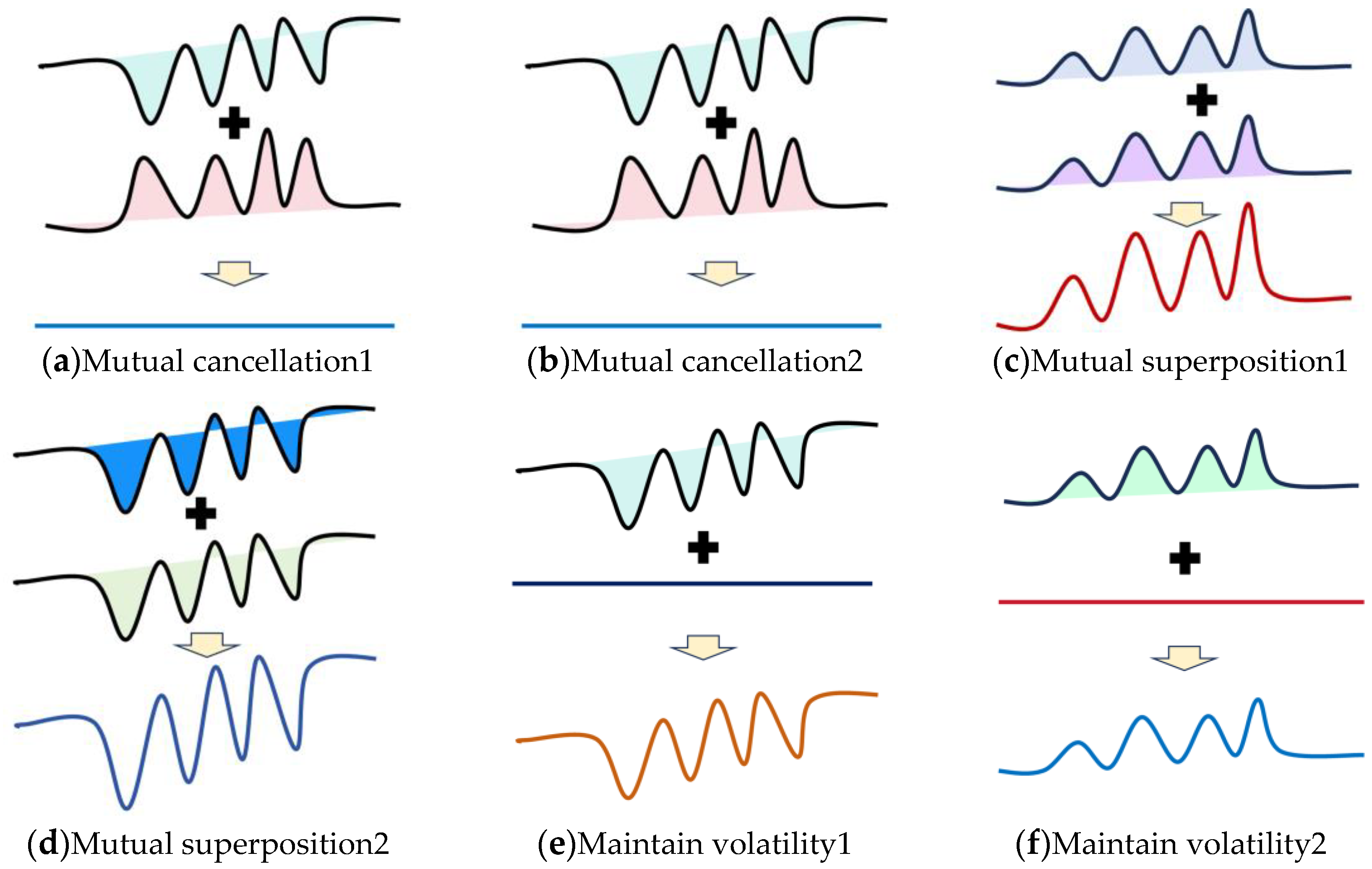
Figure 1. Smoothing effect of series with different levels of volatility after superposition.
Electronics 14 03641 g001
Figure 2. Improved fluctuation-smoothing loss function.
Electronics 14 03641 g002
Figure 3. The network architecture of STHDGCN-BITCN.
Electronics 14 03641 g003
Figure 4. Overall research technology framework.
Electronics 14 03641 g004
Figure 5. Prediction curves of different modeling methods corresponding to different models.
Electronics 14 03641 g005aElectronics 14 03641 g005b
Figure 6. Cluster dynamic division results for three different cluster dynamic division mechanisms corresponding to a certain moment of time.
Electronics 14 03641 g006aElectronics 14 03641 g006b
Figure 7. Prediction error assessment metrics for each graphical model under different cluster dynamic division mechanisms.
Electronics 14 03641 g007aElectronics 14 03641 g007b
Figure 8. Prediction curves for different cluster dynamic division mechanisms corresponding to representative time periods for different prediction models.
Electronics 14 03641 g008aElectronics 14 03641 g008b
Figure 9. Prediction error distribution for different cluster dynamic division mechanisms corresponding to representative time periods for different prediction models.
Electronics 14 03641 g009
Figure 10. Error distribution of daily series corresponding to different modeling approaches.
Electronics 14 03641 g010aElectronics 14 03641 g010b
Figure 11. Error distribution of hourly series corresponding to different modeling approaches.
Electronics 14 03641 g011aElectronics 14 03641 g011b
Table 1. Geographic location information of PV stations in the PV cluster.
Information ItemsValue
Longitude interval[E 96°10′~E 102°12′]
Latitude interval[N 37°28′~N 40°52′]
Number of PV stations30
Rated capacity1500 MW
Table 2. Indicators of prediction error assessment for different modeling approaches corresponding to different prediction models (specific methods can be found in [15,18]).
Modeling MethodsIndexMLRRFBPBITCNTransformer
Cumulative methodNRMSE0.11580.11190.10740.09230.0922
NMAE0.06330.05870.05880.04900.0491
R20.46090.58210.56780.73130.7402
Holistic approachNRMSE0.11320.08660.10740.07830.0895
NMAE0.06030.04610.05880.04050.0473
R20.58090.77650.56780.87280.7570
Statistical upscalingNRMSE0.13220.11450.12440.08550.1035
NMAE0.07300.06280.06870.04430.0556
R20.13350.46000.28430.82110.6159
Cluster static divisionNRMSE0.10050.09580.09170.07470.0823
NMAE0.05420.05210.04970.03910.0426
R20.66450.76660.73990.85940.8121
Table 3. Volatility of sub-cluster power in three clustering scenarios corresponding to three clustering models at different clustering distances.
Clustering ModelClustering DistanceSub-Cluster-ISub-Cluster-IISub-Cluster-III
DAEGC [77]Kullback–Leibler divergence0.36590.78640.8841
Spectral clusteringCorrelation coefficient0.45620.63940.8772
Sample entropy0.35220.78820.8589
IDis0.37210.38440.3921
k-meansCorrelation coefficient0.45140.64540.8769
Sample entropy0.35340.78780.8596
IDis0.37040.38540.3901
Table 4. Error assessment metrics corresponding to different models under different similarity classification bases.
Cluster Division MethodsIndexMLRRFBPBITCNTransformer
Correlation coefficientNRMSE0.11400.10250.11040.08280.0842
NMAE0.05210.03830.04920.04610.0470
R20.66600.83420.71410.78440.7736
Sample entropy similarityNRMSE0.10850.11090.10700.07540.0768
NMAE0.04740.04760.04620.04180.0427
R20.74570.83710.77430.83450.8255
Smoothing effect functionNRMSE0.07230.08600.08860.06650.0671
NMAE0.03780.04300.04750.03740.0378
R20.83380.86620.79490.88010.8774
Table 5. Comparison of modeling time cost of different modeling approaches in different sessions.
Modeling SessionCumulative Method (s)Holistic Approach (s)Statistical Upscaling (s)Cluster Static Division (s)Proposed (s)
Cluster division###6.7451279.9040
Looking for nominal PV stations##30.2451##
Constructed graph structure####21.0461
Training models36,045.2377123.4501123.6553740.7201302.4566
Prediction70.63802.054510.150314.12766.5741
Total36,115.8757125.5046164.0507761.5928609.9808
Note: “#” indicates that it is not applicable and that the time consumption of the different modeling methods at different sessions is the average of multiple models. (Specific methods can be found in [15,18]).
Disclaimer/Publisher’s Note: The statements, opinions and data contained in all publications are solely those of the individual author(s) and contributor(s) and not of MDPI and/or the editor(s). MDPI and/or the editor(s) disclaim responsibility for any injury to people or property resulting from any ideas, methods, instructions or products referred to in the content.