Article

Parallelization of the Koopman Operator Based on CUDA and Its Application in Multidimensional Flight Trajectory Prediction

School of Computer Science and Artificial Intelligence, Civil Aviation Flight University of China, Guanghan 618307, China
*
Author to whom correspondence should be addressed.
Electronics 2025, 14(18), 3609; https://doi.org/10.3390/electronics14183609
Submission received: 29 July 2025 / Revised: 5 September 2025 / Accepted: 8 September 2025 / Published: 11 September 2025

Abstract

This paper introduces a parallelized approach to reconstruct Koopman computational graphs from the perspective of parallel computing to address the computational efficiency bottleneck in approximating Koopman operators within high-dimensional spaces. We propose the KPA (Koopman Parallel Accelerator), a parallelized algorithm that restructures the Koopman computational workflow to transform sequential time-step computations into parallel tasks. KPA leverages GPU parallelism to improve execution efficiency without compromising model accuracy. To validate the algorithm’s effectiveness, we apply KPA to a flight trajectory prediction scenario based on the Koopman operator. Within the CUDA kernel implementation of KPA, several optimization techniques—such as shared memory, tiling, double buffering, and data prefetching—are employed. We compare our implementation against two baselines: the original Koopman neural operator for trajectory prediction implemented in TensorFlow (TF-baseline) and its XLA-compiled variant (TF-XLA). The experimental results demonstrate that KPA achieves a 2.47× speed up over TF-baseline and a 1.09× improvement over TF-XLA when predicting a 1422-dimensional flight trajectory. Additionally, an ablation study on block size and the number of streaming multiprocessors (SMs) reveals that the best performance is obtained with the block size of 16 × 16 and SM = 8. The results demonstrate that KPA can significantly accelerate Koopman operator computations, making it suitable for high-dimensional, large-scale, or real-time applications.

1. Introduction

The evolution of nonlinear dynamical systems with unpredictable behavior reflects many real-world phenomena upon which humans rely, such as atmospheric and climate systems, fluid dynamics, mechanical vibrations, and economic market models. In recent years, scholars across various disciplines have been exploring efficient and interpretable methods to understand these complex dynamical behaviors. The Koopman operator theory (KOT) emerged as a key analytical tool among others to cope with nonlinear dynamical systems. Originally introduced in Koopman’s early work [1], the theory provides a framework for analyzing finite-dimensional nonlinear differential equations by mapping the system states into a high-dimensional observable space, where the system’s nonlinear evolution can be approximated as linear.
Although the Koopman operator can “linearize” a nonlinear system, it is inherently an infinite-dimensional linear operator, which poses significant challenges for practical descriptions and applications [2]. Nevertheless, due to the absence of practical modeling methods and the difficulty of handling high-dimensional data, the Koopman framework saw limited uses in numerical computation for several decades despite its theoretical appeals. In the past decade, interest in the theory increased [3,4]. Schmid introduced the Dynamic Mode Decomposition (DMD), which provided a finite-dimensional approximation of the Koopman operator by constructing a matrix from pairs of state observations [5]. Since then, a range of data-driven approximation techniques have been developed for the Koopman operator [6] (e.g., EDMD, KDMD). The powerful characterization capability of deep learning has enabled researchers to adopt nonlinear functions—particularly neural networks—to construct observable functions. By training neural networks to learn nonlinear mappings that project system states into an approximate Koopman observable space, researchers can obtain an approximate linear representation of the Koopman operator without explicit definitions of basis functions (e.g., DeepKoopman [7], Autoencoder-Koopman [8]).
While deep learning has enhanced the Koopman framework’s ability to model complex dynamical behaviors, computational efficiency remains a bottleneck during training. As the dimensionality of states and observables increases, solving the Koopman operator turns into a large-scale least squares problem. Its closed-form solution often relies on the pseudo-inverse computation [9], which can be computationally expensive. Moreover, the solving process involves numerous intermediate matrix constructions and data transformations that are inherently sequential, exacerbating the consumption of computational resources, particularly in large-scale batches and high-dimensional spaces. Since the Koopman operator is non-differentiable, it cannot be incorporated into the automatic differentiation graph of deep learning frameworks directly, further limiting its scalability and performance in large-scale modeling tasks.
The rapid development of modern GPUs has continuously optimized and accelerated the computational efficiency of deep learning. According to NVIDIA’s official documentation, a range of GPU acceleration techniques—such as batch SVD in cuSOLVER [10] and the optimized GEMM kernel in cuBLAS [11]—significantly improve the efficiency of linear algebra operations in deep learning models. However, these methods are not designed for end-to-end Koopman computational workflows, as the state pairs required for computing the Koopman operator are consecutive, resulting in inherently sequential execution of the corresponding computational processes. Even when acceleration techniques are employed to speed up individual steps, this sequential nature remains inefficient as data dimensionality increases. In our subsequent optimization of the Koopman algorithm, we will not only utilize these interface tools to perform standard matrix operations but also reconstruct the Koopman workflow by decoupling its dependencies and exploring opportunities for parallel execution, thereby maximizing GPU resource utilization.
To address these issues, this paper proposes a CUDA-based Koopman Parallel Accelerator (KPA) algorithm. This algorithm is designed to accelerate Koopman operator computation on GPU, significantly improving efficiency and real-time performance without altering the model architecture or prediction accuracy. It also offers strong generalizability and ease of deployment. To validate the proposed algorithm, we apply it to the multidimensional flight trajectory prediction (MFTP) task. Specifically, we integrate the KPA algorithm into the FlightKoopman model based on the works in [12] and implement a GPU-parallelized version of the Koopman solver.
The main contributions of this paper are as follows:
  • We propose a GPU-based parallel optimization method for computing Koopman operators, addressing the computational bottlenecks associated with high-dimensional state spaces.
  • We implement a general-purpose module interface that supports multiple Koopman solving strategies, providing good scalability.
  • We verify the acceleration performance and prediction stability of the proposed method on the MFTP task. The experimental results demonstrate significant improvements in training efficiency.
This paper is organized as follows: Section 2 introduces the Koopman operator theory; Section 3 presents the design and implementation of the KPA algorithm; Section 4 details the experimental setups and results for the MFTP task; and Section 5 concludes this paper and outlines directions for future works.

2. Preliminaries

2.1. Koopman Operator

The Koopman operator provides a linear representation of a nonlinear dynamical system by acting on a function of the system’s state (the observation), rather than on the state itself. This approach preserves the essential characteristics of the system’s dynamics while enabling prediction or detection tasks using the analytical tools of linear systems. Such linearization-based techniques are valuable in many dynamical systems. In aerospace applications, for example, they are widely used in flight control and management systems where accurate attitude estimation is essential [13]. These techniques provide a practical approach to handling nonlinear dynamics in real time. Their importance in engineering is further highlighted by recent studies showing that internal resonance mechanisms can be exploited to achieve synchronous broadband vibration mitigation and energy harvesting [14].
For a discrete-time nonlinear system with state x t R n , the evolution is governed by an unknown nonlinear function:
x t + 1 = f ( x t )
where f is the state transition function of the nonlinear system. By applying the infinite-dimensional Koopman operator K , the system can be represented as a linear evolution in a high-dimensional feature space. Rather than directly simulating f ( · ) , the Koopman framework seeks a mapping Φ : R n R N that projects the original state variables into a high-dimensional space where the evolution becomes approximately linear:
Φ ( f ( x t ) ) = K Φ ( x t )
Hence, the Koopman operator acting on the observation function F is given by the following:
Φ ( x t + 1 ) = K Φ ( x t )
This implies that the linear operator K can propagate observations at the current time step linearly to the next time step, and  K can be applied iteratively to predict future observations over the next t steps.
Since the Koopman operator is fundamentally a linear operator acting on an infinite-dimensional function space, it is not possible to store or manipulate its accurate representation using finite computational resources. Therefore, practical applications of the Koopman framework require finite-dimensional approximations. Therefore, the subsequent studies in this paper and practical applications adopt approximate Koopman operators, which are finite-dimensional matrices designed to capture the dominant linear dynamics in a predefined or learned observable space. Classical methods such as Dynamic Mode Decomposition (DMD) and its variants offer viable linear algebraic frameworks to approximate the Koopman operator. However, these approaches involve the eigen decomposition of potentially non-symmetric matrices, which impedes efficient parallelization on GPU.
To overcome this obstacle, we focus on a data-driven approach to construct finite-dimensional approximations of the Koopman operator by learning appropriate observable functions directly from the data. With this method, it captures the system’s approximate linear evolution in a learned feature space. In the following section, we elaborate on the design and training of neural network architectures that enable efficient approximation of the Koopman operator.

2.2. Koopman Training

Currently, many researchers have combined the theory of Koopman operators with neural network methods to perform some work on modeling nonlinear systems, such as [15,16]. Building on this idea, the Koopman neural operator is essentially a neural network-based implementation of the approximate Koopman operator, achieving the finite-dimensional approximation introduced earlier. Unlike traditional methods, it learns the observable mapping from data rather than relying on manual specification. In the framework based on deep Koopman neural operators (DeepKONet structure), in order to construct infinite-dimensional Koopman operator approximation K R n × n , the neural network encoder is combined with the linear operator for analytical estimation [17]. The evolution process of the nonlinear system is approximated as a linear system by constructing the observation function that maps the original state to the high-dimensional observation space through deep learning.
The entire training model framework consists of three main components: the encoder, which extracts features from the original data to construct the observation function; the Koopman solver, which uses the data matrix generated by the encoder to perform a linear transformation that approximates the Koopman operator; and the decoder, which maps the state g t in the Koopman observation space back to the original trajectory space to obtain the future state data. The overall structure is illustrated in Figure 1. The individual components of this framework are described in the following sections.
Encoder. The neural network is used to construct the observation function Θ : R n R N , which enables the projection of the input state x t R n to enter into a lifted observable space, obtaining the high-dimensional eigenvector g t (Equation (4)),
g t = Θ ( x t )
and constructing the decomposition of g t into two data matrices:
X = [ g 0 , g 1 , . . . , g T 1 ]
Y = [ g 1 , g 2 , . . . , g T ]
Next, the operator K needs to be computed such that the state updated in the Koopman space can be expressed as a linear relation, i.e.,
K g t = g t + 1
Koopman solver. In order to solve K, a least squares approach is used:
min K Y X K F 2
In order to avoid the high memory and numerical stability problems associated with the direct use of X and Y, we adopt an equivalent approach by constructing the covariance matrices G = X T X and A = X T Y . The matrix G captures the autocorrelation between consecutive observations, reflecting the stability of the observation (Equation (9)). The matrix A encodes the stepwise relationship between neighboring observations, thus reflecting the dynamic evolution of the state (Equation (10)).
G = 1 n t = 1 n g t T g t
A = 1 n t = 1 n g t T g t + 1
Finally, the Koopman operator is given by Equation (11) within this framework,
K G A
We support two solver variants:
  • The full pseudo-inverse, which is computed using the full singular value decomposition (SVD) when solving for the pseudo-inverse of G.
  • The truncated SVD, retaining only the top r singularities of G to improve the stability and control of the model’scapability. That is,
K G r A
Decoder. The role of the decoder is to map the state g t in the Koopman observation space back to the original trajectory space, thereby recovering the future state from the current observation through iterative computation:
g t + 1 = K g t , g t + 2 = K g t + 1 , , g t + T = K T g t
Eventually, the predicted observations are transformed back into the original state space by the decoder (Equation (13)),
x t + T = Ψ ( g t + T )
Throughout the framework, the Koopman operator is not treated as a learnable parameter. Instead, it is re-estimated in each training iteration based on the current batch of data. The encoder and decoder are trained jointly via backpropagation, while the Koopman operator estimation is decoupled from this process. This separation not only simplifies model training but also enables independent optimization of the estimation step.
Although the Koopman operator theory effectively balances physical interpretability with data adaptability when combined with data-driven approaches, its serial computational nature leads to increased complexity in high-dimensional feature spaces due to dense matrix operations. To address this challenge, a parallel optimization algorithm that maps the core serial operations of Koopman operator estimation onto GPU-parallel architecture is introduced. This mapping is achieved through techniques such as operation chunking, memory access optimization, and mixed-precision computation to ensure efficient acceleration.

3. Algorithm Design

In this section, we first analyze the computational complexity and data dependencies involved in Koopman operator estimation. Based on this analysis, we propose a parallel computing optimization algorithm—KPA (Koopman Parallel Accelerator). KPA improves the execution efficiency of Koopman operator computation through task decomposition, hierarchical task assignment, memory layout reconfiguration, and optimization of computation strategies.
Given that application-specific Koopman solvers may differ—for example, someone prefers the accurate reconstruction using a full pseudo-inverse, while others adopt truncated SVD to enhance stability or enable compression—these variations nevertheless share a significant portion of input matrices and intermediate computations. Therefore, KPA focuses on optimizing the core low-level operations common to Koopman estimation while also providing modular interface support for easy extensibility and strategy switching.

3.1. Computational Complexity Analysis and Optimization Motivation

Before optimizing computations of the Koopman neural operator, it is necessary to theoretically analyze its computational complexity and identify the primary bottlenecks. This section first establishes a computational complexity model for the Koopman operator by quantifying overheads of various operators. The key computation-intensive components are identified, and a directed acyclic graph (DAG) model to analyze the dependencies among operators [18] is constructed. Through this analysis, the main data flow patterns are identified, thereby providing a theoretical basis for subsequent parallel algorithm design and indicating potential optimization directions.

3.1.1. Identification of Computation-Intensive Regions and Complexity Modeling

In the Koopman operator estimation process, the training data typically consist of a set of state transition observation pairs { x i , y i }, where x i R d denotes the state of the system at the i-th sampling point, and  y i R d represents the observation of the next state. Each observation pair is associated with a corresponding feature extraction and matrix operation. As a result, each training iteration involves multiple small-scale matrix multiplications, with a floating-point operation time complexity of O m n N 2 , where N is the dimensionality of the Koopman feature space, n is the number of observation pairs per sample, and m is the batch size. However, the subsequent pseudo-inverse operation depends on SVD, which has a complexity of O m N 3 . Additionally, the computation of the approximate Koopman operator K also incurs a complexity of O m N 3 due to the matrix multiplications involved.
Overall, solving the Koopman operator is computation-intensive, especially in practical scenarios where input data often take the form of dense matrices, placing significant demands on memory bandwidth and computational efficiency. This fact underscores the necessity of algorithmic reconfiguration and parallel optimization to improve the performance of Koopman operator computation.

3.1.2. Operator Dependency DAG Modeling

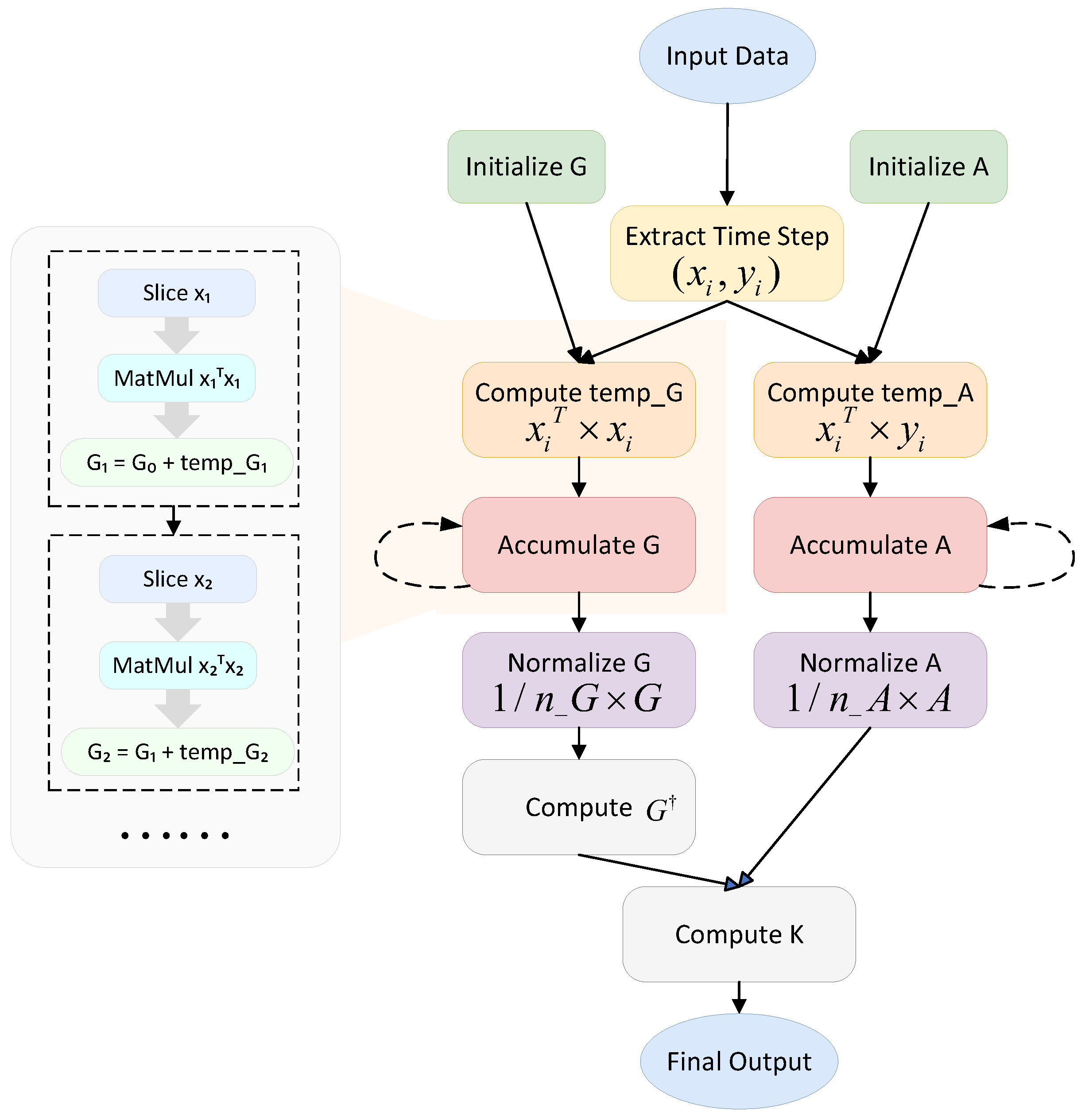
Through the performance analysis tool Profiler, several core operators from the network layer containing the Koopman neural operator were extracted, as outlined in Table 1. By analyzing the fine-grained dependencies of these operators, a DAG (directed acyclic graph) is constructed in Figure 2.
The core computational flow of the Koopman algorithm begins with a slicing operation on the input data. A set of grouped state transition observation pairs { x i , y i } is extracted from the high-dimensional input tensor via indexing. This is followed by matrix multiplication operations that produce intermediate variables, temp_G and temp_A, which are then accumulated globally. This process is implemented through an explicit loop over the observation pair indices, where each iteration depends strictly on the accumulated results from the previous step, forming a strong sequential dependency chain. After all observation pairs are processed through the sequence of Slice → MatMul → Add, the accumulated G and A matrices are normalized via scalar multiplication (ScalarMul), and a pseudo-inverse of G is computed to obtain the Koopman operator K, which is subsequently applied to the input data to generate predictions or reconstructions. The primary computational bottleneck in this pipeline lies in the serial dependencies during the loop-based accumulation phase: each iteration must wait for the completion of the previous one. These procedures severely limit the utilization of GPU computational resources, resulting in suboptimal performance.
When examining the fine-grained dependencies within each loop iteration, taking the computation of G as an example, the accumulation process can be decomposed into three steps: (1) the input tensor is sliced to extract the state x i from the current observation pair; (2) a temporary matrix is computed temp _ G i = x i T x i ; and (3) this intermediate result is accumulated into the global matrix G. Due to the strict dependency of each accumulation step on the result of the previous one (i.e., G i depends on G i 1 ), a chained data dependency is formed. As a result, computations inside the loop cannot be parallelized. Moreover, the accumulation phase involves frequent global memory reads and writes, which significantly increases memory access latency and further degrades computational efficiency.

3.2. Design of Parallel Algorithms for the Koopman Operator

Through the analysis of operator dependencies, we found that the computation of the Koopman operator exhibits strong sequential dependencies among operators. Therefore, it is necessary to restructure the overall computation graph, to unroll loops, transforming them into batch operations, and fully utilize shared memory in GPU memory while avoiding memory access conflicts during data transmission.

3.2.1. Multi-Granularity Parallel Task Decomposition

KPA decomposes and refines multiple computational tasks in Koopman operator estimation, enabling end-to-end parallelization—from data loading to result output—through multi-level task partitioning and coordinated scheduling of hardware resources. The decomposed tasks are mapped to independent CUDA cores and executed in parallel streams to fully exploit the concurrency of GPU. To structure the overall KPA framework, we adopt a hybrid static–dynamic execution model, in which CUDA Streams provide a dynamic task scheduling environment [19], while CUDA Graphs are used to statically optimize task execution and reduce kernel launch overhead.
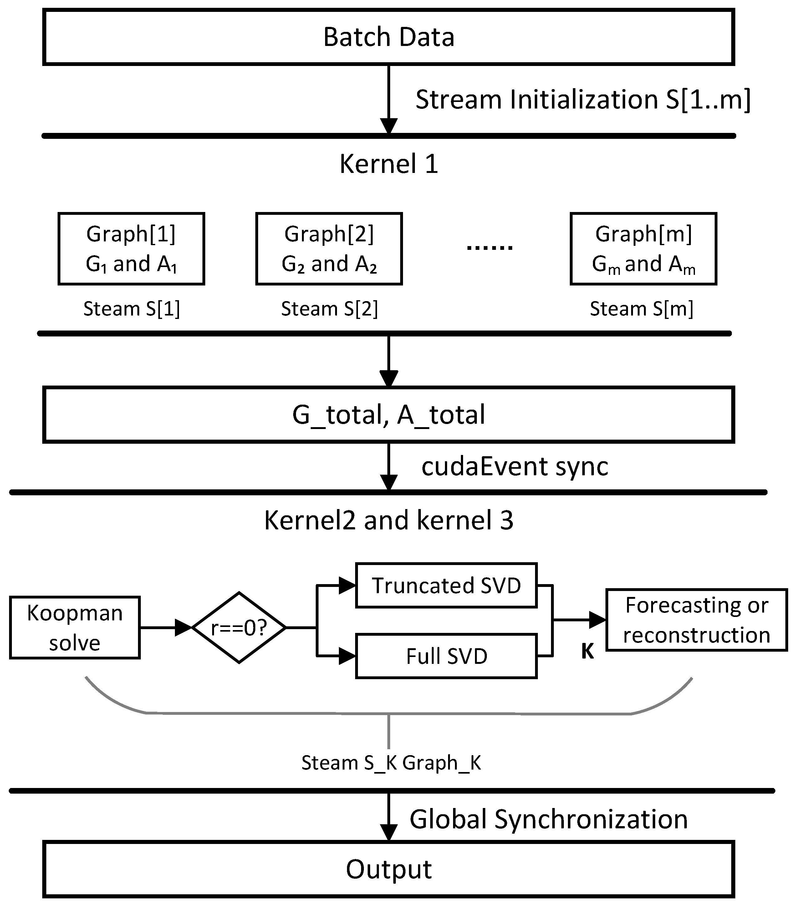
The core task decomposition logic of the KPA algorithm is illustrated in Algorithm 1, whose computational flow is depicted in Figure 3:
Algorithm 1 KPA Framework
  1:
Input: tensor X R B × T × N , Number of CUDA streams m, Tile size N s
  2:
Output: Predicted or reconstructed results Y
  3:
Initialize CUDA Streams { S 1 , , S m } for G/A computation
  4:
for each stream S i  do
  5:
      Launch Kernel 1 in S i to compute G i = x t x t , A i = x t x t + 1
  6:
      Capture CUDA Graph G r a p h i for Kernel 1 (computing G i and A i )
  7:
      Launch graph G i on S i for sub-batch X i
  8:
      Record event_GA at end of each stream S i
  9:
end for
10:
Create a dedicated stream S K for Koopman solving and prediction
11:
Capture CUDA Graph G r a p h K for Kernel 2 and 3
12:
In  S K :
13:
    Wait for all event_GA
14:
    Aggregate G and A from all streams
15:
if  r = = 0  then
16:
          Launch Kernel 2 using full SVD (Moore-Penrose pseudo inverse)
17:
else
18:
          Launch Kernel 2 using truncated SVD (retain top r modes)
19:
end if
20:
    Launch Kernel 3: compute Y = X K
21:
Copy Y from device to host memory
22:
Synchronize all streams
KPA initializes S CUDA Streams along with corresponding CUDA Graphs, where each stream launches a statically captured graph to minimize kernel launch overhead [20]. These streams asynchronously read data in batches from host memory to GPU global memory. Each stream processes its assigned batch of samples independently, executing the required computational kernels without inter-stream interference.
The number of streams S is typically determined in relation to the number of streaming multiprocessors (SMs) on the GPU, and in conjunction with the study by [21], it can be approximated by the following empirical formula (Equation (14)):
S = m i n 4 × n u m b e r o f S M s , 128
However, the optimal number of streams should be dynamically adjusted based on specific GPU hardware characteristics in practice—such as memory bandwidth and total number of SMs—as well as the computational load of the task. A common heuristic is setting S between one-half and one-quarter of the total number of SMs to achieve a balanced trade-off between parallel efficiency and memory contention.
Specifically, the Koopman operator solving process is divided into three distinct CUDA kernel functions:
  • Kernel 1: This computes the covariance matrices for multiple batches of input data and performs normalization of matrices G and A.
  • Kernel 2: The cuSOLVER library is employed to perform SVD and compute the pseudo-inverse of G, which is used to solve the Koopman operator K. Within this kernel function, KPA defines a unified solver interface that supports both full and truncated SVD strategies. If r = 0 , a full pseudo-inverse is computed by retaining all singular values. If  r > 0 , a truncated SVD is applied, in which only the top r dominant singular values and their corresponding singular vectors are preserved. The algorithm incorporates a lightweight branching mechanism to determine the execution path—full or truncated—based on the value of r. This design avoids redundant memory accesses and the unnecessary duplication of intermediate results, thereby improving overall computational efficiency.
  • Kernel 3: This applies the estimated Koopman operator K to the input data to generate prediction or reconstruction results.
To improve efficiency, the fixed computational flows of these kernels are encapsulated using the CUDA Graph static execution mechanism. This allows for each stream to capture and execute its own CUDA Graph independently, enabling intra-stream task sequences to be statically optimized. Additionally, inter-stream coordination is achieved through CUDA event synchronization (i.e., cudaEvent), ensuring proper execution order across different graph instances. Considering that the pseudo-inverse computation typically has higher time complexity than the covariance matrix operations, we do not encapsulate the entire solving process into a single static graph. Instead, multiple streams are used to independently handle the normalization and accumulation of G and A matrices across batches. Once this stage is completed, its results are passed to a dedicated stream that performs the pseudo-inverse computation. The final prediction or reconstruction results are then computed subsequently.

3.2.2. Memory Partitioning and Access Optimization

In Algorithm 1, three kernel functions are launched to accomplish the parallel computation of tensors G and A, the asynchronous computation of the pseudo-inverse matrix, and the prediction. According to the mathematical principle of matrix multiplication given in Equation (15), the computation requires multiplying corresponding row and column elements of two matrices and summing the results [22]. If all data are stored in global memory during computation, frequent global memory access will become the performance bottleneck. Therefore, memory partitioning and access optimization are necessary to reduce the number of global memory accesses and improve computational efficiency. This subsection provides a detailed discussion of the specific optimization strategies for the kernel functions in Algorithm 1 of the KPA framework.
c i j = n k = 1 a i k b k j
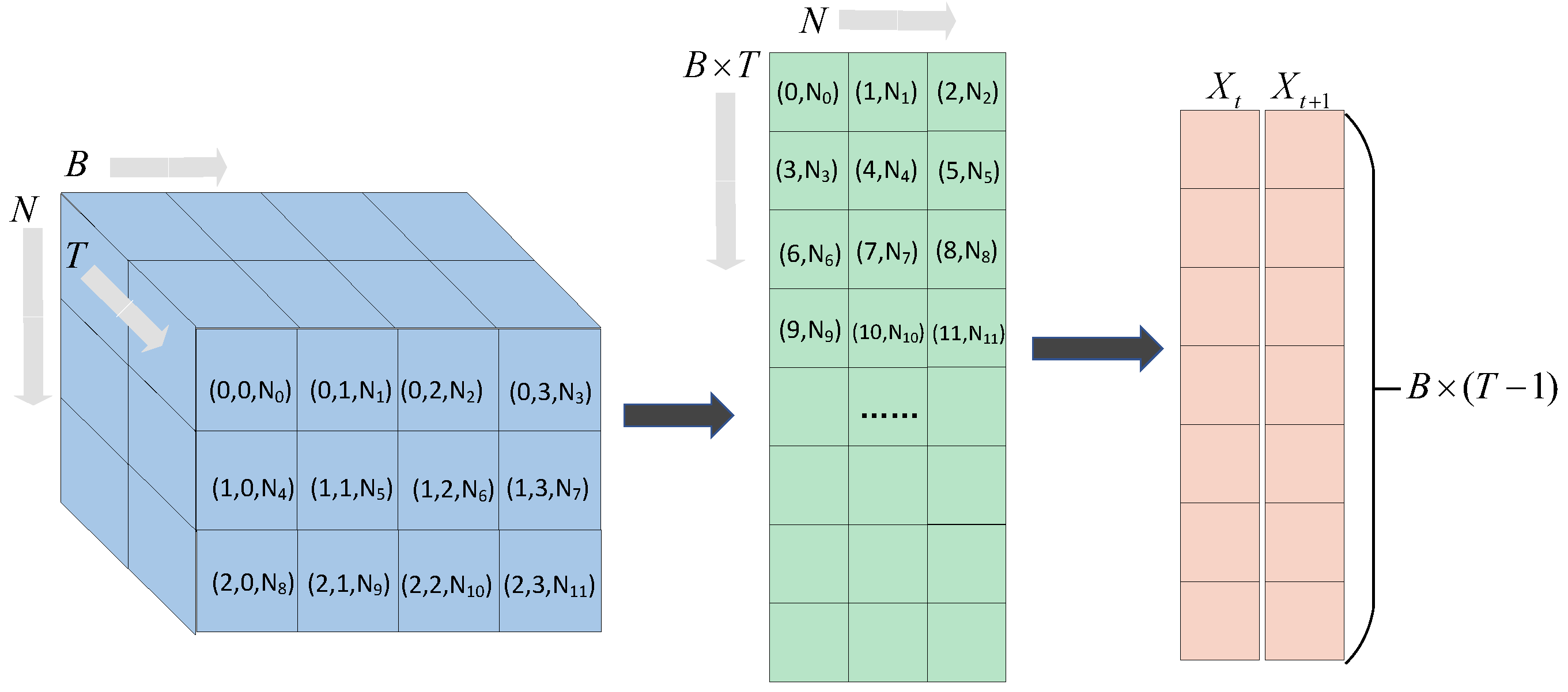
Dimension reorganization. In various experiments containing the Koopman operator, the volume of data is typically large. The input tensor X is generally structured as a three-dimensional array ( B , T , N ) , where B denotes the batch size, T the sequence length (or observation index length), and N the feature dimension. During computation, a set of state-shifted observation pairs { x i , y i x i , y i } , i [ 0 , T 1 ] , y i = x i + 1 , is extracted from the input data. Each observation in each batch is in the form of ( T , N ) , which is used to construct the covariance matrices G and A (each with form of ( N , N ) at index i). As shown in Equations (9) and (10), although G and A have different physical interpretations, their mathematical forms are computed in a very similar manner, relying solely on the current state observation and the subsequent state observation. Moreover, computations across different observation pairs are completely independent.
It is worth noting that the dimensional reorganization strategy we adopt does not alter the original data in terms of dimensionality; rather, it is merely a scheme for restructuring the indices of data tensors to achieve efficient memory access, rather than expanding or compressing the original feature space. This approach does not change the inherent feature dimension N of the state vector; instead, it is purely an optimization of memory layout aimed at maximizing coalesced memory access and kernel parallelism during matrix computations.
In order to optimize the computational efficiency and make full use of the parallel computing power of CUDA GPU, we adopt the dimension reorganization strategy, as illustrated in Figure 4, upon the related correlation matrix. Specifically, we merge the batch dimension B and the sequence dimension T into a unified observation index t and reorganize the data along row–column indices to form a two-dimensional input X R ( B × T ) × N , where each row corresponds to a state vector ( x t ) . Subsequently, B × ( T 1 ) continuous state observation pairs { x t , y t } are extracted via a sliding window y t = x t + 1 . These continuous state pairs are then reorganized into two two-dimensional matrices X t and X t + 1 , both with the form of ( B × ( T 1 ) ) × N .
Memory Partitioning. Based on the dimension reorganization, we adopt a chunked parallel computing strategy to divide the large matrix computation task into smaller, parallel-executed sub-tasks. Since the feature dimension N is typically large, it is partitioned into N s × N s sub-blocks. The choice of N s is determined by the GPU hardware architecture and the feature dimension [23], whose common values are 16, 32, 128, or 256. Each thread block is assigned to process one sub-block identified by a 2D thread grid index ( i , j ) , where i = N / N s , j = N / N s .
KPA enables S CUDA Streams and distributes the batch dimension samples in parallel across multiple CUDA Streams. Each stream processes approximately B s = B × ( T 1 ) / S samples. On the basis of this chunking strategy, the corresponding thread model is organized within CUDA. During the Kernel 1 phase, the thread blocks are designed as two-dimensional blocks with size N s × N s , while the grid is configured as a three-dimensional structure ( N + b l o c k . x 1 b l o c k . x , N + b l o c k . x 1 b l o c k . x , B * ( T 1 ) S ). The x and y dimensions manage sub-blocks, while the z dimension handles sample blocks.
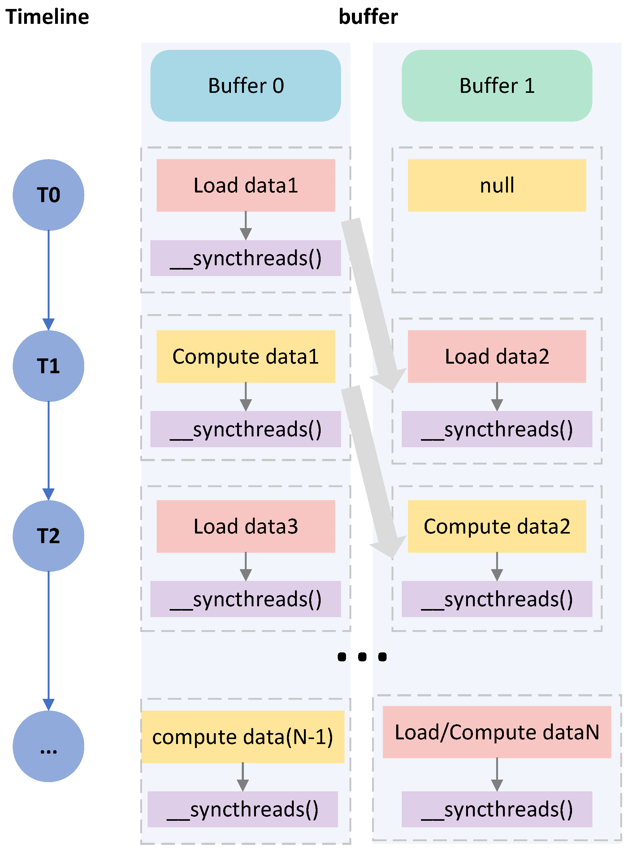
Access Optimization. To minimize unnecessary overhead caused by frequent global memory accesses during computation and to reduce data loading latency, we implement a sliding window mechanism [24] in shared memory using a double-buffering technique [25]. In this regard, a small region of GPU shared memory is allocated as a cache for read operations. It is organized into two separate buffers to support the double-buffering mechanism. Each thread block utilizes shared memory to load data from two consecutive observation pairs: one buffer holds the data for the current computation, while the other preloads the next set of data. Buffer switching is controlled via conditional branching combined with CUDA’s __syncthreads() synchronization primitive. When computation units process the current sub-block, the next sub-block of data is preloaded into shared memory at the same time, thereby improving memory access efficiency and overall computational throughput. Specifically, the cur buffer and the next buffer alternate roles in each iteration. The first state, i = 0 , is preloaded into the cur buffer before entering the first loop. Subsequently, state i = i + 1 can be loaded into the next buffer while buf[0] is being processed. This process continues iteratively, with each computation performed on the cur buffer, followed by synchronization using __syncthreads(), and then a swap of the buffer indices to safely reuse the preloaded data. This mechanism ensures that no thread reads stale data or overwrites data currently in use, thereby maintaining the correctness of concurrent memory accesses. The procedure is illustrated in Algorithm 2 (lines 9 to 20) and further clarified in Figure 5. Each time data are processed and the next state is loaded, synchronization occurs. Although synchronization introduces some time overhead, the double-buffer approach significantly reduces idle time compared with a single-buffer approach, where computation must pause while waiting for new data to be loaded.
In CUDA, a thread is the smallest unit for executing computational tasks, and 32 threads are grouped into a warp to perform computations. The shared memory is typically divided into 32 independent storage banks. Since each shared memory bank can only handle one access request at a time, conflicts occur when multiple threads within the same warp access different addresses within the same bank simultaneously [26]. To mitigate this issue, when allocating shared memory, an extra element is added to the shared memory size computed based on the actual feature count. This adjustment offsets the access pattern by shifting the starting position of each row, ensuring that consecutive row accesses are distributed across different banks. Furthermore, considering the case where the feature dimension is not an integer multiple of the block size, appropriate padding is required for memory alignment. This ensures that each block processes a complete segment of data, avoiding complex boundary condition checks.
Algorithm 2 KPA—Parallel Computation of G and A with Sliding Window and Double Buffer.
  1:
Input: Batch data X R B × T × N , Block size N s × N s
  2:
Output: Global matrices G, A R N × N
  3:
G 0 ; A 0       # Initialize global matrices
  4:
__shared__ buf[2][N_s][N_s+1]       # Double buffer with bank padding
  5:
c u r 0 ; n e x t 1       # Buffer index initialization
  6:
for each stream s in parallel do
  7:
      for each batch_idx in assigned_batches(s) do
  8:
            # Preload first observation into buf[cur]
  9:
            buf[cur]  X [ batch _ idx ] [ 0 ] [ : ]
10:
            for  t = 0 to T 2  do
11:
                 # Preload next observation into buf[next]
12:
                 buf[next]  X [ batch _ idx ] [ t + 1 ] [ : ]
13:
                 __syncthreads() # Ensure both buffers are ready
14:
                 # Compute contributions using buf[cur] and buf[next]
15:
                  Δ G block buf [ cur ] × buf [ cur ]
16:
                  Δ A block buf [ cur ] × buf [ next ]
17:
                 atomicAdd(G, Δ G block ); atomicAdd(A, Δ A block )
18:
                 __syncthreads() # Wait for all threads to finish accumulation
19:
                 # Swap buffers for next iteration
20:
                 swap(cur, next)
21:
            end for
22:
      end for
23:
end for
24:
G G / ( B × ( T 1 ) ) ; A A / ( B × ( T 1 ) )       # Normalize
Based on the above optimization strategy, KPA implements efficient parallel computation in Kernel 1. Specifically, the global matrices G and A and the shared memory double buffer are initialized first. Then, the double-buffer mechanism is used to asynchronously add in the consecutive state data, combined with the sliding window to complete the efficient scheduling of the data flow. Each state’s data are assigned to a different thread to complete the corresponding computation using the thread organization model. The results are stored into the buffer. The fully accumulated G and A are normalized until all thread blocks have completed the computation. The implementation flow of KPA is shown in Algorithm 2.
After the optimization of the KPA algorithm, the time complexity of Kernel 1 is O ( m n N / P ) , where m is the number of streams, n = B ( T 1 ) is the total number of observation pairs, N is the feature dimension, and P is the number of GPU threads × the number of streams (in parallel). Kernel 2 and Kernel 3, on the other hand, use the cuSolver library for pseudo-inverse solving and cuBLAS for efficient matrix multiplication of the prediction results, respectively.

4. Experiment and Analysis of the Results

In the previous sections, we analyzed the bottlenecks encountered in Koopman operator solving and designed the corresponding parallel optimization algorithm, KPA, which reconstructed the overall computational graph. In this section, to validate KPA’s function and efficiency, it is applied in the multidimensional flight trajectory prediction (MFTP) [27]. An MFTP model called FlightKoopman was proposed in [12], which used deep learning to construct an observation function that maps the original nonlinear states into a high-dimensional observable space. It leverages flight trajectory time-series data to approximate the linear Koopman operator.
Since the Koopman operator in this prediction model is not differentiable and is not updated via backpropagation, FlightKoopman is only partially GPU-accelerated. To be specific, the GPU acceleration of FlightKoopman is applied to the neural network training (e.g., training the observation function), while the data-intensive and time-consuming Koopman operator computation is not fully GPU-accelerated. Hence, this component does not make full use of GPU parallelism. To address this limitation, we separate the Koopman operator computation from the training graph and incorporate it into the model as an external module, thereby reducing prediction time and improving the overall efficiency.

4.1. Dataset and Experimental Environment

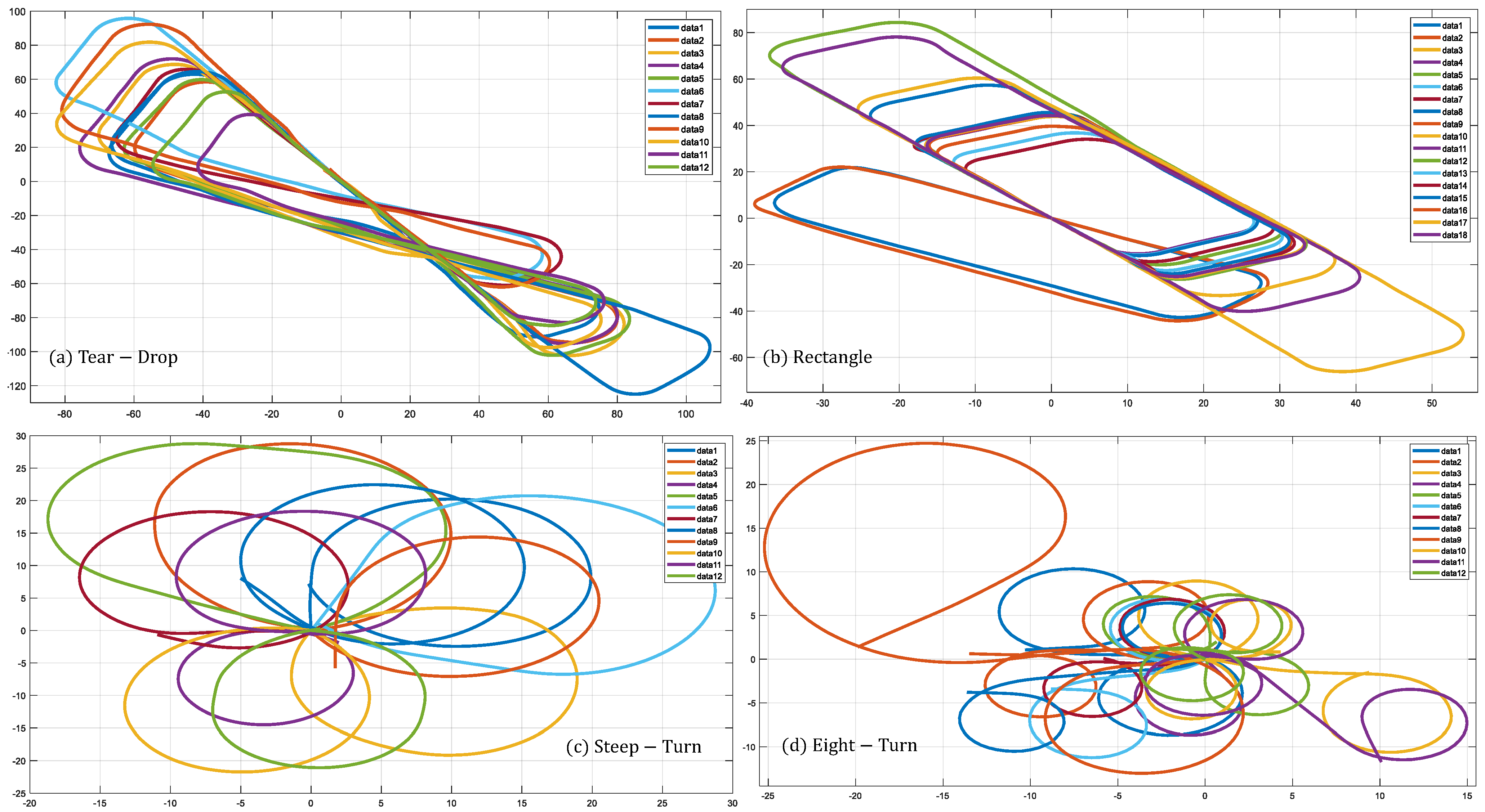
The dataset employed in this study consists of flight training data collected from real fixed-wing planes of the Civil Aviation Flight University of China (CAFUC). This dataset, referred to as the CAFUC dataset, records 41.6 h of flight data, comprising 64 parameters, 4 personal labels, and a total of 150,000 frames provided in CSV format [28]. Data of four types of training trajectories, the Tear-Drop, Rectangle, Steep-turn, and Eight-turn, which are shown in Figure 6, are used as samples in this study. Note that the data of Rectangle are formed from 18 trajectories, while the other three contain 12 trajectories. Additionally, this study makes use of two publicly available real-world benchmark datasets, the Exchange and Electricity. After preprocessing, the feature dimensionality of the CAFUC dataset increased from 12 to 1422, that of the Exchange [29] dataset expanded from 7 to 672, and the Electricity [30] dataset contains 1430 features.
The experimental hardware in this study is a server equipped with an NVIDIA GeForce RTX 3090 GPU (NVIDIA Corporation, Santa Clara, CA, USA), which supports 82 streaming multiprocessors. On the software level, the experiments are developed using CUDA Toolkit 12.2, integrating the cuBLAS and cuSOLVER mathematical libraries. The operating system is Ubuntu 22.04 LTS. Performance profiling and visualization are conducted using NVIDIA Nsight Systems 2023.3 and the CUDA Event API.

4.2. Evaluation Metrics

To evaluate the effectiveness of the CUDA-based parallel optimization scheme proposed in this study, time performance, resource efficiency, and accuracy assessment are selected as evaluation metrics. Our analysis focuses on the parallelization of the Koopman operator, which is essentially a non-microable computational module within the flight trajectory prediction model. To avoid the time-consuming overhead of forward propagation, backpropagation, and gradient updates associated with deep neural network training, the performance evaluation is restricted to the component of the model where the Koopman operator executes a single iteration. The measurements are averaged over 100 repeated runs to ensure stability and reliability of the results. The Table 2 presents the three categories of defined metrics: iteration time and speed up ratio are obtained by adding timers to the model, while throughput is measured using NVIDIA’s profiling tool Nsight Compute. For accuracy, we employ the absolute error formula to quantify the difference between methods.

4.3. Experimental Design

4.3.1. Benchmark Testing

To systematically evaluate the performance gains of the customized CUDA optimization, we select two baseline implementations: the original Koopman neural operator-based flight trajectory prediction model implemented using the TensorFlow framework (TF-Baseline) and an implementation optimized through XLA compilation (TF-XLA). All three experimental configurations are conducted using TensorFlow v2.15.0, CUDA v12.1, and cuDNN v8.9.1. Related notions and descriptions associated with experiments are listed in Table 3.
This experiment investigates the parallel optimization algorithm for the Koopman operator layer using CUDA, accompanied by a structural and code-level refactoring of the associated framework. Based on the DAG (directed acyclic graph) construction discussed in previous sections, operator dependencies were systematically identified, and corresponding operator-level parallelization strategies were developed to address specific computational challenges. The proposed KPA algorithm integrates various acceleration techniques, including shared memory double buffering, and memory tiling for matrix partitioning. During the data preprocessing stage, tens of thousands of trajectory samples underwent data cleaning, time-delay embedding, and Hankel matrix transformation, resulting in a flight trajectory dataset with 1422-dimensional features.
Specifically, based on real-world collected flight trajectory data, each raw trajectory sample consists of state vectors (e.g., latitude, longitude, altitude, velocity, and attitude parameters) with an original dimensionality of d o r i g = 12 . To approximate the Koopman space and capture temporal correlations, a time-delay embedding with a window size of ϵ + 1 is applied, resulting in a Hankel-structured representation of dimension d Hankel = ( ϵ + 1 ) × d orig . For instance, setting ϵ = 2 in the experiments yields d Hankel = 36 . Subsequently, to enhance the representation and construct a high-dimensional observable space, this representation is further extended by incorporating a second-order polynomial basis and a generalized observable library of Fourier terms, ultimately forming a high-dimensional vector of 1422 dimensions. For flight trajectory prediction tasks, the dataset was split into 80% for training and 20% for testing. As this study primarily focuses on the computational performance optimization of the Koopman operator, the emphasis was placed on the training dataset.
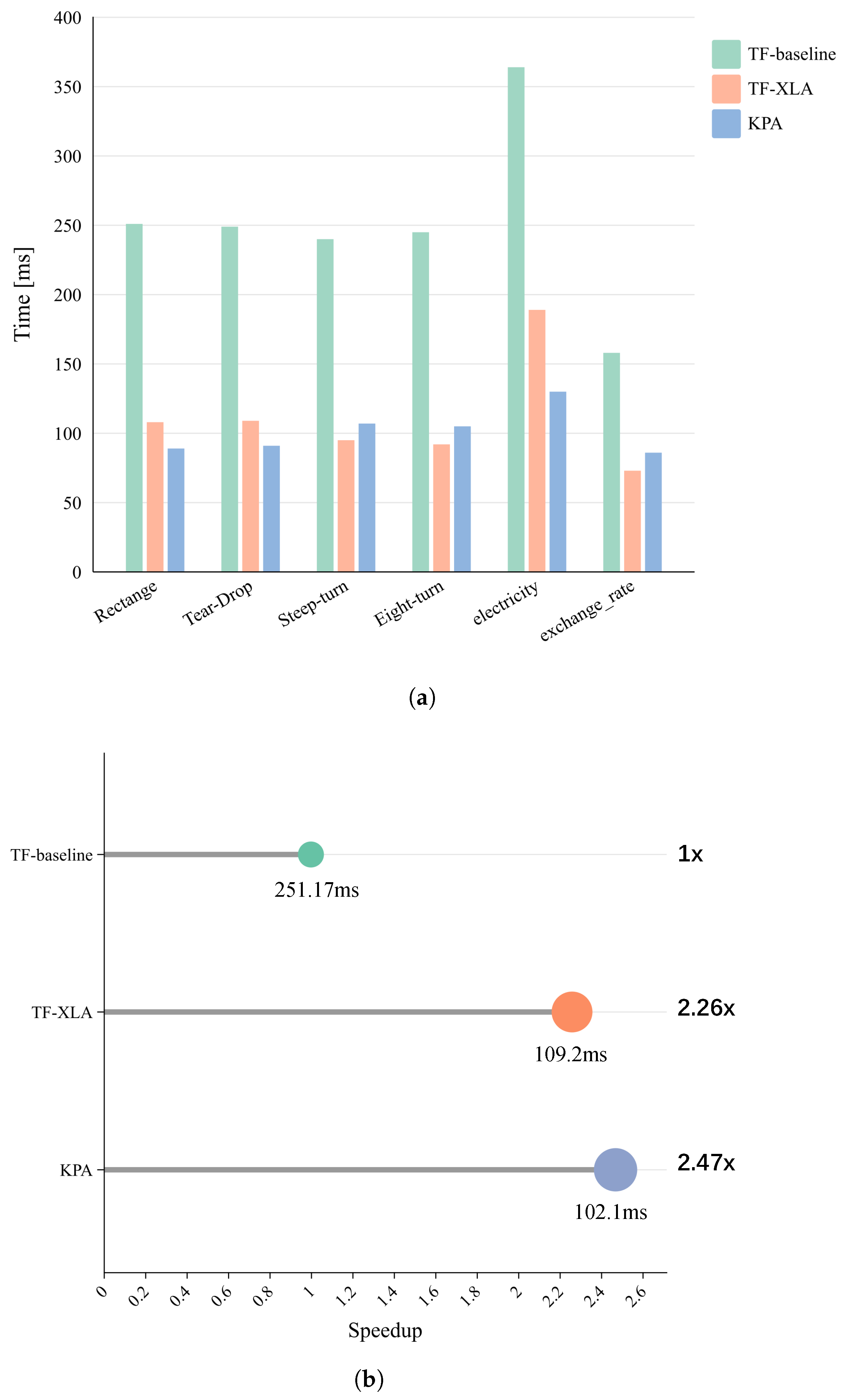
Figure 7a presents a performance comparison of execution time across three benchmark experiments. While the overall acceleration achieved by the KPA method slightly outperforms the other two approaches, the time performance of the Steep-turn, Eight-turn, and Exchange datasets showed marginally inferior iteration time performance compared to KPA. These three datasets have smaller data volumes and lower feature dimensions, indicating that the proposed KPA has greater efficiency gains when applied to larger-scale, higher-dimensional datasets.
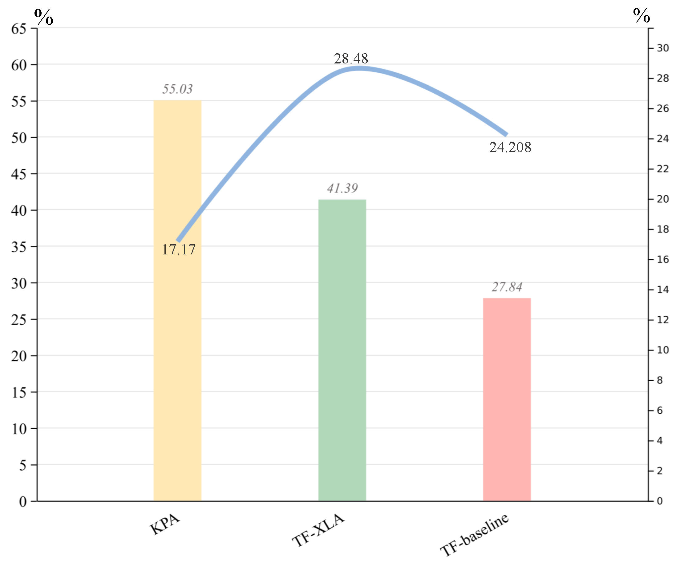
From the throughput evaluation (Figure 8), it can be observed that the proposed KPA method demonstrates more computing throughput, while XLA exhibits better performance in terms of memory throughput. The KPA approach reconstructs the computation graph of the Koopman operator and applies fine-grained parallel strategies during internal computations, which includes loop unrolling within kernel functions and instruction-level parallelism, leading to the enhanced computational performance observed in KPA. On the other hand, XLA achieves higher memory throughput owing to its ability to perform real-time computation graph analysis, reuse intermediate memory results, and automatically optimize the computational pipeline within the framework. This memory-aware optimization gives XLA an advantage in memory access efficiency. As further illustrated by the stacked bar in Figure 9, KPA shows suboptimal performance in data loading and memory access compared to XLA.
In our experiments, we used the maximum absolute error (MAE) to assess the difference between our study and TF-baseline and TF-XLA. It is mainly a measure of the maximum difference between the predicted values of each sample. The MAE is defined as follows:
M A E m a x = max i | y ˜ i ( b a s e l i n e ) y i ( K P A ) |
M A E m a x = max i | y ˜ i ( X L A ) y i ( K P A ) |

4.3.2. Ablation Study

To systematically assess the impact of key parameters on the parallel optimization of the Koopman operator, we conduct ablation experiments in this section. The experiments focus on evaluating the effects of shared and global memory chunk sizes, as well as the number of CUDA Streams, on computational performance. In this study, the shared memory chunks adopt block sizes consistent with those used for global memory (i.e., BLOCK_SIZE × BLOCK_SIZE). This consistent design ensures proper size alignment and enables coalesced access to global memory. Considering that the feature dimension of the CAFUC dataset is 265, which is not divisible by 8/16/32, we design the memory chunks accordingly to ensure efficient memory access. Specifically, thread blocks are sized as BLOCK_SIZE, and shared memory is allocated as [BLOCK_SIZE][BLOCK_SIZE + 1] to avoid bank conflicts during access. We do not further increase the chunk size, as the datasets used in the current experiments consist of short time-series, with limited data volume at each time step. Excessively large chunk sizes would result in under-utilization of threads within each thread block, thereby reducing parallel efficiency.
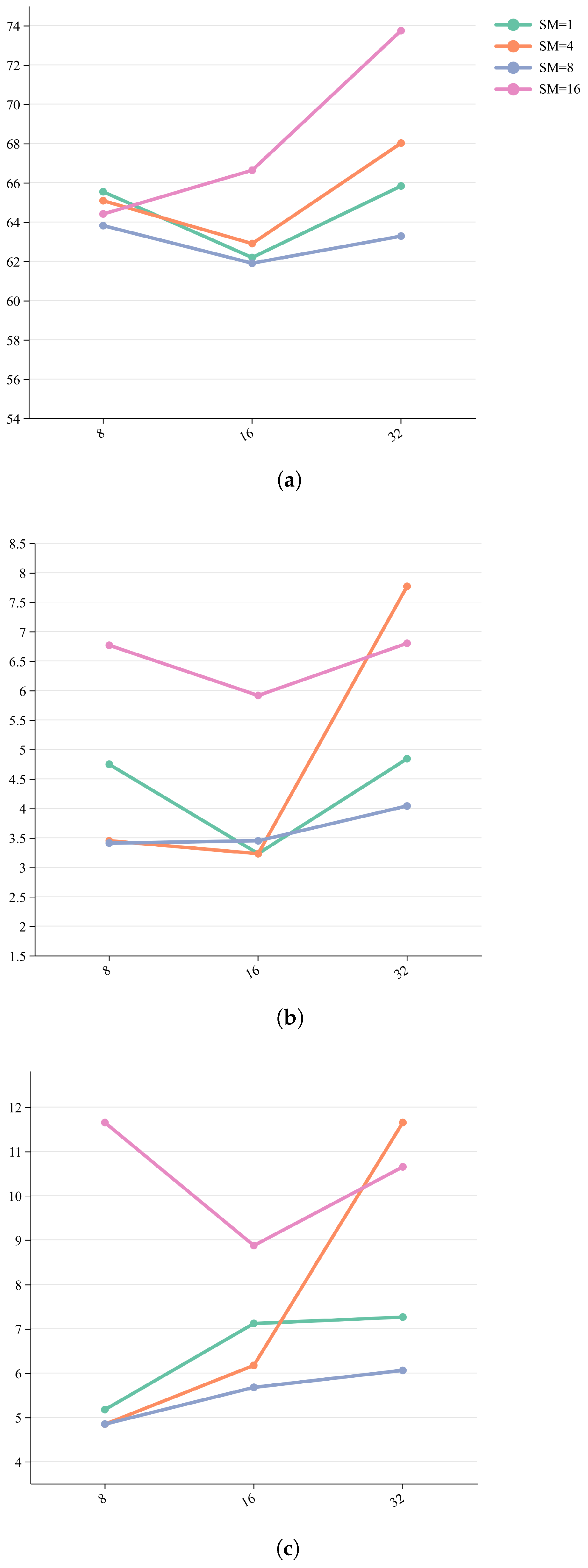
This experiment breaks down the computational process of the Koopman operator and records the time consumption at each stage. The results shown in Figure 10 indicate that when SM = 1, the time consumption of the two key computational stages is relatively high. This suggests that a single CUDA Stream does not effectively achieve parallel task distribution, and resource contention during the process leads to increased synchronization wait times. When SM = 8, lower time consumption is observed across all stages. However, when the number of streams is increased to 16, evident resource waste occurs, and the acceleration effect is not significantly improved.
When the shared memory block size (BLOCK_SIZE) is adjusted from 8 to 16, the time consumption in both the data loading and matrix computation stages decreases (Figure 10a,b), mainly due to the optimization of data locality in shared memories. Nevertheless, the pseudo-inverse solving process experiences an increase in computational complexity due to the larger block size, resulting in higher time consumption for SVD computation. Additionally, when BLOCK_SIZE is less than 32, increasing the number of SMs significantly reduces the time consumption, but when the shared memory block size reaches 32, further increases in the number of SMs do not show significant performance gains. The results suggest that, in this study, the optimal acceleration is achieved when BLOCK_SIZE = 16 and SM = 8. It should also be noted from Figure 10c that the computational aspect of the SVD is still a clear bottleneck for scalability, and future research efforts will focus on improvements in this area.

5. Conclusions

In this study, we proposed KPA, a CUDA-based parallel optimization algorithm, to address the computational bottlenecks in Koopman operator approximation and improve execution efficiency without compromising model accuracy. An experimental scenario using the Koopman operator solving the flight trajectory prediction is implemented, and its performance advantage is verified through benchmarking and ablation experiments. Experiments show that in the multidimensional flight trajectory prediction model, compared with the XLA framework acceleration and the tensorflow native framework acceleration, KPA can achieve higher computational throughput in the Koopman operator computation, and the advantage of KPA is more obvious with the increase in feature dimensions and dataset size.
When designing the KPA, for the sake of Koopman’s computational scalability, a modular operator solver interface was designed for the SVD part, with the ability to choose between a full pseudo-inverse or a truncated SVD depending on the actual application, which enables the KPA to be reused in other modeling tasks. According to the ablation study, we found that SVD computations remain a dominate bottleneck.
Nevertheless, several limitations remain. Pseudo-inverse computation still represents a major bottleneck despite kernel-level parallelization, hankering for hybrid or randomized SVD methods. Additionally, the static block-size strategy may not achieve optimal performance for highly variable feature dimensions, suggesting adaptive partitioning strategies for future work. Finally, the integration of KPA into differentiable pipelines and its interaction with automatic graph optimizers like XLA are promising directions for future research.
Based on the results of this study, the following directions can be explored:
(1)
Optimizing pseudo-inverse computation. As shown in Figure 9, pseudo-inverse calculation remains the dominant cost in the KPA pipeline, even after kernel-level optimizations. Future work could explore randomized SVD, low-rank approximations, or hybrid GPU-CPU solvers to further reduce this bottleneck.
(2)
Adaptive kernel and memory tuning. Current block-size configuration is static, optimized for a specific feature dimension and GPU architecture. A promising direction is to design auto-tuning frameworks that dynamically adjust thread/block configurations and memory partitioning based on runtime profiling and problem size.
(3)
Currently, the KPA is an external operator. Later studies can consider integrating KPAs into differentiable pipelines and interacting with automatic graph optimizers such as XLA to further improve overall performance and scalability.

Author Contributions

Conceptualization, methodology, data curation, J.L.; software, validation, writing—original draft, L.W.; investigation, writing—review and editing, supervision, Z.S. All authors have read and agreed to the published version of the manuscript.

Funding

This work is supported by the General Aviation Safety Operation Digital Intelligence Research Institute (TD2025DZ06) and the Fundamental Research Funds for the Central Universities (Scientific Project of Civil Aviation Flight University of China) under grant number 25CAFUC08001, 25CAFUC08002, and 24CAFUC03040.

Data Availability Statement

The original contributions presented in the study are included in the article, further inquiries can be directed to the corresponding author.

Conflicts of Interest

The authors declare no conflicts of interest. The funders had no role in the design of the study, in the collection, analyses, or interpretation of the data, in the writing of the manuscript, or in the decision to publish the results.

References

  1. Koopman, B.O. Hamiltonian systems and transformation in Hilbert space. Proc. Natl. Acad. Sci. USA 1931, 17, 315–318. [Google Scholar] [CrossRef] [PubMed]
  2. Bevanda, P.; Sosnowski, S.; Hirche, S. Koopman operator dynamical models: Learning, analysis and control. Annu. Rev. Control 2021, 52, 197–212. [Google Scholar] [CrossRef]
  3. Brunton, S.L.; Budišić, M.; Kaiser, E.; Kutz, J.N. Modern Koopman theory for dynamical systems. arXiv 2021, arXiv:2102.12086. [Google Scholar] [CrossRef]
  4. Kutz, J.N.; Brunton, S.L.; Brunton, B.W.; Proctor, J.L. Dynamic Mode Decomposition: Data-Driven Modeling of Complex Systems; SIAM: Philadelphia, PA, USA, 2016. [Google Scholar]
  5. Schmid, P.J. Dynamic mode decomposition of numerical and experimental data. J. Fluid Mech. 2010, 656, 5–28. [Google Scholar] [CrossRef]
  6. Haseli, M.; Cortés, J. Parallel learning of Koopman eigenfunctions and invariant subspaces for accurate long-term prediction. IEEE Trans. Control Netw. Syst. 2021, 8, 1833–1845. [Google Scholar] [CrossRef]
  7. Lusch, B.; Kutz, J.N.; Brunton, S.L. Deep learning for universal linear embeddings of nonlinear dynamics. Nat. Commun. 2018, 9, 4950. [Google Scholar] [CrossRef]
  8. Otto, S.E.; Rowley, C.W. Linearly recurrent autoencoder networks for learning dynamics. SIAM J. Appl. Dyn. Syst. 2019, 18, 558–593. [Google Scholar] [CrossRef]
  9. Brissette, C.; Hawkins, W.; M. Slota, G. GNN Node Classification Using Koopman Operator Theory on GPU. In Proceedings of the International Conference on Complex Networks and Their Applications, Istanbul, Türkiye, 10–12 December 2024; Springer: Cham, Switzerland, 2024; pp. 62–73. [Google Scholar]
  10. NVIDIA Corporation. cuSOLVER Library Documentation. 2025. Available online: https://docs.nvidia.com/cuda/cusolver/index.html (accessed on 31 August 2025).
  11. NVIDIA Corporation. Accelerating Linear Algebra with cuBLAS. 2025. Available online: https://docs.nvidia.com/cuda/cublas/index.html (accessed on 31 August 2025).
  12. Lu, J.; Jiang, J.; Bai, Y.; Dai, W.; Zhang, W. FlightKoopman: Deep Koopman for Multi-Dimensional Flight Trajectory Prediction. Int. J. Comput. Intell. Appl. 2025, 24, 2450038. [Google Scholar] [CrossRef]
  13. Pouria Talebi, S.; Kanna, S.; Xia, Y.; Mandic, D.P. A distributed quaternion Kalman filter with applications to fly-by-wire systems. In Proceedings of the 2016 IEEE International Conference on Digital Signal Processing (DSP), Beijing, China, 16–18 October 2016; pp. 30–34. [Google Scholar] [CrossRef]
  14. Liu, C.; Wang, J.; Zhang, W.; Yang, X.D.; Guo, X.; Liu, T.; Su, X. Synchronization of broadband energy harvesting and vibration mitigation via 1:2 internal resonance. Int. J. Mech. Sci. 2025, 301, 110503. [Google Scholar] [CrossRef]
  15. Shi, H.; Meng, M.Q.H. Deep Koopman operator with control for nonlinear systems. IEEE Robot. Autom. Lett. 2022, 7, 7700–7707. [Google Scholar] [CrossRef]
  16. Xiong, W.; Huang, X.; Zhang, Z.; Deng, R.; Sun, P.; Tian, Y. Koopman neural operator as a mesh-free solver of non-linear partial differential equations. J. Comput. Phys. 2024, 513, 113194. [Google Scholar] [CrossRef]
  17. Yeung, E.; Kundu, S.; Hodas, N. Learning deep neural network representations for Koopman operators of nonlinear dynamical systems. In Proceedings of the 2019 American Control Conference (ACC), Philadelphia, PA, USA, 10–12 July 2019; pp. 4832–4839. [Google Scholar]
  18. Boehm, M.; Reinwald, B.; Hutchison, D.; Evfimievski, A.V.; Sen, P. On optimizing operator fusion plans for large-scale machine learning in systemml. arXiv 2018, arXiv:1801.00829. [Google Scholar] [CrossRef]
  19. Chen, Y.; Brock, B.; Porumbescu, S.; Buluç, A.; Yelick, K.; Owens, J.D. Atos: A task-parallel GPU dynamic scheduling framework for dynamic irregular computations. arXiv 2021, arXiv:2112.00132. [Google Scholar] [CrossRef]
  20. Ekelund, J.; Markidis, S.; Peng, I. Boosting Performance of Iterative Applications on GPUs: Kernel Batching with CUDA Graphs. arXiv 2025, arXiv:2501.09398. [Google Scholar]
  21. Veneva, M.; Imamura, T. ML-Based Optimum Number of CUDA Streams for the GPU Implementation of the Tridiagonal Partition Method. arXiv 2025, arXiv:2501.05938. [Google Scholar] [CrossRef]
  22. Balagafshe, R.G.; Akoushideh, A.; Shahbahrami, A. Matrix-matrix multiplication on graphics processing unit platform using tiling technique. Indones. J. Electr. Eng. Comput. Sci. 2022, 28, 1012–1019. [Google Scholar] [CrossRef]
  23. Volkov, V.; Demmel, J.W. Benchmarking GPUs to tune dense linear algebra. In Proceedings of the SC’08: Proceedings of the 2008 ACM/IEEE Conference on Supercomputing, Austin, TX, USA, 15–21 November 2008; pp. 1–11. [Google Scholar]
  24. Adámek, K.; Dimoudi, S.; Giles, M.; Armour, W. GPU fast convolution via the overlap-and-save method in shared memory. ACM Trans. Archit. Code Optim. (TACO) 2020, 17, 18. [Google Scholar] [CrossRef]
  25. Abdelfattah, A.; Keyes, D.; Ltaief, H. Kblas: An optimized library for dense matrix-vector multiplication on gpu accelerators. ACM Trans. Math. Softw. (TOMS) 2016, 42, 18. [Google Scholar] [CrossRef]
  26. Sitchinava, N.; Weichert, V. Bank Conflict Free Comparison-based Sorting On GPUs. arXiv 2013, arXiv:1306.5076. [Google Scholar]
  27. Daga, T.; Bhanpato, J.; Behere, A.; Mavris, D. Aircraft Takeoff Weight Estimation for Real-World Flight Trajectory Data Using CNN-LSTM. In Proceedings of the AIAA Aviation Forum and ASCEND 2024, Las Vegas, NV, USA, 29 July–2 August 2024; p. 4291. [Google Scholar]
  28. Lu, J.; Chai, H.; Jia, R. A general framework for flight maneuvers automatic recognition. Mathematics 2022, 10, 1196. [Google Scholar] [CrossRef]
  29. Lai, G.; Chang, W.C.; Yang, Y.; Liu, H. Modeling long- and short-term temporal patterns with deep neural networks. In Proceedings of the The 41st International ACM SIGIR Conference on Research & Development in Information Retrieval, Ann Arbor, MI, USA, 8–12 July 2018; pp. 95–104. [Google Scholar]
  30. Wu, H.; Xu, J.; Wang, J.; Long, M. Autoformer: Decomposition transformers with auto-correlation for long-term series forecasting. Adv. Neural Inf. Process. Syst. 2021, 34, 22419–22430. [Google Scholar]
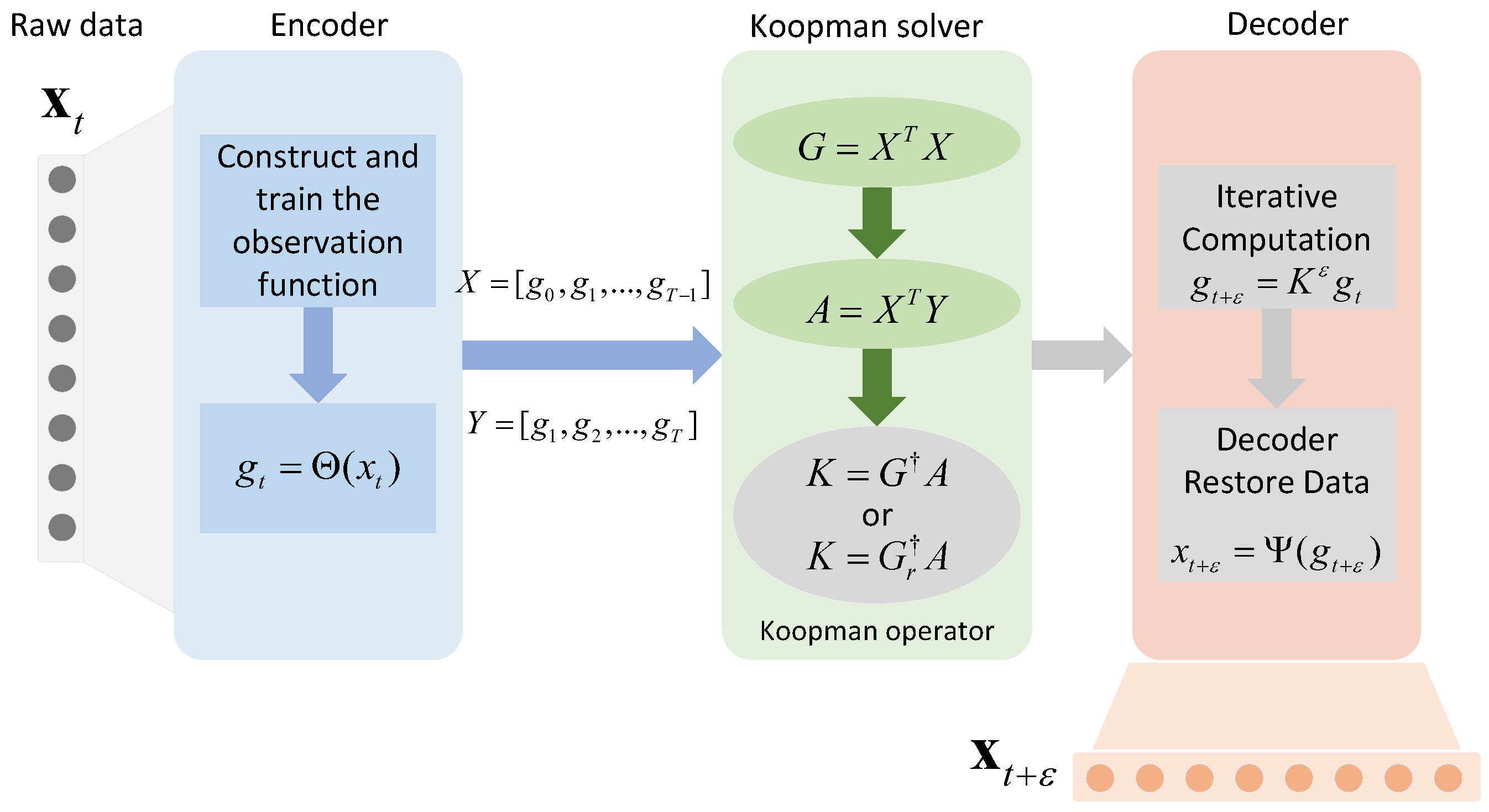
Figure 1. The complete framework for solving the Koopman operator using neural network training in a data-driven approach consists of three main components: the encoder, which extracts features from the original data to construct the observation function; the Koopman solver, which uses the data matrix generated by the encoder to perform a linear transformation that approximates the Koopman operator; and the decoder, which maps the state g t in the Koopman observation space back to the original trajectory space to obtain the future state data. The overall structure is illustrated in Figure 1. The individual components of this framework are described in the following sections.
Electronics 14 03609 g001
Figure 2. Analysis of dependencies among operators.
Electronics 14 03609 g002
Figure 3. The computational flow of Algorithm 1. Functions performed by the three kernel functions are designated.
Electronics 14 03609 g003
Figure 4. The dimension reorganization strategy. The blue cuboid on the left is three-dimensional data, which originally need to be co-indexed by the B and T dimensions. After dimensional reorganization, the input data become X R ( B × T ) × N . The computation requires consecutive pairs of states, so we get a total of B × ( T 1 ) sets.
Electronics 14 03609 g004
Figure 5. The process of double-buffer loading data, simultaneously completing data loading and data calculation. The left is the timeline, and right buffer 0 and buffer 1 are two buffers.
Electronics 14 03609 g005
Figure 6. Trajectories for the four training maneuver routes of Tear-Drop, Rectangle, Steep-turn, and Eight-turn. They are visualized using normalization to the same origin and projected to a 2D coordinate system.
Electronics 14 03609 g006
Figure 7. (a) Comparison of time consumption for single Koopman computation across six datasets under three frameworks. (b) Acceleration ratios for the three frameworks. Execution time of a single Koopman computation for three experimental configurations, with TF-Baseline as the reference. The acceleration ratio is calculated by first computing the ratio for each of the three methods on each dataset and then taking the average across all six datasets. To provide a more intuitive comparison of the advantages of our algorithm, the absolute execution time is also reported. Since the time consumed by each dataset does not vary by an order of magnitude or more, the absolute time shown in the figure represents the average across all datasets for each method. It can be observed that TF-Baseline primarily relies on frame scheduling and management, resulting in high computational time (251.17 ms on average). Enabling XLA compilation and optimization in TF-XLA significantly reduces execution time through static graph fusion and memory pre-allocation, achieving a speed up ratio of 2.26×. The KPA proposed in this study further reduces the execution time via an explicit CUDA parallelization strategy, with a speed up ratio of 2.47×; however, the improvement over TF-XLA is moderate (1.09×).
Electronics 14 03609 g007
Figure 8. Dual Y-axis plot showing the computing throughput (left Y-axis) and memory throughput (right Y-axis) for three frames. KPA performs better in terms of compute throughput, but its memory throughput is not as efficient as the other two’s that benefit from framework-based automatic optimization.
Electronics 14 03609 g008
Figure 9. Stacked bar chart of KPA showing the time distribution across different stages of a single iteration. Memory copying and data transfer constitute the largest portion of execution time.
Electronics 14 03609 g009
Figure 10. These three charts present the time distribution across different computational stages under various shared memory partitioning and numbers of streaming multiprocessors (SMs). (a) The data loading phase is the least time-consuming with BLOCKSIZE = 16 and SM = 8. (b) The matrix computation phase of the operator computation is the least time consuming with BLOCKSIZE = 16, SM = 4 and 1. However, the overall time consumed for SM = 8 is the lowest. (c) The pseudo-inverse computation phase of the operator computation is the least time-consuming with BLOCKSIZE = 16 and SM = 8.
Electronics 14 03609 g010
Table 1. Core operators in the network layer of the Koopman neural operator.
NameTypeInput DependenciesOutput Usage
Slice x i
Slice y i
Sliceinputs_arraytemp_A and temp_G
at each sampling index
matmul( x i T , x i )
matmul( x i T , y i )
MatMul x i , y i temp_G, temp_A
Accumulate G
Accumulate A
Addtemp_G and G
temp_A and A
G and A for
the next iteration
G = ( 1 / n _ G ) × G
A = ( 1 / n _ A ) × A
ScalarMulThe accumulation
of G and A
Input for K = G A
matmul(pinv(G), A)MatMulG, A K = G A
matmul(inputs, k)MatMulinputs, kModel Output
Table 2. Evaluation metrics and definitions.
Metric CategoryMetric NameDefinition
Time PerformanceIteration TimeThe time required to complete one Koopman operator computation.
Speed up RatioThe ratio of execution times between different implementation methods.
Resource EfficiencyComputational ThroughputThe ratio of kernel computational performance to the theoretical peak performance of the GPU.
Memory ThroughputThe efficiency of memory access during kernel execution.
Accuracy EvaluationAbsolute ErrorThe degree of difference between the optimized method and the original method.
Table 3. Notions and descriptions.
NotionDescription
TF-baselineNative Koopman Operator Based on TensorFlow
TF-XLATF-Baseline with XLA for Faster and More Efficient Execution
KPACustomized Koopman Operator Based on CUDA C++
Disclaimer/Publisher’s Note: The statements, opinions and data contained in all publications are solely those of the individual author(s) and contributor(s) and not of MDPI and/or the editor(s). MDPI and/or the editor(s) disclaim responsibility for any injury to people or property resulting from any ideas, methods, instructions or products referred to in the content.