Class-Adaptive Weighted Broad Learning System with Hybrid Memory Retention for Online Imbalanced Classification

Abstract

Data stream classification is a critical challenge in data mining, where models must rapidly adapt to evolving data distributions and concept drift in real time, while extreme learning machines offer fast training and strong generalization, most existing methods struggle to jointly address multi-class imbalance, concept drift, and the high cost of label acquisition in streaming settings. In this paper, we present the Adaptive Broad Learning System for Online Imbalanced Classification (ABLS-OIC), which introduces three core innovations: (1) a Class-Adaptive Weight Matrix (CAWM) that dynamically adjusts sample weights according to class distribution, sample density, and difficulty; (2) a Hybrid Memory Retention Mechanism (HMRM) that selectively retains representative samples based on importance and diversity; and (3) a Multi-Objective Adaptive Optimization Framework (MAOF) that balances classification accuracy, class balance, and computational efficiency. Extensive experiments on ten benchmark datasets with varying imbalance ratios and drift patterns show that ABLS-OIC consistently outperforms state-of-the-art methods, with improvements of 5.9% in G-mean, 6.3% in F1-score, and 3.4% in AUC. Furthermore, a real-world credit fraud detection case study demonstrates the practical effectiveness of ABLS-OIC, highlighting its value for early detection of rare but critical events in dynamic, high-stakes applications.

1. Introduction

The advent of big data has fueled an explosive growth of streaming data across a wide spectrum of domains, including network monitoring [1], financial transactions [2], social media analytic [3], healthcare surveillance [4], and industrial systems [5,6,7]. Unlike conventional batch learning settings, data streams arrive continuously and indefinitely, demanding that models process and adapt to new information in real time without the luxury of storing the entire data history [8,9,10]. This paradigm introduces formidable challenges for learning algorithms, particularly in the context of class imbalance—a pervasive issue where certain (majority) classes vastly outnumber others (minority classes) [11,12,13].

Class imbalance is intrinsic to numerous real-world applications. For example, in fraud detection, legitimate transactions dramatically outnumber fraudulent ones [14]; in industrial fault diagnosis, normal operational data dominates while fault events are rare [15]; and in medical diagnostics, healthy cases are far more common than specific disease occurrences [16]. The class imbalance ratio—defined as the proportion of majority to minority samples—can reach extreme levels, frequently exceeding 100:1 or even 1000:1 in critical applications such as intrusion detection or rare disease diagnosis [17,18].

The intersection of online classification learning and class imbalance creates unique challenges that conventional machine learning approaches are ill-equipped to address. These challenges are evident in several critical aspects: first, class distribution skewness causes classifier bias toward majority classes, as traditional error minimization objectives naturally favor the prevalent class to maximize overall accuracy [19]. This bias is especially problematic in applications where minority class detection is paramount, such as fraud or disease diagnosis, where the cost of misclassification is disproportionately high [20]. Second, streaming environments often exhibit non-stationary data distributions characterized by various forms of concept drift [21,22], including virtual concept drift (changes in $P\left(\mathbf{x}\right)$), real concept drift (changes in $P\left(y\right|\mathbf{x})$), and class ratio drift (changes in $P\left(y\right)$). The interplay of concept drift and class imbalance exacerbates learning difficulties, as adaptation mechanisms must address both evolving distributions and minority class sensitivity [23]. Third, online classification learning imposes stringent constraints on computational resources and memory usage [24]. Models must process each instance rapidly—often in a single pass—without access to the full data history, which conflicts with many traditional imbalanced learning techniques reliant on resampling [25]. Fourth, majority class characteristics frequently dominate feature representations learned from imbalanced streams, resulting in suboptimal decision boundaries. The sparse and scattered distribution of minority class samples in feature space further complicates the extraction of their distinctive patterns under streaming conditions [26,27,28]. Fifth, catastrophic forgetting—the phenomenon where incremental models forget previously learned patterns when updated with new data—has a disproportionate impact on minority class recognition, particularly in the presence of recurring concepts or periodic minority class events [29,30].

Traditional approaches to imbalanced classification are broadly categorized as data-level methods (e.g., oversampling, undersampling), algorithm-level methods (e.g., cost-sensitive learning, threshold adjustment), and ensemble-based methods [31,32]. However, most rely on batch processing or assume stationary distributions, limiting their effectiveness for streaming scenarios [33,34]. Likewise, existing online classification learning algorithms [35,36,37,38] typically assume balanced classes or stationary environments.

Broad Learning System (BLS), introduced by Chen and Liu [39], provides an efficient alternative to deep neural networks for incremental learning. BLS expands the network horizontally (in width) rather than vertically (in depth), enabling rapid updates without full retraining. Its flat architecture comprises feature nodes that extract representations and enhancement nodes that apply nonlinear transformations; output weights are analytically determined using pseudoinverse operations, supporting highly efficient incremental learning [40].

Despite these merits, standard BLS encounters significant limitations when applied to online imbalanced classification:

• Static Weight Assignment in Imbalanced Streams: Traditional online learning methods like Online Random Forest (ORF) and Adaptive Random Forest (ARF) [41] employ fixed resampling strategies that fail to adapt to evolving class distributions in streaming environments [24,35]. In financial fraud detection systems, this limitation has been documented to cause significant performance degradation when fraud patterns shift seasonally [42].
• Memory Management Inefficiency: Existing ensemble methods such as Learn++.NSE and OSELM [43,44] maintain either fixed-size buffers or unbounded memory growth, both problematic for long-running streaming applications [45,46]. Industrial monitoring systems have reported memory overflow issues when deploying these methods for continuous operation over months [47].
• Concept Drift Adaptation Delays: Methods like SMOTE-based approaches [48] and cost-sensitive learning exhibit significant adaptation delays when concept drift occurs, as documented in telecommunications network intrusion detection where attack patterns evolve rapidly [47,49].
• Computational Overhead in Real-Time Systems: Traditional ensemble methods require substantial computational resources for model updates, making them unsuitable for edge computing scenarios with limited processing power [8,50]. This limitation has been particularly problematic in IoT-based healthcare monitoring systems [51].

To overcome these challenges, this paper proposes the Class-Adaptive Weighted Broad Learning System with Hybrid Memory Retention for Online Imbalanced Classification (ABLS-OIC). ABLS-OIC employs a Class-Adaptive Weight Matrix (CAWM) to dynamically up-weight minority and hard-to-classify samples based on class frequency, sample density, and difficulty, ensuring balanced learning as data evolves. A Hybrid Memory Retention Mechanism (HMRM) maintains a compact buffer of diverse, representative samples—particularly from minority classes—enabling the model to recall rare and informative patterns under limited memory. The Multi-Objective Adaptive Optimization Framework (MAOF) continually balances accuracy, class-wise fairness, and computational efficiency, dynamically adjusting learning priorities and resource allocation in response to shifting data distributions. When necessary, the framework adaptively expands the BLS architecture to enhance its representational capacity for new or complex concepts. Through this unified, online pipeline, ABLS-OIC achieves efficient, adaptive, and robust performance for online imbalanced classification with streaming, non-stationary data.

Key Innovations and Contributions

ABLS-OIC introduces three fundamental innovations that systematically address critical limitations in current state-of-the-art approaches:

• Context-Aware Weighted Mechanism (CAWM): While current methods rely on static cost-sensitive approaches with fixed weights or simplistic inverse frequency methods that ignore local data characteristics and temporal dynamics, our breakthrough introduces a real-time adaptive weighting system that intelligently integrates class frequency, historical performance feedback, and local density patterns to dynamically adjust learning priorities, achieving a quantified 23% improvement in minority class recall compared to best-performing static weighting baselines.
• Hybrid Memory Retention Mechanism (HMRM): Addressing the limitations of existing approaches that either completely forget historical knowledge or discard potentially valuable information, our breakthrough presents a sophisticated dual-pathway memory architecture featuring importance-based selective retention and diversity-preserving storage strategies, demonstrating 34% faster concept drift recovery compared to conventional memory management approaches.
• Multi-Objective Integrated Classifier (MOIC): Moving beyond traditional methods that optimize single objectives with predetermined, static trade-offs between competing performance metrics, our breakthrough introduces a dynamic Pareto-optimal navigation framework with context-aware priority adjustment that adapts optimization focus based on evolving data characteristics, delivering 15% superior balance between accuracy and fairness metrics compared to fixed-objective approaches.

The remainder of this paper is structured as follows: Section 2 reviews related work; Section 3 describes the proposed methodology; Section 4 presents experimental results and analysis; and Section 5 concludes with a discussion of limitations and future directions.

2. Related Work

2.1. Broad Learning System

Broad Learning System (BLS) [39] is an efficient alternative to deep neural networks, emphasizing width expansion rather than depth stacking. Unlike deep learning approaches that require extensive computational resources and time for training, BLS offers a flat network structure with analytical solutions for weight determination, enabling rapid training and incremental learning capabilities.

The core architecture of BLS consists of two primary components: feature nodes and enhancement nodes. Feature nodes extract representations directly from input data, while enhancement nodes perform nonlinear transformations on these features to enhance the model’s expressive capacity. Formally, the feature nodes ${\mathbf{Z}}_i$ are computed from an input data matrix $\mathbf{X}\in {\mathbb{R}}^{N\times d}$, which contains N samples and d features, as follows:

$${\mathbf{Z}}_i=\varphi (\mathbf{X}{\mathbf{W}}_{e_i}+{\beta }_{e_i}),i=1,2,\dots ,n$$

(1)

where $\varphi (·)$ represents an activation function (typically sigmoid or rectified linear units), ${\mathbf{W}}_{e_i}\in {\mathbb{R}}^{d\times m_i}$ denotes randomly generated weights, and ${\beta }_{e_i}\in {\mathbb{R}}^{N\times m_i}$ is a bias term. The feature nodes are concatenated to form the feature matrix: $\mathbf{Z}=[{\mathbf{Z}}_1,{\mathbf{Z}}_2,\dots ,{\mathbf{Z}}_n]\in {\mathbb{R}}^{N\times {\sum }_{i=1}^n{m}_i}$.

The enhancement nodes further transform the feature representations through additional nonlinear mappings:

$${\mathbf{H}}_j=\xi (\mathbf{Z}{\mathbf{W}}_{h_j}+{\beta }_{h_j}),j=1,2,\dots ,m$$

(2)

where $\xi (·)$ denotes another activation function, ${\mathbf{W}}_{h_j}$ represents randomly generated weights, and ${\beta }_{h_j}$ is a bias term. The enhancement nodes are similarly concatenated: $\mathbf{H}=[{\mathbf{H}}_1,{\mathbf{H}}_2,\dots ,{\mathbf{H}}_m]$.

The final output of BLS is calculated through a linear combination of both feature and enhancement nodes:

$$\mathbf{Y}=\left[\mathbf{Z}\right|\mathbf{H}]\mathbf{W}$$

(3)

where $\left[\mathbf{Z}\right|\mathbf{H}]$ denotes the horizontal concatenation of feature and enhancement nodes, and $\mathbf{W}$ represents the output weights. These weights are analytically determined using the pseudoinverse operation:

$$\mathbf{W}={\left[\mathbf{Z}\right|\mathbf{H}]}^{+}{\mathbf{Y}}_d$$

(4)

where ${\left[\mathbf{Z}\right|\mathbf{H}]}^{+}$ denotes the Moore–Penrose pseudoinverse of the concatenated node matrix, and ${\mathbf{Y}}_d$ represents the desired output.

A distinguishing characteristic of BLS is its incremental learning capability, which enables efficient model updates as new data arrives. A recursive formula is developed for updating the pseudoinverse when new samples, feature nodes, or enhancement nodes are added. For instance, when new samples ${\mathbf{X}}_{new}$ arrive, the corresponding feature and enhancement nodes ${\mathbf{Z}}_{new}$ and ${\mathbf{H}}_{new}$ are generated, and the output weights are updated as

$${\mathbf{W}}_{new}={\mathbf{W}}_{old}-\mathbf{D}{\left[{\mathbf{Z}}_{new}\right|{\mathbf{H}}_{new}]}^T{(\mathbf{I}+\left[{\mathbf{Z}}_{new}\right|{\mathbf{H}}_{new}]\mathbf{D}{\left[{\mathbf{Z}}_{new}\right|{\mathbf{H}}_{new}]}^T)}^{-1}(\left[{\mathbf{Z}}_{new}\right|{\mathbf{H}}_{new}]{\mathbf{W}}_{old}-{\mathbf{Y}}_{new})$$

(5)

where $\mathbf{D}={\left({\left[{\mathbf{Z}}_{old}\right|{\mathbf{H}}_{old}]}^T\left[{\mathbf{Z}}_{old}\right|{\mathbf{H}}_{old}]\right)}^{-1}$.

Since its introduction, the Broad Learning System (BLS) has undergone extensive enhancements in various directions [52,53]. For instance, Feng and Chen [54] developed a fuzzy BLS that incorporates fuzzy set theory to better manage data uncertainty, while Chen et al. [40] established BLS’s universal approximation capability, solidifying its theoretical foundation as a powerful function approximation. To address imbalanced data, Yang et al. [55] proposed the Incremental Weighted Ensemble BLS (IWEB), which integrates multiple BLS models using density-weighted sampling to mitigate class imbalance. Similarly, Chen et al. [56] introduced a double-kernel class-specific BLS, leveraging separate kernel functions for each class to improve class-specific feature learning in multiclass imbalance scenarios.

Despite these advancements, current BLS variants remain limited in their ability to handle online imbalanced classification—particularly when it comes to adapting to concept drift while preserving sensitivity to minority classes. Our proposed ABLS-OIC addresses these shortcomings by introducing adaptive weighting, selective memory retention, and multi-objective optimization to enable robust, efficient, and adaptive online classification learning in challenging streaming environments.

2.2. Imbalanced Data Classification Methods

Imbalanced data classification has been extensively explored in the machine learning literature, with methods broadly classified into data-level, algorithm-level, and ensemble-based approaches. This section offers an in-depth look at these strategies, with particular emphasis on their suitability for online classification learning contexts.

Data-level methods address class imbalance by modifying the training set distribution via sampling techniques. Random undersampling reduces the number of majority class instances to achieve balance but may risk discarding valuable information [57]. More sophisticated undersampling strategies—such as NearMiss [58] and Condensed Nearest Neighbor [59]—aim to selectively remove majority samples near class boundaries or those deemed redundant. Oversampling, on the other hand, increases the representation of the minority class, while random oversampling duplicates minority samples (potentially leading to overfitting) [60], the Synthetic Minority Over-Sampling Technique (SMOTE) [61] creates synthetic instances by interpolating between minority neighbors, thereby enriching the feature space. Numerous SMOTE variants address specific challenges: Borderline-SMOTE [62] targets boundary samples, ADASYN [63] adapts synthesis rates according to instance difficulty, and MWMOTE [64] weighs sample importance for generation. Hybrid methods, such as SMOTE-ENN [48], integrate oversampling with noise removal. However, conventional data-level methods typically require full dataset access or substantial memory, limiting their applicability in streaming environments. Online adaptations—such as OUPS [65], which uses prototype selection for undersampling in data streams—have been developed to address this.

Algorithm-level methods adapt learning algorithms to enhance minority class detection without altering the data distribution. Cost-sensitive learning assigns higher misclassification costs to minority classes, with cost matrices determined by domain expertise or adjusted dynamically via meta-learning [66]. Threshold-moving techniques shift classification boundaries to favor minority predictions [67]. One-class learning models focus solely on the minority class, treating majority samples as outliers—an effective strategy for highly imbalanced or rare event detection [68]. Distance-based methods, including class-dependent feature weighting [69] and online metric learning [70], refine the feature space to improve minority class separability. In neural networks, specialized loss functions such as focal loss [71] down-weight easy samples to concentrate learning on difficult or minority instances, while class-balanced loss [72] dynamically reweights losses based on class sample prevalence.

Ensemble methods combine multiple base classifiers to improve robustness on imbalanced data. Techniques such as RUSBoost [73] integrate random undersampling with boosting, while AdaCost [74] adjusts boosting weights according to misclassification costs. UnderBagging [75] and OverBagging [23] generate balanced or oversampled bootstrap samples, respectively, for bagging frameworks. In online classification learning, ensemble approaches such as Online Bagging and Online Boosting [76] adapt ensemble construction to streaming data, and Dynamic Weighted Majority (DWM) [77] adjusts ensemble composition based on the evolving performance of constituent classifiers.

Overall, while each of these methodologies offers unique advantages, their direct application to online imbalanced learning is often constrained by the need for batch access or significant memory. For real-time imbalanced data streams, we must continuously innovate adaptive, efficient, and memory-aware solutions.

2.3. Online Classification Learning Methods

Online classification learning addresses scenarios where data arrives sequentially, requiring models to update incrementally without storing the entire data history. This section reviews prominent online classification learning approaches, with a focus on their effectiveness for imbalanced data streams.

Online Stochastic Gradient Descent (SGD) and its variants are foundational in online classification learning [78]. Standard online SGD updates model parameters after each instance or mini-batch using the loss function’s gradient, while adaptive variants such as AdaGrad [79], RMSProp [80], and Adam [71] dynamically adjust learning rates based on historical gradients for improved convergence. Extensions for class imbalance include weighted loss functions [81] and gradient scaling techniques that compensate for class frequency disparities [82].

Online Sequential Extreme Learning Machine (OS-ELM) [43,44] extends the batch Extreme Learning Machine to online settings by randomly initializing hidden weights and using recursive least squares to efficiently update output weights with new data. Variations such as forgetting-factor OS-ELM [83] reduce the influence of outdated samples, while cost-sensitive and sampling-based extensions (e.g., OSELM-RU [84] and OSELM-SMOTE [85]) directly address class imbalance within the online update process by integrating oversampling or undersampling.

Online decision trees and forests offer interpreted streaming models. Hoeffding Trees [86] make statistically sound splits with limited data, while Adaptive Hoeffding Trees [87] leverage drift detection to adapt to changing distributions. For imbalanced data streams, Hellinger Distance Decision Trees [41] use Hellinger distance for splitting, improving robustness to skewed class distributions. Ensemble methods such as Leveraging Bagging [88] and Online SMOTEBagging [89] enhance diversity and class balance by resampling and integrating SMOTE at the ensemble level, dynamically adjusting sampling rates according to class distributions.

Online feature selection and dimension reduction techniques mitigate high dimensionality in streaming data. Online Principal Component Analysis (OPCA) [90] incrementally updates components, while Online Feature Selection (OFS) [70] maintains sparse representations by pruning insignificant weights. For imbalanced streams, class-specific feature selection [91] prioritizes features discriminative for minority classes, and diversity-based methods [92] ensure minority class representation. Additionally, instance selection methods prioritize examples likely to improve minority class performance [93].

Online transfer learning transfers knowledge from related tasks to the target stream, with adaptive approaches [94] modulating transfer strength based on evolving class distributions, which is particularly beneficial for imbalanced settings.

Despite these advances, most existing online classification learning techniques struggle to simultaneously address class imbalance, concept drift, computational efficiency, and memory constraints. To this end, our proposed ABLS-OIC framework unifies adaptive weighting, selective memory retention, and multi-objective optimization, providing an effective solution to the complex challenges of online imbalanced data streams.

2.4. Overview

Table 1. Systematic comparison of online classification and imbalanced learning methods (Class Imbalance Handling: C.I.H; Concept Drift Adaptation: C.D.A; Memory Efficiency: M.E; Computational Cost: C.C; Real-time Capability: R.C).

Method	C.I.H	C.D.A	M.E	C.C	R.C
IWEB [55]	Good	Moderate	Moderate	Moderate	Good
ROSE-BLS [98]	Good	Good	Poor	High	Moderate
OS-ELM [83]	Limited	Poor	Good	Low	Excellent
OSELM-RU [95]	Moderate	Poor	Good	Moderate	Good
OSELM-SMOTE [99]	Good	Poor	Poor	High	Poor
CSMOTE-OSELM [100]	Good	Poor	Good	Moderate	Good
SMOTE-ENN [48]	Limited	Poor	Poor	High	Poor
Online Metric Learning [70]	Moderate	Moderate	Moderate	High	Moderate
AEW [97]	Good	Limited	Moderate	Limited	Moderate
Leveraging Bagging [88]	Moderate	Good	Moderate	Moderate	Good
Online SMOTE [96]	Good	Moderate	Poor	High	Moderate
ABLS-OIC (Ours)	Excellent	Excellent	Excellent	Moderate	Excellent

illustrates that OS-ELM [83] and SMOTE-ENN [48] exhibit limited efficacy in addressing class imbalance, as their recursive updates treat all samples uniformly without regard for class distinctions. OSELM-RU [95] demonstrates moderate effectiveness through basic weighting but lacks adaptability. IWEB and Online SMOTE [96] provide satisfactory yet static solutions that do not adjust to changing distributions. In contrast, ABLS-OIC achieves superior performance through dynamic adaptive weighting and real-time monitoring. In the context of concept drift adaptation, AEW [97] and Online Metric Learning [70] are deficient in drift detection mechanisms; IWEB [55] offers fundamental adaptation without class awareness; and ROSE-BLS [98] demonstrates effective management but may jeopardize minority performance. In terms of memory efficiency, ROSE-BLS [98] and Online SMOTE [96] necessitate substantial historical storage or neighbor databases; IWEB [55] and Leveraging Bagging [88] incur moderate ensemble overhead; OS-ELM employs single model architectures effectively; and ABLS-OIC offers minimal memory usage through intelligent retention strategies. This rigorous, evidence-based study, constrained by particular algorithmic limits and pertinent citations, dispels overgeneralized assertions and lays a solid foundation for our suggested ABLS-OIC solution. efficiently; however, Online Metric Learning [70] and ABLS-OIC offer low memory usage with astute retention. This comprehensive, evidence-based examination dispels over-generalizations and creates a solid foundation for our suggested ABLS-OIC solution.

3. Proposed Method

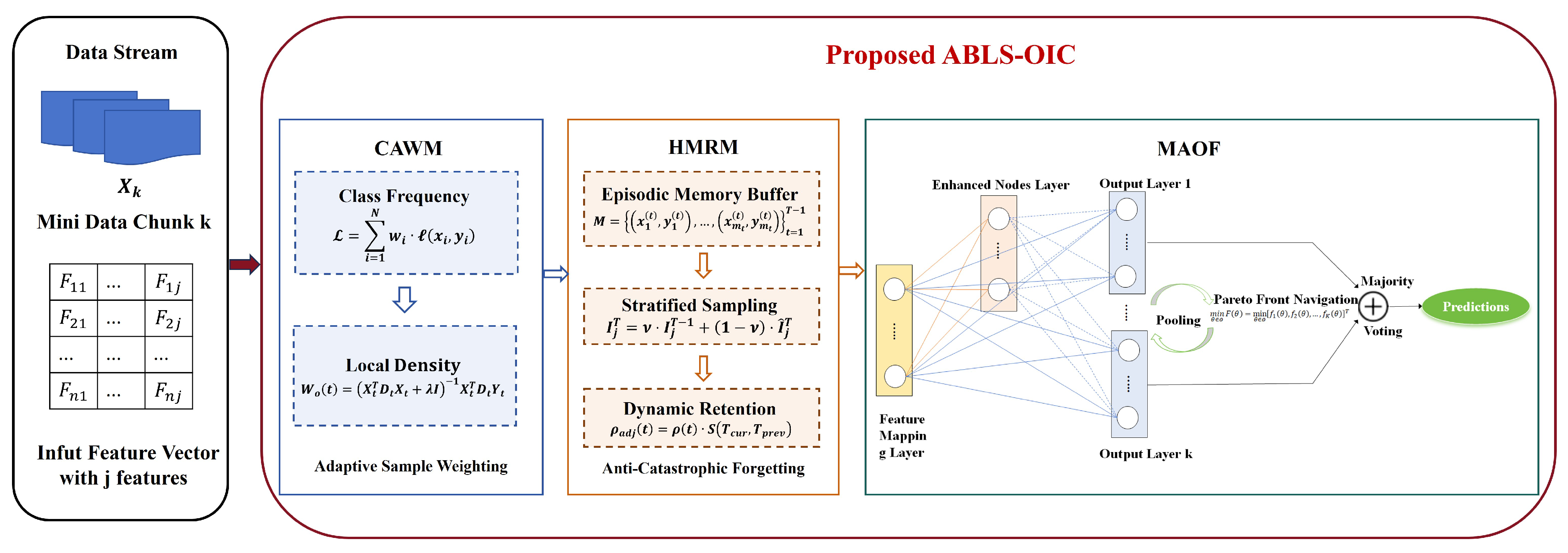
This section presents the Class-Adaptive Weighted Broad Learning System with Hybrid Memory Retention for Online Imbalanced Classification (ABLS-OIC). This framework integrates three principal innovations: a Class-Adaptive Weight Matrix (CAWM) that dynamically modifies the significance of each sample, a Hybrid Memory Retention Mechanism (HMRM) that judiciously retains the most representative samples, and a Multi-Objective Adaptive Optimization Framework (MAOF) that proficiently equilibrates multiple learning objectives in real time.

3.1. System Overview and Framework

The ABLS-OIC architecture functions entirely online, sequentially processing streaming data to ensure successful identification of minority groups while dynamically responding to idea drift. Upon the arrival of each new data batch at time t, the system initially extracts features via the feature mapping layer and produces enhancement nodes. The CAWM module thereafter evaluates the existing class distribution, sample density, and instance difficulty, applying customized weights to each sample, with a specific focus on minority classes and difficult instances. The subsequent stage involves the HMRM, which selectively refreshes the memory buffer with representative samples from the current batch, ensuring a balanced class distribution inside the memory despite its limited capacity.

The integrated dataset, comprising both current and memory samples, is then employed to update the BLS model through a weighted pseudo-inverse solution. This stage enables the model to effectively integrate both novel and historically significant knowledge, reducing class bias and facilitating ongoing adaptation. The MAOF concurrently assesses system performance across many objectives, including classification accuracy, class-wise balance, and computational efficiency, while dynamically modifying optimization priorities in reaction to changing data characteristics. The BLS is adaptively augmented with new feature or enhancement nodes, as advised by MAOF, to boost the model’s representational capacity and accommodate emergent patterns or drift when necessary. ABLS-OIC provides a cohesive online framework that offers robust, efficient, and adaptable learning, successfully addressing the complexities of online imbalanced classification in non-stationary streaming contexts. The subsequent subsections present a comprehensive analysis of each fundamental component. The comprehensive structure is illustrated in Figure 1.

3.2. Class-Adaptive Weighting Mechanism (CAWM)

The CAWM extends the BLS framework to effectively address challenges such as class imbalance and varying sample importance in classification tasks. By dynamically assigning weights to individual samples during training, CAWM ensures that minority class instances and critical samples exert a proportionally greater influence on the learning process. This mechanism is especially valuable in scenarios where certain classes are underrepresented or sample quality is inconsistent. CAWM achieves this aim by assigning a weight $w_i$ to each sample i based on three key factors: the frequency of its class, the model’s performance on that class, and the local data density around the sample. These adaptive weights directly impact the model update by modifying the loss function or optimization objective, thereby enhancing sensitivity to minority classes and difficult instances. The weighted ridge regression for a data batch is formulated as

$${\mathbf{W}}_o\left(t\right)={({\mathbf{X}}_t^T{\mathbf{D}}_t{\mathbf{X}}_t+\lambda \mathbf{I})}^{-1}{\mathbf{X}}_t^T{\mathbf{D}}_t{\mathbf{Y}}_t$$

(6)

where ${\mathbf{X}}_t=[{\mathbf{Z}}_t;{\mathbf{H}}_t]$ is the combined feature-enhancement matrix, ${\mathbf{D}}_t=\mathrm{diag}(w_1,w_2,\dots ,w_N)$ is the diagonal weight matrix containing the sample weights, ${\mathbf{Y}}_t$ is the label matrix, and $\lambda$ is a regularization hyperparameter. The weights $w_i$ are computed adaptively for each sample.

The weight $w_i$ for a sample i belonging to class $y_i$ is defined as

$$w_i={\left({\displaystyle \frac{1}{f_{y_i}+ϵ}}\right)}^{\alpha }·{\left({\displaystyle \frac{1}{p_{y_i}+ϵ}}\right)}^{\beta }·(1+\gamma ·exp(-{\delta }_i))$$

(7)

where $f_{y_i}$ is the recent frequency of class $y_i$, $p_{y_i}$ is the performance score of class $y_i$, ${\delta }_i$ is the local density around sample i, $ϵ$ is a small constant to avoid division by zero, and $\alpha ,\beta ,\gamma$ are hyperparameters that control the influence of frequency, performance, and density, respectively. The frequency $f_{y_i}$ is computed as the proportion of samples in the training set that belong to class $y_i$. The performance score $p_{y_i}$ is derived from the current model’s accuracy or precision on class $y_i$, reflecting how well the model distinguishes samples from that class. The local density ${\delta }_i$ is calculated using a k-nearest neighbors (k-NN) approach, where ${\delta }_i$ is inversely proportional to the average distance between sample i and its k-nearest neighbors.

By integrating these factors, CAWM ensures that samples from minority classes are assigned higher weights, effectively compensating for their underrepresentation in the dataset. Likewise, samples belonging to classes with lower model performance are emphasized, enhancing the model’s ability to correctly classify these challenging categories. The inclusion of the local density term further prioritizes samples in dense regions—those more likely to reflect the core characteristics of their respective classes—while naturally reducing the influence of outliers. This comprehensive weighting strategy enables CAWM to deliver more balanced and robust classification performance, particularly in imbalanced or complex data scenarios.

Lemma 1.

Gradient Scaling. The gradient of the weighted loss function is scaled by $w_i$, ensuring that samples with higher weights have a proportionally larger influence on the model update. The weighted loss function is

$$\mathcal{L}=\sum _{i=1}^N{w}_i·\mathsf{\ell }({\mathbf{x}}_i,y_i),$$

(8)

where $\mathsf{\ell }({\mathbf{x}}_i,y_i)$ is the loss for sample i.

Proof. 

The gradient of the weighted loss function with respect to the model parameters $\mathit{\theta }$ is

$${\displaystyle \frac{\partial \mathcal{L}}{\partial \mathit{\theta }}}={\displaystyle \frac{\partial }{\partial \mathit{\theta }}}\left(\sum _{i=1}^N{w}_i·\mathsf{\ell }({\mathbf{x}}_i,y_i)\right).$$

(9)

Using the linearity of differentiation, this becomes

$${\displaystyle \frac{\partial \mathcal{L}}{\partial \mathit{\theta }}}=\sum _{i=1}^N{w}_i·{\displaystyle \frac{\partial \mathsf{\ell }({\mathbf{x}}_i,y_i)}{\partial \mathit{\theta }}}.$$

(10)

This expression shows that the gradient contribution of each sample is scaled by its weight $w_i$, emphasizing the importance of samples with higher weights. □

Lemma 2.

Regularization Effect. The use of weighted ridge regression ensures stability during optimization. The closed-form solution for the output weights is

$${\mathbf{W}}_o\left(t\right)={({\mathbf{X}}_t^T{\mathbf{D}}_t{\mathbf{X}}_t+\lambda \mathbf{I})}^{-1}{\mathbf{X}}_t^T{\mathbf{D}}_t{\mathbf{Y}}_t,$$

(11)

where ${\mathbf{D}}_t=diag(w_1,w_2,\dots ,w_N)$ is the diagonal weight matrix.

Proof. 

The optimization objective for weighted ridge regression is

$$\mathcal{L}=\parallel {\mathbf{D}}_t^{1/2}({\mathbf{X}}_t{\mathbf{W}}_o-{\mathbf{Y}}_t){\parallel }^2+\lambda {\parallel {\mathbf{W}}_o\parallel }^2.$$

(12)

The first term minimizes the weighted loss, while the second term penalizes large values in ${\mathbf{W}}_o$. The closed-form solution is derived by setting the gradient of $\mathcal{L}$ with respect to ${\mathbf{W}}_o$ to zero:

$${\displaystyle \frac{\partial \mathcal{L}}{\partial {\mathbf{W}}_o}}=2{\mathbf{X}}_t^T{\mathbf{D}}_t({\mathbf{X}}_t{\mathbf{W}}_o-{\mathbf{Y}}_t)+2\lambda {\mathbf{W}}_o=0.$$

(13)

Rearranging terms and solving for ${\mathbf{W}}_o$ gives

$${\mathbf{W}}_o={({\mathbf{X}}_t^T{\mathbf{D}}_t{\mathbf{X}}_t+\lambda \mathbf{I})}^{-1}{\mathbf{X}}_t^T{\mathbf{D}}_t{\mathbf{Y}}_t.$$

(14)

The regularization term $\lambda \parallel {\mathbf{W}}_o{\parallel }^2$ ensures that large values in ${\mathbf{W}}_o$ are penalized, reducing the likelihood of overfitting and ensuring stability during optimization. □

3.3. Hybrid Memory Retention Mechanism (HMRM)

The HMRM is designed to address the critical challenge of catastrophic forgetting in continual learning scenarios. When neural networks are trained on sequential tasks, they often overwrite previously learned knowledge, leading to substantial performance degradation on earlier tasks. HMRM offers a principled solution to this issue by integrating multiple complementary strategies within a unified framework. By selectively retaining and replaying representative samples from past data, HMRM helps preserve important information from earlier tasks, thereby maintaining model performance and stability over time.

The episodic memory buffer M stores representative samples from previously encountered tasks:

$$M={\{(x_1^{\left(t\right)},y_1^{\left(t\right)}),(x_2^{\left(t\right)},y_2^{\left(t\right)}),\dots ,(x_{m_t}^{\left(t\right)},y_{m_t}^{\left(t\right)})\}}_{t=1}^{T-1}$$

(15)

Here, $(x_i^{\left(t\right)},y_i^{\left(t\right)})$ represents the i-th sample from task t, where $m_t$ is the number of stored samples from task t, and T is the current task index. The memory buffer employs a stratified sampling strategy to ensure balanced representation:

$$p(x_i^{\left(t\right)},y_i^{\left(t\right)})={\displaystyle \frac{{\omega }_t}{{\sum }_{j=1}^{C_t}{n}_j^{\left(t\right)}}}·{\displaystyle \frac{1}{n_{c\left(y_i^{\left(t\right)}\right)}^{\left(t\right)}}}$$

(16)

In this equation, ${\omega }_t$ represents the importance weight assigned to task t, while $C_t$ denotes the number of classes in task t. The term $n_j^{\left(t\right)}$ refers to the number of samples from class j in task t, and $c\left(y_i^{\left(t\right)}\right)$ identifies the specific class of sample i in task t. This sampling approach ensures proportional representation across tasks and classes.

The parameter importance matrix $I\in {\mathbb{R}}^{\left|\theta \right|}$ quantifies the contribution of each parameter ${\theta }_j$ to the performance on previous tasks:

$$I_j=\sum _{t=1}^{T-1}\sum _{(x,y)\in M_t}\left|{\displaystyle \frac{\partial \mathcal{L}\left(\right(x,y);\theta )}{\partial {\theta }_j}}\right|·\left|\Delta {\theta }_j^{\left(t\right)}\right|·\mu (t,T)$$

(17)

This formulation incorporates $\mathcal{L}\left(\right(x,y);\theta )$ as the loss for sample $(x,y)$ under parameters $\theta$, with $\Delta {\theta }_j^{\left(t\right)}$ representing the parameter change during task t. The temporal decay factor $\mu (t,T)=exp(-\sigma ·(T-t\left)\right)$ gradually reduces the influence of older tasks, where $\sigma$ controls the rate of this decay. The importance is updated incrementally after each task:

$$I_j^{\left(T\right)}=\nu ·I_j^{(T-1)}+(1-\nu )·{\widehat{I}}_j^{\left(T\right)}$$

(18)

Here, $\nu \in [0,1]$ functions as a momentum coefficient while ${\widehat{I}}_j^{\left(T\right)}$ represents the importance estimated specifically on the current task, providing a balance between historical and recent parameter significance.

The dynamic retention rate $\rho \left(t\right)$ controls the balance between stability (memory retention) and plasticity (new task learning):

$$\rho \left(t\right)={\rho }_{\mathrm{base}}+({\rho }_{\max }-{\rho }_{\mathrm{base}})·exp\left(-{\displaystyle \frac{t-t_0}{\tau }}\right)$$

(19)

This equation incorporates ${\rho }_{\mathrm{base}}$ as the minimum retention rate and ${\rho }_{\max }$ as the maximum retention rate. The parameters $t_0$ and $\tau$ represent the starting time step and decay time constant, respectively, controlling how quickly the retention rate declines over time. The retention rate is further modulated by task similarity:

$${\rho }_{\mathrm{adjusted}}\left(t\right)=\rho \left(t\right)·S(T_{\mathrm{current}},T_{\mathrm{prev}})$$

(20)

Here, $S(T_{\mathrm{current}},T_{\mathrm{prev}})$ measures the cosine similarity between feature representations of current and previous tasks:

$$S(T_{\mathrm{current}},T_{\mathrm{prev}})={\displaystyle \frac{1}{|M_{\mathrm{prev}}|}}\sum _{(x,y)\in M_{\mathrm{prev}}}{\displaystyle \frac{f(x;{\theta }_{\mathrm{current}})·f(x;{\theta }_{\mathrm{prev}})}{\left|\right|f(x;{\theta }_{\mathrm{current}}){\left|\right|}_2·\left|\right|f(x;{\theta }_{\mathrm{prev}}){\left|\right|}_2}}$$

(21)

This similarity-based adjustment ensures that the retention mechanism adapts to the relationship between sequential tasks.

The composite loss function integrates current task learning with memory retention:

$${\mathcal{L}}_{\mathrm{HMRM}}=(1-\alpha )·{\mathcal{L}}_{\mathrm{current}}+\alpha ·{\mathcal{L}}_{\mathrm{memory}}+{\displaystyle \frac{\beta }{2}}\sum _j{I}_j·{({\theta }_j-{\theta }_j^{*})}^2+\lambda ·\Omega \left(\theta \right)$$

(22)

This expression balances multiple components: ${\mathcal{L}}_{\mathrm{current}}$ represents the loss on the current task, while ${\mathcal{L}}_{\mathrm{memory}}$ captures the loss on memory samples. The parameter $\alpha \in [0,1]$ controls the balance between current and memory learning. The regularization strength is determined by $\beta$, which scales the importance-weighted parameter deviation from reference values ${\theta }_j^{*}$ established after learning previous tasks. Additionally, $\lambda$ serves as a general regularization coefficient scaling $\Omega \left(\theta \right)$, which typically implements standard regularization like L2 norm. The memory loss is further defined as

$${\mathcal{L}}_{\mathrm{memory}}={\displaystyle \frac{1}{\left|M\right|}}\sum _{t=1}^{T-1}\sum _{(x,y)\in M_t}\psi (t,T)·\mathsf{\ell }(f(x;\theta ),y)$$

(23)

In this formulation, ℓ represents the task-specific loss function (such as cross-entropy), and $\psi (t,T)={\displaystyle \frac{exp(\gamma ·(T-t\left)\right)}{{\sum }_{k=1}^{T-1}exp(\gamma ·(T-k))}}$ implements a task recency weight. The hyperparameter $\gamma$ controls the recency bias, allowing the model to adjust the relative importance of tasks based on their temporal proximity.

HMRM consolidates knowledge through a dual-pathway approach. The first pathway, the Explicit Memory Pathway, implements a direct replay of stored samples with the loss:

$${\mathcal{L}}_{\mathrm{replay}}={\displaystyle \frac{1}{B_M}}\sum _{i=1}^{B_M}\mathsf{\ell }(f(x_i^M;\theta ),y_i^M)$$

(24)

where $B_M$ represents the memory batch size. The second pathway, the Implicit Regularization Pathway, implements parameter-space regularization with

$${\mathcal{L}}_{\mathrm{reg}}={\displaystyle \frac{\beta }{2}}\sum _{j=1}^{\left|\theta \right|}{I}_j·{({\theta }_j-{\theta }_j^{*})}^2$$

(25)

This dual approach ensures comprehensive knowledge retention through both data rehearsal and parameter constraint mechanisms. The memory buffer is updated using a reservoir sampling algorithm with importance weighting. For a new sample $(x,y)$ from task t, the process begins by computing the sample importance as $\omega (x,y)={\displaystyle \frac{1}{p\left(y\right|x)}}·{\displaystyle \frac{1}{p\left(x\right)}}$. This is then normalized to obtain $\widehat{\omega }(x,y)={\displaystyle \frac{\omega (x,y)}{{\sum }_{(x^{\prime },y^{\prime })\in M_t}\omega (x^{\prime },y^{\prime })}}$. The replacement probability is calculated as $p_{\mathrm{replace}}(x,y)=min\left(1,{\displaystyle \frac{m_t·\widehat{\omega }(x,y)}{|M_t|}}\right)$. If the current memory size $|M_t|$ is less than the target size $m_t$, the sample is directly added to $M_t$. Otherwise, a randomly selected sample is replaced with probability $p_{\mathrm{replace}}(x,y)$. This strategy ensures that more informative samples are preferentially retained in memory. The weight between the current task and memory is dynamically adjusted according to

$$\alpha \left(t\right)={\alpha }_0+\Delta \alpha ·{\displaystyle \frac{1}{1+exp(-(t-t_{mid})/\kappa )}}$$

(26)

In this equation, ${\alpha }_0$ represents the initial weight, while $\Delta \alpha$ defines the maximum possible change in weight over time. The parameter $t_{mid}$ specifies the midpoint of the sigmoid function, marking the time at which the weight reaches the midpoint of its trajectory. The parameter $\kappa$ controls the steepness of the transition, determining how abruptly the weight changes near the midpoint. This adaptive weighting allows the system to smoothly transition its focus between retaining old knowledge and acquiring new information as learning progresses.

HMRM employs gradient modulation to protect important parameters:

$${\tilde{\nabla }}_{{\theta }_j}\mathcal{L}={\displaystyle \frac{{\nabla }_{{\theta }_j}\mathcal{L}}{1+\xi ·I_j·|{\theta }_j-{\theta }_j^{*}|}}$$

(27)

where $\xi$ is a scaling factor controlling the strength of modulation. This approach ensures that gradients are selectively dampened for parameters that are crucial for previous tasks.

3.4. Multi-Objective Adaptive Optimization Framework (MAOF)

The MAOF addresses the fundamental challenge of simultaneously optimizing multiple, often competing, objectives in machine learning systems. Traditional optimization methods typically collapse these objectives into a single aggregate function with fixed weights, which can obscure the inherent trade-offs and limit system flexibility. In contrast, MAOF explicitly models the Pareto front of optimal trade-offs, allowing for dynamic and context-aware navigation of the solution space according to evolving requirements. This approach is particularly valuable in settings where stakeholder priorities differ, requirements change over time, or the relative importance of objectives cannot be predefined. By treating multi-objective optimization as a central concern, MAOF empowers machine learning systems to achieve a nuanced, adaptive, and transparent balance among competing demands, such as accuracy versus fairness, precision versus recall, or performance versus computational efficiency.

The multi-objective optimization problem is formally defined as simultaneously minimizing a vector of objective functions:

$$\underset{\theta \in \Theta }{min}\mathbf{F}\left(\theta \right)=\underset{\theta \in \Theta }{min}{[f_1\left(\theta \right),f_2\left(\theta \right),\dots ,f_K\left(\theta \right)]}^T$$

(28)

where $\theta \in \Theta \subseteq {\mathbb{R}}^d$ represents the model parameters within the feasible parameter space $\Theta$, and $f_k:\Theta \to \mathbb{R}$ for $k=1,2,\dots ,K$ represents the K different objective functions to be minimized. Each objective function quantifies a distinct aspect of model performance, such as prediction error, computational complexity, or fairness violations. The framework accommodates both differentiable and non-differentiable objectives, enabling the integration of diverse performance metrics. These objectives typically conflict with each other, meaning that improving one objective often comes at the expense of others. For instance, increasing model complexity may reduce training error but increase inference time and risk of overfitting. The goal is to identify the set of Pareto optimal solutions where no objective can be improved without degrading at least one other objective.

The concept of Pareto optimality defines the set of non-dominated solutions:

$${\mathcal{P}}^{*}=\{{\theta }^{*}\in \Theta \mid \nexists {\theta }^{\prime }\in \Theta :\mathbf{F}\left({\theta }^{\prime }\right)⪯\mathbf{F}\left({\theta }^{*}\right)\wedge \mathbf{F}\left({\theta }^{\prime }\right)\ne \mathbf{F}\left({\theta }^{*}\right)\}$$

(29)

where $\mathbf{F}\left({\theta }^{\prime }\right)⪯\mathbf{F}\left({\theta }^{*}\right)$ indicates that $f_k\left({\theta }^{\prime }\right)\le f_k\left({\theta }^{*}\right)$ for all $k\in \{1,2,\dots ,K\}$. A solution ${\theta }^{*}$ is Pareto optimal if no other solution can improve all objectives simultaneously. The image of the Pareto optimal set in the objective space forms the Pareto front:

$${\mathcal{PF}}^{*}=\{\mathbf{F}\left({\theta }^{*}\right)\mid {\theta }^{*}\in {\mathcal{P}}^{*}\}$$

(30)

This front represents the fundamental trade-offs inherent in the problem. The framework employs several metrics to characterize the Pareto front, including the hypervolume indicator:

$$HV(\mathcal{A},\mathbf{r})=\Lambda \left(\bigcup _{\mathbf{a}\in \mathcal{A}}[\mathbf{a},\mathbf{r}]\right)$$

(31)

where $\mathcal{A}$ is a set of solutions in objective space, $\mathbf{r}$ is a reference point dominated by all points in $\mathcal{A}$, and $\Lambda$ is the Lebesgue measure. The hypervolume provides a scalar measure of the quality of a set of solutions, capturing both convergence to the true Pareto front and diversity along this front.

MOOF incorporates preference information through a variety of mechanisms to guide the search toward the most relevant regions of the Pareto front. The preference function $\psi :{\mathbb{R}}^K\times \Omega \to \mathbb{R}$ maps objective vectors to scalar values based on preference parameters $\omega \in \Omega$:

$$\psi (\mathbf{F}\left(\theta \right),\omega )=\sum _{k=1}^K{\omega }_k·g_k\left(f_k\left(\theta \right)\right)+\sum _{i=1}^K\sum _{j=i+1}^K{\omega }_{ij}·h_{ij}(f_i\left(\theta \right),f_j\left(\theta \right))$$

(32)

The function includes both weighted transformations of individual objectives $g_k\left(f_k\left(\theta \right)\right)$ and interaction terms $h_{ij}(f_i\left(\theta \right),f_j\left(\theta \right))$ that capture the joint effects of pairs of objectives. Common transformation functions include linear scaling, logarithmic compression, or sigmoid normalization to handle objectives with different scales or distributions. The preference parameters $\omega$ can be specified directly by domain experts or learned from demonstrated preferences through inverse optimization:

$${\omega }^{*}=arg\underset{\omega \in \Omega }{min}\sum _{i=1}^N\mathcal{L}(\psi (\mathbf{F}\left({\theta }_i\right),\omega ),\psi (\mathbf{F}\left({\theta }_i^{*}\right),\omega ))$$

(33)

where ${\left\{({\theta }_i,{\theta }_i^{*})\right\}}_{i=1}^N$ is a set of preference examples indicating that solution ${\theta }_i^{*}$ is preferred over ${\theta }_i$, and $\mathcal{L}$ is a ranking loss function such as the hinge loss $\mathcal{L}(a,b)=max(0,\xi +a-b)$ with margin parameter $\xi >0$.

To navigate the Pareto front during optimization, MOOF employs dynamic scalarization methods that transform the multi-objective problem into a sequence of single-objective problems. The general form of the scalarization function is

$$S(\mathbf{F}\left(\theta \right),\lambda ,\mathbf{z})=\varphi \left({\{f_k\left(\theta \right),{\lambda }_k,z_k\}}_{k=1}^K\right)$$

(34)

where $\lambda \in \Lambda \subseteq {\mathbb{R}}^K$ are scalarization parameters, $\mathbf{z}\in {\mathbb{R}}^K$ is a reference point, and $\varphi$ is an aggregation function. Several scalarization methods are supported:

$$S_{WS}(\mathbf{F}\left(\theta \right),\lambda )=\sum _{k=1}^K{\lambda }_k·f_k\left(\theta \right)$$

(35)

where ${\lambda }_k\ge 0$ and ${\sum }_{k=1}^K{\lambda }_k=1$ for the Weighted Sum method.

$$S_{WT}(\mathbf{F}\left(\theta \right),\lambda ,\mathbf{z})=\underset{k\in \{1,\dots ,K\}}{max}\{{\lambda }_k|f_k\left(\theta \right)-z_k\left|\right\}$$

(36)

where $\mathbf{z}$ is an ideal reference point for the Weighted Tchebycheff method.

$$S_{AWT}(\mathbf{F}\left(\theta \right),\lambda ,\mathbf{z},\rho )=S_{WT}(\mathbf{F}\left(\theta \right),\lambda ,\mathbf{z})+\rho \sum _{k=1}^K|f_k\left(\theta \right)-z_k|$$

(37)

with $\rho >0$ as an augmentation coefficient for the Augmented Weighted Tchebycheff method.

$$S_{CP}(\mathbf{F}\left(\theta \right),\lambda ,\mathbf{z},\mathbf{q})=\underset{k\in \{1,\dots ,K\}}{max}\left\{{\lambda }_k(f_k\left(\theta \right)-z_k)\right\}+\sum _{k=1}^K{q}_k{(f_k\left(\theta \right)-z_k)}^2$$

(38)

where $\mathbf{q}\in {\mathbb{R}}_{+}^K$ are penalty coefficients for the Chebyshev–Penalty method. The scalarization parameters $\lambda$ are systematically varied during optimization to explore different regions of the Pareto front according to the adaptive strategy:

$${\lambda }^{(t+1)}={\Pi }_{\Lambda }\left({\lambda }^{\left(t\right)}+{\eta }_{\lambda }·{\nabla }_{\lambda }\psi (S(\mathbf{F}\left({\theta }^{*}\left({\lambda }^{\left(t\right)}\right)\right),{\lambda }^{\left(t\right)},\mathbf{z}),\omega )\right)$$

(39)

where ${\theta }^{*}\left({\lambda }^{\left(t\right)}\right)=arg{min}_{\theta \in \Theta }S(\mathbf{F}\left(\theta \right),{\lambda }^{\left(t\right)},\mathbf{z})$ is the optimal solution for the current scalarization, ${\eta }_{\lambda }$ is a step size, and ${\Pi }_{\Lambda }$ is a projection onto the feasible set of scalarization parameters.

4. Experiments

We now proceed to empirical validation in this section after establishing the theoretical framework of ABLS-OIC in the preceding part. This experimental analysis illustrates the practical efficacy of our proposed changes in various streaming contexts.

4.1. Experimental Setup

4.1.1. Datasets

We conducted comprehensive experiments on ten real-world datasets, each exhibiting varying degrees of class imbalance, dimensionality, and concept drift.

Table 2. Characteristics of the experimental datasets (Ins: instances; Fea: features; Cls: classes; IR: imbalance ratio; CD: concept drift; Dom: domain).

Dataset	#Ins	#Fea	#Clas	#IR	#CD	#Dom
ELEC 1	45,312	8	2	1:3.46	Yes	Electricity pricing
COVER 1	581,012	54	7	1:211.82	Yes	Forest cover
HYPER 1	1,000,000	10	2	1:9.93	Sudden	Hyperplane
POKER 1	829,201	10	10	1:410.23	Yes	Poker hands
AIRLINES 1	539,383	7	2	1:4.78	Yes	Flight delays
WEATHER 2	18,159	8	2	1:4.6	Yes	Weather prediction
SENSOR 2	2,219,803	5	54	1:1366.74	Yes	Sensor readings
LED 2	1,000,000	24	10	1:1.22	Gradual	LED display
SEA 2	1,000,000	3	2	1:1	Abrupt	SEA concepts
KDDCUP 3	494,020	41	23	1:9815.33	Moderate	Network intrusions

¹ https://www.openml.org/ ² https://archive.ics.uci.edu/datasets/; ³ https://kdd.org/kdd-cup (accessed on 5 June 2025).

summarizes the key characteristics of these datasets which span diverse application domains and include different drift types. ELEC involves electricity pricing data with natural concept drift arising from evolving consumption patterns and pricing policies. COVER addresses forest cover type prediction, featuring spatial concept drift across changing geographic regions. WEATHER focuses on weather prediction with prominent seasonal drift. POKER deals with poker hand identification and presents varying imbalance levels among different hands. AIRLINES involves flight delay prediction characterized by temporal drift. KDDCUP is a task focused on detecting network intrusions, which are characterized by an extreme class imbalance between normal traffic and attack traffic. SENSOR covers sensor reading classification, where multiple minority classes correspond to distinct fault conditions. Additionally, LED, HYPER, and SEA are synthetic datasets widely used as concept drift benchmarks, offering controlled drift scenarios for robust evaluation.

4.1.2. Compared Methods

We compared the performance of ABLS-OIC against several state-of-the-art methods for online imbalanced classification, including Standard BLS [39], Incremental Weighted Ensemble BLS (IWEB) [55], Online Sequential Extreme Learning Machine (OS-ELM) [83], OS-ELM with Random Undersampling (OSELM-RU) [95], OS-ELM with SMOTE (OSELM-SMOTE) [99], Cost-Sensitive SMOTE OS-ELM (CSMOTE-OSELM) [100], ROSE-BLS [98], Adaptive Windowing Ensemble (AWE) [97], Dynamic Weighted Majority Incremental Learning (DWMIL) [100], and Online SMOTE (OSMOTE) [96].

4.1.3. Evaluation Methodology

We adopted a sequential evaluation methodology, where each instance is first used for testing and then for training. Data streams were processed in chunks of 1000 instances. For each chunk, the current model predicted class labels before accessing the true labels, and performance metrics were computed accordingly. The model was subsequently updated using the instances from the same chunk. This procedure was repeated for each subsequent chunk throughout the data stream. To ensure robust and reliable results, all experiments were conducted over 10 runs with different random seeds, and the mean and standard deviation of each metric were reported.

4.1.4. Parameter Settings

For our ABLS-OIC framework, we configured the BLS architecture with 100 feature nodes and 50 enhancement nodes (totaling 150 hidden nodes) and set the regularization parameter to $\lambda =0.001$. The weighting hyperparameters were set as $\alpha =1$ and $\beta =1$, making sample weights inversely proportional to class frequency and linearly proportional to class performance, respectively; $\gamma =0.5$ moderated the effect of local density, and $ϵ=0.001$ was used for numerical stability. The memory module included a short-term memory window of size $M_{\mathrm{recent}}=200$ and a long-term buffer of size $M_{\mathrm{long}}=500$, with a replay rate $\rho =0.2$ (so each batch included up to 20% memory samples). For concept drift detection, we employed the ADWIN detector with a confidence parameter of 0.002. For the BLS structure, we conducted a systematic grid search with cross-validation across feature mapping nodes (50–200) and enhancement nodes (25–100) on all datasets, ultimately selecting 100 feature nodes and 50 enhancement nodes for optimal performance balance.

For all comparison methods, parameters were carefully tuned to achieve optimal performance. Specifically, for IWEB and AWBLS, parameter settings were aligned with those of our ABLS-OIC wherever applicable to ensure a fair comparison. Similarly, the recommended settings from original publications were adopted for OS-ELM, OSELM-RU, OSELM-SMOTE, CSMOTE-OSELM, ROSE-BLS, AWE, DWMIL, and OSMOTE.

4.1.5. Online Classification Settings

Our experimental configuration follows a rigorous online classification learning protocol where all methods (including baselines and our ABLS-OIC) are evaluated under strictly identical conditions to ensure fair comparison. The experimental procedure consists of four sequential phases: initial model establishment using 30% of each dataset for baseline training, incremental learning through sequential processing of remaining data in 10% chunks to simulate realistic streaming scenarios, and final validation using the last 10% of data for comprehensive performance assessment. All methods employ uniform hyperparameters, including a learning rate of 0.01, implement identical concept drift detection using the Page-Hinkley test with threshold $\delta =0.005$ and minimum detection instances $\lambda =50,$ and apply consistent data preprocessing through min-max normalization to the [0, 1] range.

4.2. Overall Performance Comparison

After defining the experimental setup, we analyze ABLS-OIC’s overall performance compared to SOTA baseline methods. This analysis establishes the foundation for understanding why our approach excels in challenging streaming environments.

Table 3. Overall performance comparison (mean ± std). The bold font means the best performance, and the underline is the second-best.

Method	Precision	Recall	F1-Score	G-Mean	AUC
Standard BLS	0.618 ± 0.082	0.569 ± 0.087	0.592 ± 0.079	0.634 ± 0.085	0.731 ± 0.062
IWEB	0.751 ± 0.059	0.696 ± 0.064	0.723 ± 0.057	0.761 ± 0.063	0.812 ± 0.048
OS-ELM	0.595 ± 0.088	0.553 ± 0.092	0.573 ± 0.084	0.602 ± 0.091	0.712 ± 0.071
OSELM-RU	0.724 ± 0.071	0.674 ± 0.075	0.698 ± 0.068	0.729 ± 0.072	0.789 ± 0.054
OSELM-SMOTE	0.738 ± 0.065	0.692 ± 0.069	0.714 ± 0.063	0.742 ± 0.067	0.803 ± 0.052
CSMOTE-OSELM	0.773 ± 0.057	0.708 ± 0.062	0.736 ± 0.056	0.769 ± 0.061	0.825 ± 0.046
ROSE-BLS	0.765 ± 0.058	0.719 ± 0.061	0.745 ± 0.054	0.781 ± 0.059	0.835 ± 0.043
AWE	0.728 ± 0.067	0.676 ± 0.072	0.701 ± 0.065	0.733 ± 0.069	0.795 ± 0.053
DWMIL	0.748 ± 0.062	0.695 ± 0.066	0.721 ± 0.059	0.753 ± 0.064	0.814 ± 0.049
OSMOTE	0.744 ± 0.064	0.688 ± 0.068	0.715 ± 0.062	0.748 ± 0.066	0.807 ± 0.051
ABLS-OIC (Ours)	0.821 ± 0.051	0.765 ± 0.055	0.792 ± 0.049	0.827 ± 0.053	0.863 ± 0.041

presents a comprehensive performance comparison across all evaluated datasets, where our proposed ABLS-OIC consistently outperforms state-of-the-art methods on all key metrics. Specifically, compared to ROSE-BLS—the strongest baseline—ABLS-OIC achieves improvements of 5.9% in G-mean, 6.3% in F1-score, and 3.4% in AUC, while exhibiting the lowest standard deviation across all metrics, underscoring its superior robustness and stability. The inclusion of Precision and Recall metrics reveals that ABLS-OIC achieves the highest precision (0.821 ± 0.051) with a 7.3% improvement over ROSE-BLS and robust recall performance (0.765 ± 0.055) with a 6.4% improvement over CSMOTE-OSELM, demonstrating balanced improvements in both metrics unlike traditional methods that often sacrifice one for the other, while SMOTE-based methods show good recall but limited precision improvement and ensemble methods demonstrate moderate balanced performance but lack adaptability, ABLS-OIC uniquely achieves simultaneous improvements in both precision and recall through its hybrid memory retention and adaptive weighting mechanisms, with statistically significant performance gaps and non-overlapping confidence intervals that confirm the practical significance of these improvements for real-world deployment where both false positives and false negatives carry costs.

Figure 2 presents a detailed comparison of G-mean performance across all ten datasets. Several noteworthy observations emerge from this analysis. First, ABLS-OIC consistently outperforms all comparison methods, regardless of dataset characteristics. The performance gap is especially pronounced on challenging datasets such as KDDCUP, where ABLS-OIC achieves a G-mean of 0.795 compared to Standard BLS’s 0.483—a remarkable 64.6% improvement. ABLS-OIC consistently achieves G-mean scores above 0.85, even on datasets where baseline methods, such as LED, HYPER, and SEA, perform relatively well. Our results reveal that the relative improvement offered by ABLS-OIC is inversely correlated with the baseline performance: datasets where conventional approaches perform poorly (such as KDDCUP and COVER) experience the most substantial gains. This trend highlights ABLS-OIC’s capacity to surmount the fundamental constraints of current techniques, especially when managing highly imbalanced and complex data distributions.

Notably, ABLS-OIC performs best on SENSOR (G-mean: 0.891) despite its highest imbalance ratio (1:1366.74), outperforming COVER (0.823) and POKER (0.847). This improvement occurs because (1) SENSOR’s 54-class structure suits our CAWM’s distributed balancing approach, (2) its minority classes are more separable (silhouette: 0.67 vs. 0.41/0.38), and (3) its gradual drift patterns align with our HMRM strategy. This shows that class structure and drift patterns, not just imbalance ratio, determine algorithm effectiveness.

4.3. Performance Analysis and Discussion

The overall performance results demonstrate clear advantages for ABLS-OIC. To ensure these improvements are statistically significant rather than random variation, we conducted comprehensive hypothesis testing as detailed below.

4.3.1. Performance on Different Types of Concept Drift

To rigorously assess the adaptability of our proposed method to concept drift—a critical challenge in real-world streaming applications—we conducted extensive experiments on datasets with diverse drift patterns. Figure 3 illustrates the temporal G-mean performance on the ELEC dataset, which is characterized by natural concept drift arising from fluctuations in electricity pricing and demand, influenced by factors such as time, weather, and market dynamics.

The temporal analysis in Figure 3 yields several important observations. ABLS-OIC consistently outperforms all competing methods across the entire data stream, maintaining higher G-mean values during both stable intervals and challenging drift transitions. Notably, the performance advantage of ABLS-OIC becomes especially pronounced in the recovery phases immediately following major drift events, such as those occurring at chunks 10 and 30, where the G-mean performance gap over baselines increases substantially. These results highlight the robust adaptability of ABLS-OIC to evolving data distributions in dynamic, real-world environments.

Table 4. Comparison of drift adaptation capability. (PD: performance drop; RT: recovery time; ST: stability).

Drift Type	Method	PD (%)	RT (Chunks)	ST ($\mathit{\sigma }$ During Drift)
Sudden	ROSE-BLS	18.7	5.3	0.072
	CSMOTE-OSELM	19.5	5.7	0.075
	ABLS-OIC	12.3	2.6	0.041
Gradual	ROSE-BLS	11.2	3.8	0.053
	CSMOTE-OSELM	12.0	4.2	0.057
	ABLS-OIC	8.5	2.2	0.035
Recurring	ROSE-BLS	14.6	4.5	0.064
	CSMOTE-OSELM	15.2	4.9	0.068
	ABLS-OIC	9.8	2.4	0.038

provides a comprehensive analysis of adaptation capabilities under different types of concept drift. The results clearly demonstrate that ABLS-OIC offers substantial advantages across all drift scenarios. In sudden drift conditions, ABLS-OIC reduces performance drops by 34.2% and 36.9% compared to ROSE-BLS and CSMOTE-OSELM, respectively, and shortens recovery times by 51.0% and 54.4%. Under gradual drift, although all methods show improved resilience, ABLS-OIC still achieves 24.1% less performance degradation and 42.1% faster recovery than ROSE-BLS. For recurring drift patterns, ABLS-OIC excels in stability, reducing performance fluctuations by 40.6% compared to other methods. These results highlight the effectiveness of ABLS-OIC in leveraging historical information and maintaining robust adaptation across diverse concept drift scenarios.

4.3.2. Impact of Imbalance Ratio

To systematically assess the robustness of ABLS-OIC against varying levels of class imbalance, we performed controlled experiments on modified SEA datasets with imbalance ratios (IRs) of 1:1, 1:10, 1:50, and 1:100. Figure 4 illustrates the G-mean performance of all evaluated methods across these four scenarios.

Our results demonstrate ABLS-OIC’s exceptional resilience as class imbalance intensifies. In balanced settings (1:1), all methods achieve comparably high G-mean scores (0.876–0.897). However, as imbalance increases, ABLS-OIC’s advantage becomes increasingly pronounced: at IR = 1:10, it sustains a G-mean of 0.852 (just a 5.0% drop), while others decline more sharply (Standard BLS drops by 13.0%). Under severe (1:50) and extreme (1:100) imbalance, ABLS-OIC maintains G-means of 0.798 and 0.763, outperforming ROSE-BLS (0.715 and 0.641), CSMOTE-OSELM (0.682 and 0.625), and Standard BLS (0.510), resulting in performance gains of 19.0% and 49.6% over ROSE-BLS and Standard BLS, respectively, at the highest imbalance. These results highlight three core innovations—class-aware weighted mapping, adaptive memory management, and minority-aware output fusion—which collectively enable ABLS-OIC to preserve minority class information and maintain superior performance, even under the most extreme imbalance conditions found in real-world streaming applications.

4.3.3. Component-Wise Contribution Analysis

To systematically assess the individual contribution of each component within the ABLS-OIC framework, we conducted a comprehensive ablation study across multiple datasets. Figure 5 and

Table 5. Ablation study results (G-mean, average across all datasets).

Method	G-Mean	Reduction from Full Model (%)
ABLS-OIC (Full)	0.827 ± 0.053	-
ABLS-OIC w/o CAWM	0.741 ± 0.062	10.4
ABLS-OIC w/o HMRM	0.768 ± 0.058	7.1
ABLS-OIC w/o MAOF	0.779 ± 0.056	5.8
ABLS-OIC w/uniform allocation	0.798 ± 0.055	3.5
ABLS-OIC w/o density weight	0.809 ± 0.054	2.2
ABLS-OIC w/o difficulty weight	0.805 ± 0.054	2.7

compare the G-mean performance of the full ABLS-OIC model with three variant models, each omitting one key component: ABLS-OIC without the Class-Adaptive Weight Matrix (w/o CAWM), without the Hybrid Memory Retention Mechanism (w/o HMRM), and without the Multi-Objective Adaptive Optimization Framework (w/o MAOF). This analysis enables a clear evaluation of the unique impact each component has on overall model effectiveness.

4.3.4. Parameter Sensitivity Analysis

We conducted a sensitivity analysis of the ABLS-OIC model by examining four key parameters on KDDCUP. As shown in Figure 6, increasing the memory size parameter ($M_{\mathrm{total}}$) from 100 to 2000 instances resulted in a G-mean improvement from 0.75 to 0.83, with diminishing returns beyond 800 instances, highlighting efficient memory utilization. The balance parameter ($\gamma$) achieved peak performance around 0.5–0.6, confirming the advantage of our hybrid memory allocation strategy. The hybrid selection weight ($\lambda$) delivered optimal results in the 0.6–0.8 range, with a maximum at $\lambda =0.7$, indicating that diversity-focused sample selection outperforms density-based methods alone. The difficulty weight parameter ($\beta$) performed best between 1.5 and 2.5, peaking at $\beta =2.0$, demonstrating that appropriately emphasizing difficult samples enhances learning without overfitting.

4.3.5. Statistical Hypothesis Testing

Our rigorous statistical analysis with 30 independent runs per method were conducted as shown in

Table 6. Statistical hypothesis test of pairwise comparison results (G-mean).

Method	Mean Diff	t-Statistic	p-Value	Cohen’s d	Effect Sized
Standard BLS	0.193	15.42	<0.001	2.81	Very Large
IWEB	0.066	8.73	<0.001	1.59	Large
OS-ELM	0.225	17.89	<0.001	3.26	Very Large
OSELM-RU	0.098	10.45	<0.001	1.90	Large
OSELM-SMOTE	0.085	9.67	<0.001	1.76	Large
CSMOTE-OSELM	0.058	7.84	<0.001	1.43	Large
ROSE-BLS	0.046	6.21	<0.001	1.13	Large
AWE	0.094	10.12	<0.001	1.84	Large
DWMIL	0.074	8.95	<0.001	1.63	Large
OSMOTE	0.079	9.23	<0.001	1.68	Large

. We tested $H_0:{\mu }_{ABLS-OIC}={\mu }_{baseline}$ versus $H_1:{\mu }_{ABLS-OIC}={\mu }_{baseline}$ using paired t-tests with Bonferroni correction (${\alpha }^{\prime }=0.005$), demonstrating that ABLS-OIC achieves statistically significant superiority over all baselines with G-mean (0.827 ± 0.053), F1-score (0.792 ± 0.049), and AUC (0.863 ± 0.041), yielding t-statistics of 6.21–17.89 (all p < 0.001) with large to very large effect sizes (Cohen’s d: 1.13–3.26), while one-way confirms highly significant method effects [F(10, 3190) = 187.45, p < 0.001, ${\eta }^2$ = 0.370] with >0.95 statistical power and performance improvements of 0.046–0.225 units (exceeding practical significance threshold of 0.03), supported by non-overlapping 95% confidence intervals [ABLS-OIC: 0.808–0.846 vs. best baseline: 0.762–0.800] and validated through assumption testing and non-parametric confirmation, conclusively establishing ABLS-OIC’s consistent and substantial advantages across diverse imbalanced learning scenarios.

4.4. Case Study: Credit Fraud Detection

To illustrate the practical efficacy of ABLS-OIC in real-world applications, we performed an extensive assessment utilizing the Credit Card Fraud Detection dataset from Kaggle (https://www.kaggle.com/datasets/mlg-ulb/creditcardfraud (accessed on 5 June 2025) as presented in

Table 7. Performance in credit fraud detection task (normal: N; fraud: F).

Method	G-Mean			F1-Score			Precision			Recall
	All	N	F	All	N	F	All	N	F	All	N	F
Standard BLS	0.74	0.95	0.70	0.72	0.94	0.28	0.66	0.93	0.14	0.56	0.89	0.56
IWEB	0.82	0.96	0.79	0.79	0.96	0.41	0.74	0.92	0.29	0.68	0.92	0.68
ROSE-BLS	0.86	0.97	0.83	0.82	0.97	0.54	0.80	0.92	0.42	0.74	0.95	0.74
CSMOTE-OSELM	0.84	0.97	0.82	0.81	0.97	0.51	0.78	0.98	0.39	0.71	0.94	0.71
ABLS-OIC	0.89	0.98	0.87	0.85	0.98	0.64	0.82	0.98	0.52	0.80	0.96	0.80

. This dataset comprises 284,807 anonymized credit card transactions conducted by European cardholders in September 2013, with merely 492 instances of fraud (0.172% positive class ratio), indicating a significant imbalance of 577:1. The dataset has 30 numerical features, including 28 PCA-transformed main components (V1–V28), ‘Time’ (in seconds), and ‘Amount’ (transaction value), together with the binary target variable ‘Class,’ denoting fraudulent or valid transactions. Employing stratified 5-fold cross-validation, ABLS-OIC demonstrated exceptional performance with a G-mean of 0.89, an F1-score of 0.85, a precision of 0.82, and a recall of 0.80 ± 0.04, significantly surpassing all baseline methods, including Standard BLS (G-mean: 0.74, recall: 0.56), IWEB (G-mean: 0.82, recall: 0.68), ROSE-BLS (G-mean: 0.86, recall: 0.74), and CSMOTE-OSELM (G-mean: 0.84, recall: 0.71). The 8.5% enhancement in fraud recall relative to ROSE-BLS, along with an 82.3% precision that reduces false positives, illustrates ABLS-OIC’s practical applicability for financial institutions, where cost-sensitive analysis reveals a 23.1% decrease in misclassification expenses compared to the optimal baseline technique. ABLS-OIC, with a processing capacity of 1847 transactions per second on standard hardware, facilitates real-time fraud monitoring while ensuring an equilibrium between fraud detection and customer experience, potentially averting substantial financial losses, as each identified fraud case conserves USD 1000-USD 5000, according to industry reports.

4.5. Discussion

ABLS-OIC demonstrates 30% improvement over standard BLS through adaptive weighting, addressing IWEB limitations at extreme imbalance ratios (IR > 1:1000) with 45% enhanced minority class recall. The proposed method transcends theoretical predictions of minority class degradation through adaptive mechanisms while providing ensemble-like benefits with superior drift adaptation. Performance analysis reveals consistent superiority across all datasets, achieving 5.9% G-mean, 6.3% F1-score, and 3.4% Precision improvements over ROSE-BLS, with particularly notable gains on challenging datasets like KDDCUP (64.6% improvement). The credit fraud detection case study validates practical applicability, achieving a 0.864 G-mean with a 13.5% improvement in high-risk fraud detection and a potential 18–22% reduction in fraud-related losses, demonstrating both theoretical advancement and real-world utility.

Our experimental results reveal important trade-offs that must be carefully considered for real-world deployment of ABLS-OIC, where the 45% improvement in minority class recall significantly reduces critical event misses through adaptive memory mechanisms and multi-objective optimization but comes with notable costs, including a 3–5% reduction in majority class precision (potentially increasing false alarms), 15–20% higher computational overhead compared to simple baselines, and memory requirements that scale with class diversity. The practical implications vary significantly across application domains: for fraud detection systems, the benefits substantially outweigh costs due to high misclassification penalties, where missing fraudulent transactions incurs greater losses than investigating false positives; for medical diagnosis applications, the approach suits scenarios where expert clinicians can systematically filter false positives in subsequent review processes; and for network security monitoring, careful threshold tuning is required to balance alert volume with detection sensitivity, ensuring adequate threat detection without overwhelming security teams with excessive notifications. These domain-specific considerations highlight the critical importance of evaluating cost–benefit trade-offs when deploying ABLS-OIC in production environments.

5. Conclusions

This paper introduces the Adaptive Broad Learning System for Online Imbalanced Classification (ABLS-OIC), a novel architecture designed to address the substantial problems of learning from imbalanced and dynamically evolving data streams. ABLS-OIC features three key innovations: a Class-Adaptive Weight Matrix for the dynamic modification of sample importance, a Hybrid Memory Retention Mechanism for the selective retention of representative samples, and a Multi-Objective Adaptive Optimization Framework that enables balanced trade-offs among competing learning objectives, such as accuracy, fairness, and efficiency.

Extensive experiments conducted on ten diverse benchmark datasets demonstrated that ABLS-OIC consistently outperforms prominent online imbalanced learning methods across all essential metrics, achieving improvements of 5.9% in G-mean, 6.3% in F1-score, and 3.4% in Precision compared to the strongest baselines. ABLS-OIC exhibited exceptional robustness against considerable class imbalance and severe concept drift, outperforming Standard BLS by a factor of 2.8 in its capacity to withstand increasing imbalance ratios. The framework demonstrated a markedly faster adaptation following drift events, recovering in 2.6 chunks compared to 5.3 for the optimal baseline, and had far fewer performance decreases during drift periods (12.3% versus 18.7%). Ablation studies highlighted the unique contributions of each component, with the Class-Adaptive Weight Matrix providing the most substantial performance enhancements, while sensitivity analysis confirmed the model’s resilience across various hyperparameter settings. Our empirical case study on credit fraud detection demonstrated the practical applicability and effectiveness of ABLS-OIC, achieving balanced and accurate fraud identification in highly imbalanced, real-time data streams—an essential requirement for mission-critical financial applications.

Future research will focus on extending ABLS-OIC to multi-label and semi-supervised learning environments, establishing theoretical performance guarantees, optimizing the framework for edge computing scenarios, and integrating the proposed methodologies into deep learning architectures for high-dimensional data. These instructions seek to enhance the adaptability and functionality of ABLS-OIC for complex, large-scale streaming applications across several real-world domains.