Article

Robust Observer Design for the Longitudinal Dynamics of a Fixed-Wing Aircraft

1
Department of Electrical and Electronics Engineering, TOBB University of Economics and Technology, Ankara 06510, Turkey
2
Department of Electrical and Computer Engineering, The Ohio State University, Columbus, OH 43210, USA
3
Department of Robotics, Artificial Intelligence and Real-Time Systems, Technical University of Munich, 80333 Munich, Germany
*
Author to whom correspondence should be addressed.
Electronics 2025, 14(17), 3555; https://doi.org/10.3390/electronics14173555
Submission received: 2 August 2025 / Revised: 27 August 2025 / Accepted: 30 August 2025 / Published: 7 September 2025
(This article belongs to the Special Issue Control and Navigation of Robotics and Unmanned Aerial Vehicles)

Abstract

This paper presents a novel control-based observer (CbO) framework for robust state and disturbance estimation in the longitudinal dynamics of fixed-wing aircraft. In this approach, the observer design problem is recast as an equivalent control problem, enabling the use of advanced control techniques for observer synthesis. Within the proposed framework, the estimation of both system states and unknown disturbance inputs is achieved by integrating disturbance rejection capabilities into the control sub-block of the observer. This integration ensures that the output mismatch between the plant and observer model is minimized, even in the presence of modeling uncertainties and external disturbances. Two observer designs are developed: (i) an H -CbO, formulated as an H control problem around a linearized model at a nominal operating point, and (ii) a robust H -CbO, which extends the design to account for significant model nonlinearities and variations by incorporating multiple operating points and optimizing for the worst-case estimation error. The longitudinal dynamics of a fixed-wing aircraft are derived and linearized to provide the basis for observer design. The performance of the proposed observers is evaluated through comprehensive simulation studies under three scenarios: operation at the nominal point, operation around neighboring points, and comparison with conventional linear observers. Simulation results demonstrate that the proposed observer offers superior robustness and accuracy in estimating both states and external disturbances, particularly in the presence of model uncertainties and varying flight conditions.

1. Introduction

Unmanned Aerial Vehicles (UAVs) are increasingly being employed across a wide range of civilian and military applications, including surveillance, environmental monitoring, search and rescue, and logistics. As these platforms move toward fully autonomous operation, robust and accurate state estimation becomes a fundamental requirement. The ability to estimate the internal states of a UAV’s dynamic system is critical not only for effective control but also for ensuring safety, reliability, and performance under varying operating conditions. In addition to state estimation, the influence of external disturbances—such as wind gusts, sensor noise, or actuator faults—must also be accounted for, as they can significantly degrade estimation and control performance if left unaddressed [1,2,3]. Therefore, simultaneous estimation of both system states and disturbances is essential. To this end, there is a compelling need for estimator design methodologies that are both systematic and compatible with existing controller design frameworks. Such approaches can streamline the integration of estimation and control, leading to more resilient and adaptive autonomous flight systems.
A promising approach that has recently attracted growing interest is the CbO framework, in which the observer design problem is reformulated as a control design problem. This paradigm leverages established control theory to construct observers by embedding a controller within the observer structure. By formulating the observer design analogously to a control problem, the method allows the favorable properties of the controller—such as robustness and optimality—to be reflected in the estimation process [4,5].
The core idea is to pose the observer design as an optimization problem, where the controller parameters are tuned to minimize the influence of exogenous signals—those external inputs or disturbances not subject to control—on the system’s objective signals, which represent the variables critical to observer performance and system behavior [6,7,8,9]. Depending on the characteristics of the system under consideration—such as linearity, stability properties, or observability constraints—various types of controllers (e.g., LQR, H , or robust controllers) can be employed within the CbO framework [10,11]. These controller strategies play a crucial role in shaping how effectively the observer can maintain accuracy and stability in the presence of uncertainties and disturbances [12]. To address stringent robustness and performance requirements, the H control method is adopted, leveraging its well-established capability to attenuate external disturbances and enhance the overall resilience and reliability of the observer system in the study.
By minimizing this input–output gain, the CbO achieves robust estimation performance even in the presence of modeling uncertainties and external disturbances, making it a versatile and powerful tool for state and disturbance estimation in complex dynamical systems [13,14,15,16].
The control-based observer design framework represents a paradigm shift from traditional observer methodologies, offering superior flexibility and robustness characteristics compared to Extended State Observers (ESOs), which are preferred over conventional observer methods such as Luenberger observers and Kalman filters when it comes to unknown input estimation due to their ability to explicitly incorporate and estimate total disturbances—including unknown inputs—within an augmented system framework. Conventional observers typically assume that disturbances are either negligible or can be modeled as known inputs, limiting their effectiveness in the presence of unmeasured or unpredictable external influences [17,18].
While the ESO relies on a fixed structure that estimates both system states and lumped disturbances through high-gain feedback mechanisms, the control-based observer framework treats observer design as an inherent control problem, allowing for systematic incorporation of robustness considerations directly into the design process [19,20]. This fundamental difference enables the control-based approach to leverage advanced control-theoretic tools such as H optimization, μ -synthesis, and linear matrix inequalities [16], providing designers with the flexibility to explicitly shape the observer’s frequency response, handle model uncertainties, and meet transient performance requirements, such as fast settling and limited overshoot, in both system state and disturbance estimation. Unlike the ESO’s predominantly time-domain design philosophy that may struggle with parameter tuning under varying operating conditions, the control-based observer framework naturally accommodates frequency-domain robustness measures, uncertainty descriptions, and performance trade-offs, making it particularly well-suited for complex systems where multiple design objectives must be balanced while maintaining guaranteed stability margins and disturbance rejection capabilities across a wide range of operating scenarios [21].
One of the most prevalent estimator is EKF, especially for simultaneous estimation tasks. For a given linear system, one can construct an extended Kalman filter that is capable of estimating both the system state and the disturbance signal at the same time. This is achieved by introducing a virtual system in which the combined states consist of the original system states together with the disturbance variables, and the system matrices are reformulated accordingly, provided that a reliable disturbance model is available. The next step is to analyze the detectability of this virtual system, since detectability ensures that the joint estimation of the state and disturbance can be carried out successfully [22]. While the computational burden of matrix inversion is not a major concern for the relatively small system considered in this work, such operations may become problematic when dealing with larger systems. A key limitation of employing the extended Kalman filter, however, is that it does not directly address the uncertainties in the system dynamics, which constitute the main focus of the present study.
Another sophisticated estimator is particle filter. While particle filters provide a valuable means of estimating signals from nonlinear dynamical systems, their practicality diminishes when the system has many dimensions, since the computational effort quickly becomes overwhelming. Moreover, particle filters are not naturally suited to address the presence of dynamical uncertainty, as highlighted in Section 2. To move forward, the detectability of the associated virtual system is examined. If detectability holds, then both the state variables and the disturbance terms can, in principle, be estimated simultaneously [23]. For the case study considered in this work, the required matrix inversion does not impose a serious burden, but in larger-scale systems, this step could become a significant limitation. In comparison, the extended Kalman filter, while widely used, suffers from the drawback that it does not offer a clear mechanism to incorporate the types of dynamical uncertainties that are central to this study.
As for the optimization based estimators, MHE (Moving Horizon Estimator) is an important estimator. The approach can be formulated as a convex optimization problem, which makes it possible to incorporate more sophisticated constraints into the design [24]. While this can be computationally expensive during the estimation stage compared to the CbO method, the advantage is that it typically produces more accurate estimation results. Once the design phase is complete, the CbO-based method itself is relatively inexpensive to implement in practice. However, a potential drawback of the optimization-based formulation is that it requires solving an optimization problem within the loop, which some designers may wish to avoid for reasons such as computational burden, implementation complexity, or real-time feasibility.
A promising machine learning-based approach for state and disturbance estimation is the use of Physics-Informed Neural Networks (PINNs). In this method, the neural network is designed to estimate both the state and the disturbance simultaneously. The process begins by generating an output sequence from known state and disturbance trajectories using a system model. The neural network then takes as input the output sequence together with the corresponding state sequence, but shifted by one time step, and produces as output the state and disturbance sequences, with the last entries corresponding to the unknown values that we seek to estimate. Training is carried out by adjusting the neural network parameters so as to minimize the mean squared error between the actual output sequence and the estimated one at each step [25]. While this approach is practical and can be implemented in realistic settings, it relies heavily on the availability of reliable data, although a sufficiently accurate simulation model can also serve this purpose. The main limitation of the method is its lack of generalization capability: Outside the regions where the network has been trained, its predictions may become unreliable, which can be a significant drawback depending on the application.
This paper presents a demonstration of state and disturbance estimation for the longitudinal dynamics of a fixed-wing aircraft under various flight scenarios with different disturbance profiles. First, the modeling of the system is discussed, and the linearization process is detailed. Using the available model, the CbO framework, prior information about the frequency range of the exogenous and the objective signals are incorporated into the system dynamics, and the resulting augmented plant is used in the controller synthesis part of the problem. As the controller, due to the structure of the system, an H controller is deployed, and the state matrices of the controller are computed by formulating the H problem as a convex optimization problem.
This work builds upon the foundational concepts introduced in [12,20] and extends them to address the challenges of state and disturbance estimation in aerospace applications. Specifically, the main contributions of this paper are as follows:
  • A novel Control-Based Observer (CbO) framework is proposed for simultaneous estimation of aircraft states and disturbance signals. By formulating the observer design as a control problem, the framework integrates disturbance estimation in a straightforward fashion within the observer structure and minimizes the output error between the plant and its model.
  • A Robust H observer design is developed within the CbO framework, which explicitly accounts for nonlinearities and variations in operating points by optimizing over multiple neighboring operating conditions to ensure reliable performance under worst-case scenarios.
  • A comprehensive comparative analysis is conducted between the proposed CbO approaches (both nominal and robust H ) and a conventional linear observer, demonstrating the superiority of the proposed methods in terms of accuracy and robustness in estimating states and disturbances of a fixed-wing aircraft.
The structure of this article is organized as follows: Section 2 details the system modeling steps for a fixed-wing aircraft. Section 3 provides an overview of the H control problem, including its definition and synthesis within a linear time-invariant system framework. Section 4 outlines the implementation steps of the H control problem in observer design, emphasizing the generalized plant structure and the selection of weighting functions in the H control framework. In addition to that, it describes the system linearization approach using small-disturbance theory and Taylor series expansion applied to the nonlinear model of the fixed-wing aircraft. Section 5 presents simulation results for estimating the longitudinal dynamics of the aircraft and the unknown system inputs, considering state and measurement noise as well as unknown system inputs. The results offer valuable insights into the observer’s performance across diverse noise conditions and substantiate the efficacy of the proposed methodology in practical applications, as demonstrated through a comparative analysis with alternative observer approaches. Finally, concluding remarks are provided in Section 6, summarizing the key findings and discussing potential limitations in control-based observer design via H control law.

2. System Modeling

In three-dimensional space, the motion of a fixed-wing aircraft can be characterized through a mathematical model comprising a set of differential equations. The complexity of these equations can vary significantly depending on the structural configuration of the aircraft as well as the characteristics of its control surfaces. Nevertheless, to facilitate the modeling process, controller design, and system analysis, certain simplifying assumptions are typically introduced [26]. These assumptions include the following:
  • The aircraft is treated as a rigid body, assuming that a piece of mass on it does not move relative to another piece of mass.
  • The rotational speed of the Earth is considered negligible.
  • The mass loss due to fuel consumption is ignored.
The mathematical modeling of the aircraft’s dynamics is derived from Newton’s equations of motion along with the appropriate coordinate system definitions. Coordinate systems play a crucial role in describing the position, orientation, and relative motion of the aircraft within its operating environment. Typically, two primary coordinate systems are employed for this purpose: the body coordinate system and the inertial coordinate system [27].
The body coordinate system is usually defined with its origin at the aircraft’s center of gravity. This choice eliminates the need for additional transformation terms in the governing equations and provides a convenient reference frame for modeling aerodynamic forces and moments. Moreover, the body coordinate system serves as a suitable reference frame for onboard sensors such as gyroscopes and accelerometers, which measure motion parameters relative to the aircraft itself.
Conversely, the inertial coordinate system is fixed at a stationary point on the Earth’s surface and serves as a global reference frame for defining the aircraft’s absolute position. This system is particularly essential for trajectory planning and navigation, as it provides a global reference frame to describe the motion of the aircraft with respect to the Earth. The coordinate system that is adopted in this study is illustrated in Figure 1.
The equations governing the motion of the aircraft are typically categorized into three fundamental sets: force equations, moment equations, and kinematic equations.
  • The force equations describe the translational motion of the aircraft and are derived from Newton’s Second Law of Motion.
  • The moment equations govern the rotational dynamics of the aircraft and are based on Euler’s equations of motion. These equations describe the effects of aerodynamic and control surface-induced torques on the aircraft’s angular motion.
  • The kinematic equations establish the relationship between the aircraft’s angular velocities and its orientation, typically expressed using Euler angles or quaternions to facilitate attitude representation [28].
By employing these sets of equations within the defined coordinate systems, a mathematical model of the aircraft’s motion can be constructed, serving as a foundation for further studies in flight dynamics, control system design, and trajectory optimization.
The force equations take the form:
F = m a e , a e = V ˙ b + Ω × V b
where V b = u , v , w and Ω b = p , q , r denote the translational and angular velocities of the aircraft within the body coordinate system. Following mathematical manipulation of the force equations, the translational velocity of the aircraft can be expressed as follows:
u ˙ = F x m q w + r v , v ˙ = F y m r u + p w , w ˙ = F z m p v + q u
where F = F x , F y , F z represents the component of the total force along its respective axis, obtained as the summation of aerodynamic, wind, propulsion, and gravitational forces [29].
Another set of differential equations, known as the moment equations, is utilized for the control and analysis of the aircraft’s rotational motion. These equations govern the behavior of the aircraft in relation to aerodynamic forces, control inputs, and its stability, maneuverability, and performance in response to external disturbances. Furthermore, they highlight the significant coupling between the yawing, rolling, and pitching axes. In formulating the moment equations, Newton’s laws of motion are applied, as in the case of the force equations, and they are expressed as follows:
M = d H e d t
where H e denotes the angular momentum with respect to the inertial coordinate system. The relationship between the body, H b , and inertial coordinate systems, H e , for angular momentum is defined as follows:
d H e d t = d H b d t + Ω b × H b , H b = I × Ω b
where I denotes the inertia tensor matrix of the aircraft, encompassing the definitions of both inertia and cross-inertia moments. Given that the x z plane serves as the symmetry axis of the aircraft, the terms I x y and I y z in the matrix are equal to zero. The expanded form of the inertia tensor matrix is given by
I = I x x 0 I x z 0 I y y 0 I x z 0 I z z
The components of the inertia tensor matrix are constant, as the mass distribution of the aircraft remains unchanged. Consequently, the derivatives of these components are equal to zero [30,31]. Based on these considerations and through mathematical manipulation, the moment equations are defined as follows:
M : = L M N = p ˙ I x x + q r ( I z z I y y ) ( r ˙ + p q ) I x z q ˙ I y y p r ( I z z I x x ) + ( p 2 r 2 ) I x z r ˙ I z z + p q ( I y y I x x ) + ( q r p ˙ ) I x z
where M represents the total moment of the aircraft about its rotational axes, comprising yawing, pitching, and rolling moments arising from the propulsion system and aerodynamic effects.
Finally, kinematic equations are employed to describe the relationship between the aircraft’s position, rotation, and velocity. Additionally, these equations facilitate the transformation of force and moment equations into expressions for position, rotation, and velocity within the inertial coordinate system. The kinematic equations are classified into two sets: translational and rotational kinematic equations. Firstly, if the position of the aircraft in the inertial coordinate system is defined as r = X , Y , Z , the translational kinematic equation is expressed as follows:
V e : = r ˙ = X ˙ , Y ˙ , Z ˙ = R b e T V b
where R b e denotes the transformation matrix between the body and inertial coordinate systems and is utilized to express the aircraft’s velocity in the inertial coordinate system as follows:
R b e = c θ c ψ c θ s ψ s ϕ s ϕ s θ c ψ c ϕ s ψ s ϕ s θ s ψ + c θ c ψ s ϕ c θ c ϕ s θ c ψ + s ϕ s ψ c ϕ s θ s ψ s ϕ c ψ c ϕ c θ
where s and c represent the fundamental trigonometric functions sine and cosine, respectively. The rotational kinematic equations describe how the aircraft’s rotation is influenced by its rotational velocity. Additionally, these equations are crucial for modeling and estimating the orientation of the aircraft based on rotational dynamics and control inputs. The relationship between rotation and angular velocity is characterized by another rotation matrix, as follows:
ϕ ˙ θ ˙ ψ ˙ = 1 sin ϕ sin θ cos θ cos ϕ tan θ 0 cos ϕ sin ϕ 0 sin ϕ cos θ cos ϕ cos θ p q r
In addition to these equations, the force and moment equations require aircraft dynamics to provide complete definitions [32]. These dynamics are characterized by parameters such as indicated airspeed, angle of attack, and sideslip of the aircraft. The equations are defined using the velocity of the aircraft, which is described in the body coordinate system and given by
u v w = V cos α cos β sin β sin α cos β , V = u 2 + v 2 + w 2
α = t a n 1 w u , β = t a n 1 v u 2 + w 2
Overall, the equations of motion for a fixed-wing aircraft are primarily described by 12 system states. These equations can be incorporated into a nonlinear vector equation, as follows:
x ˙ ( t ) = f x ( t ) , u ( t )
y ( t ) = h x ( t ) , u ( t )

3. H Control Problem and H Controller Synthesis

In this section, the concepts of H -norm, H control problem, and H controller design procedure are introduced.

3.1. H Control Problem

In control systems, a technique is required to assess the performance of the system in relation to the chosen design objectives and goals. These techniques may vary depending on the specific design requirements and the complexity of the system. One such technique is the p-norm, which plays a critical role in control systems for the design, analysis, and measurement of system performance and stability. The p-norm allows the designer to introduce a broad range of practical objectives for the system, such as energy efficiency, robustness, and disturbance rejection [33].
H control synthesis is based on the -norm, which considers the system’s behavior under worst-case scenarios and provides a reference for evaluating the system’s stability and robustness under bounded input and bounded output conditions. The -norm, also known as the H -norm in control systems, is calculated by
G ( s ) H = sup ω R σ m a x ( G ( j ω ) )
where σ m a x represents the maximum singular values of a system G ( s ) at a specific frequency, a quantity often preferred in the analysis and design process since eigenvalues provide a poor representation of system characteristics and gain for multi-input, multi-output (MIMO) systems. The singular value describes the highest gain between the system’s input and output under any input vector. The direction of the input vector yields different gains with the system outputs. Consequently, the maximum singular value is used to emphasize the worst-case scenario gain in MIMO systems. In controller designs, the objective is to minimize the maximum singular value through the controller dynamics, thereby enhancing robustness and disturbance rejection. In H control synthesis, an optimization problem is formulated to minimize the singular value of the system [34].

3.2. H  Controller Design

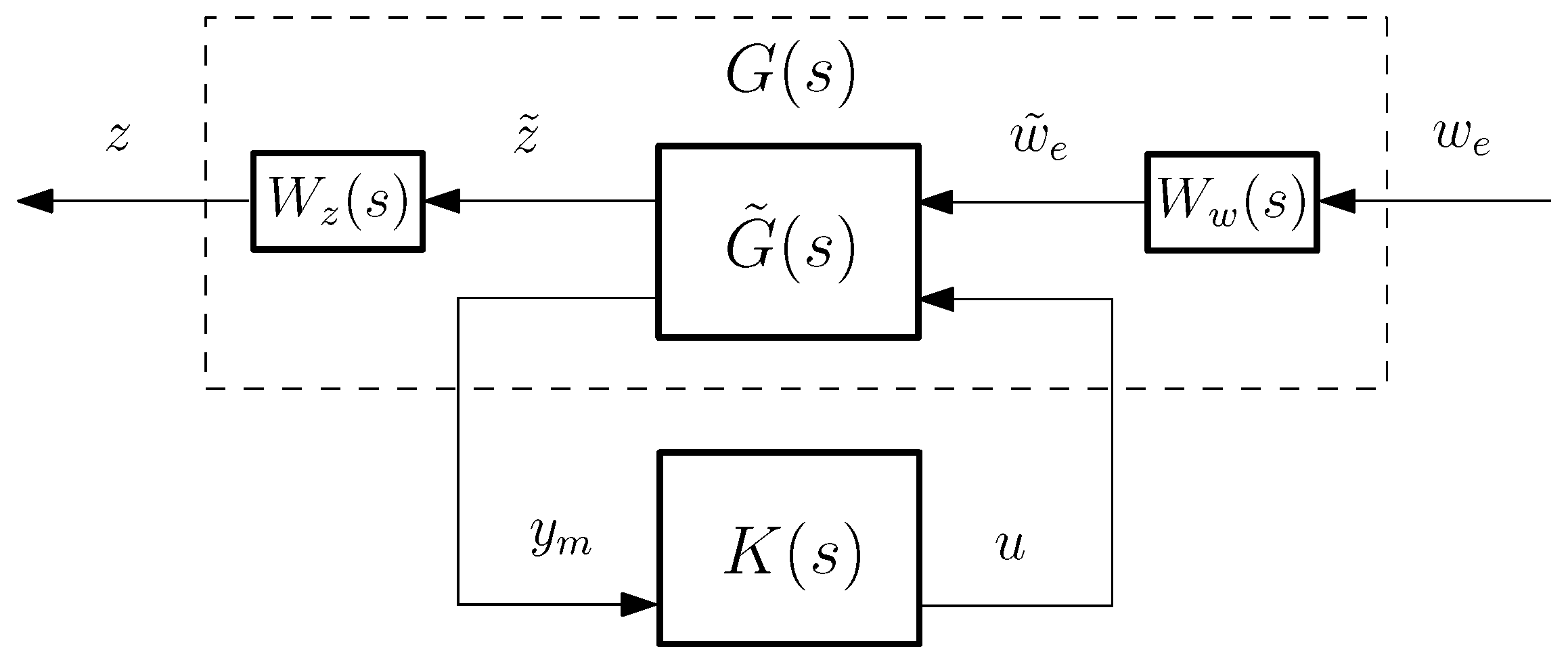
H control is a recommended tool in modern control theory for ensuring the robustness and performance of systems subject to disturbances and model uncertainties. As both a performance and robustness metric, the H norm provides a systematic approach by considering worst-case scenarios in H control synthesis. The H control problem utilizes the H norm to design the controller dynamics that guarantee optimal behavior in the presence of model uncertainties and exogenous inputs. H control synthesis is based on a design framework, which is illustrated in Figure 2.
In the figure, G ( s ) represents the nominal model ( G ˜ ( s ) ) of the system along with performance specifications ( W z ( s ) , W w ( s ) ) and is referred to as the generalized plant. K ( s ) denotes the H controller, designed to satisfy system stability and performance requirements. Additionally, several key signals are present within the design framework. ω e represents the generalized exogenous signals comprising noise (stochastic in nature with known distributions, assumed to be Gaussian and zero-mean) and disturbances (unknown deterministic signals), which are unaffected by the controller. u denotes the controller inputs to the generalized plant, while z is used to define the controlled variables, representing the design specifications to be satisfied by the controller. In general, the goal is for these variables to converge to zero, such as in the case of reference tracking error. Lastly, y m refers to the measured system outputs, which serve as inputs to the controller [35,36].
For the sake of simplifying the H controller design, a generalized mathematical description based on the design framework shown in Figure 2 is required. In state-space representation, the mathematical description is given by
x ˙ G ( t ) = A G x G ( t ) + B G 1 ω e ( t ) + B G 2 u ( t )
z ( t ) = C G 1 x G ( t ) + D G 11 ω e ( t ) + D G 12 u ( t )
y m ( t ) = C G 2 x G ( t ) + D G 12 ω e ( t ) + D G 22 u ( t )
where x G ( t ) represents the generalized plant states, which include the states of the nominal system as well as the states used to describe the performance specifications. u ( t ) is derived from the H controller dynamics. The state-space representation of the controller dynamics is given by
x ˙ k ( t ) = A k x k ( t ) + B k y m ( t )
u ( t ) = C k x k ( t ) + D k y m ( t )
Performance criteria are introduced into the generalized system model through weighting functions, which shape the behavior of the controlled variables and exogenous signals within the closed-loop system [37]. These weighting functions can exhibit different dynamics depending on the design objectives and are described by
z ( t ) = W z ( s ) z ˜ ( t )
ω ˜ e ( t ) = W w ( s ) ω e ( t )
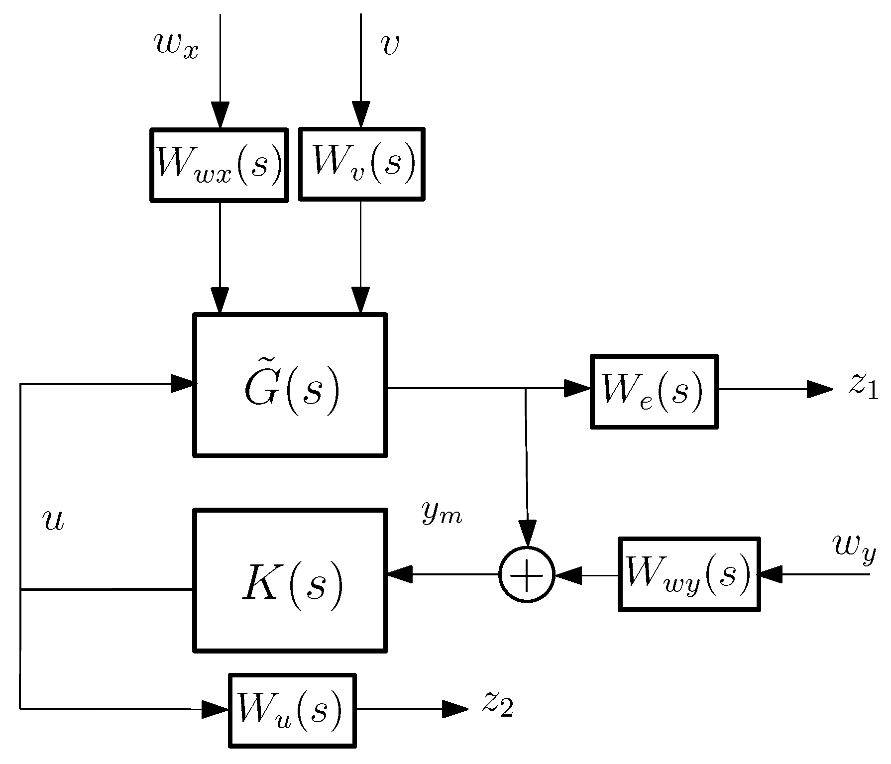
The chosen weighting functions have a direct impact on the designed controller dynamics. Consequently, there is a trade-off between the selected weighting functions and the complexity of the controller. Generally, these weighting functions are utilized to ensure tracking performance and limit the control input of the model by minimizing the noise effect on the controller output. The selected weighting functions, based on the defined objectives, shape the sensitivity function and control sensitivity function of the system. In the detailed H control framework, the relationship between the weighting functions and the corresponding block signals is illustrated in Figure 3.
Typically, W e ( s ) is chosen as a first-order low-pass filter to emphasize reference tracking with high gain at low frequencies while allowing for robust disturbance rejection and noise attenuation with low gain at high frequencies. This is also referred to as the tracking performance weighting function. Additionally, the other weighting function, W u ( s ) , known as the control effort weighting function, is chosen as a first-order high-pass filter [38,39,40,41]. This function discourages large or abrupt control inputs, thereby preventing actuator saturation and promoting gradual, smooth variations in the control signal. At the same time, it minimizes the gain at the relevant frequency ranges, preventing control signals of large magnitude. The remaining weighting functions are utilized to characterize disturbance properties regarding their behavior in the frequency domain. Considering the influence of disturbances on the system characteristics, W w x ( s ) and W w y ( s ) are designed as high-pass filters, whereas W v ( s ) is selected as a low-pass filter [42].
With these characteristics in mind, the main idea is to design an H controller such that the closed-loop system remains stable while minimizing T z ω e ( s ) H . The system T z ω e ( s ) represents the dynamical system that maps the effects of the exogenous signals to the prescribed objective signals.

3.3. Output Feedback H Controller Design via LMI Formulation

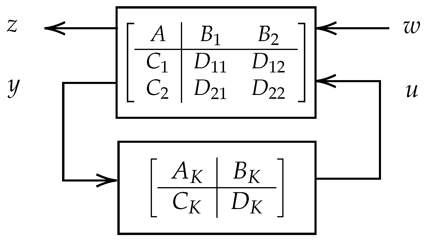
The following part details the LMI-based procedure for designing a dynamic output feedback H controller, including the formulation of the synthesis conditions and the derivation of the associated optimization problem. The design is based on the standard four-block generalized plant configuration, where the closed-loop system is represented in a state-space framework that partitions the exogenous inputs, measured outputs, control inputs, and regulated outputs. This representation facilitates the formulation of the H performance objective as an L 2 -induced gain condition between the disturbance input and the performance output channels, enabling the use of convex LMI constraints to ensure internal stability and robust performance. The four block formation of the closed loop in state-space representation is depicted in Figure 4.
The formulation explicitly captures the interconnection structure between the plant and the controller. In addition to that, the external inputs and outputs are partitioned into the performance and control channels under the given representation. The formulation gives an overview of how the generalized plant comprises nominal dynamics and uncertainty and interfaces with the controller dynamics through the measurable signals, thereby forming a feedback loop amenable to robust control design.
The illustrated configuration is foundational in H control synthesis, where the aim is to minimize the worst-case gain from the exogenous input w to the controlled variable z. As it is given in [16], a set of change of variables yields the following optimization problem formulated using LMIs:
Find X 1 , Y 1 , A n , B n , C n , D n , γ s . t . X 1 I I Y 1 0 A Y 1 + B 2 C n s A + A n + B 2 D n C 2 X 1 A + B n C 2 s B 1 + B 2 D n D 21 X 1 B 1 + B n D 21 C 1 Y 1 + D 12 C n C 1 Y 1 + D 12 C n C 1 + D 12 D n C 2 γ I γ I 0
which is a convex problem (assuming the well-posed condition). The LMI-based formulation ensures that the resulting controller stabilizes the system by achieving the desired H performance level, which is bounded by the scalar γ .
Once an applicable solution to the LMI is obtained for the desired H performance level, the controller dynamics described in the state-space can be recovered using a set of matrix operations given by
D K = I + D K 2 D 22 1 D K 2 , B K = B K 2 I D 22 D K , C K = I D K D 22 C K 2 , A K = A K 2 B K I D 22 D K 1 D 22 C K
where A K 2 B K 2 C K 2 D K 2 is given by
X 2 X 1 B 2 0 I 1 A n B n C n D n X 1 A Y 1 0 0 0 Y 2 0 C 2 Y 1 I 1
for any full-rank X 2 and Y 2 such that the following identity holds:
X 1 X 2 X 2 X 3 = Y 1 Y 2 Y 2 Y 3 1 .
This condition ensures the consistency and invertibility required for the controller reconstruction. Using the optimization problem stated in this section, the robust controller design methodology is detailed in the next section.

3.4. Robust Controller Design

To have a controller that is robust against the bounded changes of the operating point (where the nonlinear system is linearized), the following are implemented:
  • The nonlinear system is linearized around a set of points (all of which are close to the one primary point the system is expected to operate at);
  • For each i t h system, the system T z w e ( i ) is obtained;
  • The following optimization problem is considered:
    min K ( s ) RH max i { 1 , , N } T z w e ( i ) ( s ) H
where the resulting K ( s ) is required to satisfy the well-posed constraint for each of the systems.It is also important to note that the problem given in (24) can be formulated to be a convex optimization problem [43,44,45,46,47,48], and this formulation is similar to the quadratic stability condition given in [19].

4. Control-Based Observer Design Using H  Controller

In this section, the controller-based design is discussed. The concepts of observer and the control-based observer frameworks are introduced, and the necessary formulation is stated in this section.

4.1. Observer Design Concept

The main purpose of control-based observer design is to incorporate the features of the controller into the observer dynamics, thus achieving more accurate and high-performance estimation. The control-based observer design approach suggests solving a control problem rather than directly addressing the observer problem. In this approach, a control law is formulated for the system model to ensure that the real system outputs are closely followed by the model outputs. This method is also used to estimate the unknown system inputs, while the real system states are estimated through the observer dynamics. The performance and accuracy of the state and unknown system input estimations can be enhanced by applying different controller strategies within the observer design. This flexibility offers a broad range of options to shape the observer dynamics based on the chosen control law.
For ensuring robustness and performance in terms of system stability under model uncertainties and disturbances, robust control design techniques are commonly employed, with H being one such method. By following the design steps of the H controller, as detailed in Section 3, the observer dynamics can be shaped by transforming the observer problem into a control problem.
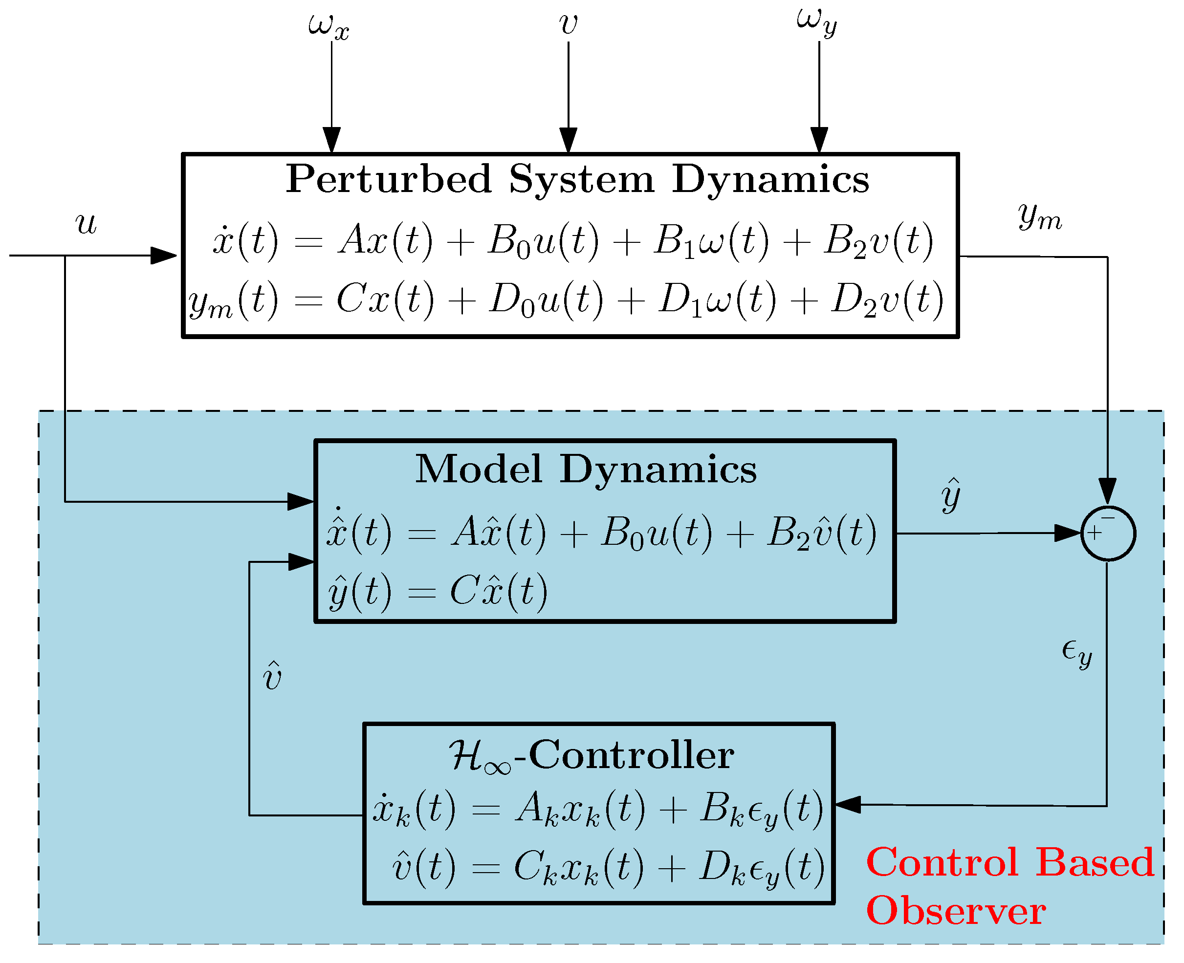
For the control-based observer design, if a system is considered under generalized disturbances and unknown system inputs, the system dynamics are given by
x ˙ ( t ) = A x ( t ) + B 0 u ( t ) + B 1 ω ( t ) + B 2 v ( t )
y ( t ) = C x ( t ) + D 0 u ( t ) + D 1 ω ( t ) + D 2 v ( t )
where x ( t ) R n , u ( t ) R m , and y ( t ) R p represent the system state, known input, and measured outputs, respectively, while ω ( t ) R n + p refers to the disturbance vector, including state noise ( ω x ( t ) R n ) and measurement noise ( ω y ( t ) R p ), and v ( t ) R q represents the unknown system inputs.
The given state-space model describes the real system dynamics. However, the model of the real system may differ from the actual system dynamics due to the inherent nature of system modeling. The state-space representation of the model dynamics is given by
x ^ ˙ ( t ) = A x ^ ( t ) + B 0 u ( t ) + B 2 v ^ ( t )
y ^ ( t ) = C x ^ ( t )
As seen in the given description, the model dynamics do not account for information regarding the exogenous signals, and the model is driven by v ^ ( t ) , which is the output of the H controller used to capture the real system states and unknown inputs.
For the observer design, it is necessary to define an error model, which is obtained by substituting the model dynamics into the real system dynamics. For simplicity, the matrices D 0 and D 2 given in the real system dynamics can be assumed to be zero. Therefore, the error model can be described by
ϵ ˙ x ( t ) = A ϵ x ( t ) B 1 ω ( t ) B 2 v ( t ) + B 2 v ^ ( t )
ϵ y ( t ) = C ϵ x D 1 ω ( t )
The objective of the observer design is to drive the error dynamics to zero, ensuring accurate state and unknown input estimation for the system [49,50]. The error model dynamics are utilized solely to derive the dynamics of the control-based observer under the H control law, with the error dynamics representing the nominal system G ˜ ( s ) as shown in Figure 2. For the analysis of the observer’s state estimation performance and robustness, the system model dynamics are employed in simulation environments or during the observer implementation on hardware. The block diagram, which includes the interconnection between the real system and the control-based observer dynamics, is illustrated in Figure 5.
Before proceeding with the design steps to be used for the observer design, the control-based observer design requires the system to satisfy certain conditions, as outlined below:
  • A , C is observable
  • A , B 2 is controllable
  • r a n k s I A B 2 C 0 = n + p , s C
After satisfying the conditions, the control-based observer design can be achieved by following the H control law synthesis steps outlined in Section 3. Therefore, thanks to the features of the H control law, the observer dynamics can be derived, ensuring robustness and performance in the estimation of the system state and unknown inputs.

4.2. System Linearization

As discussed in Section 3, the H control problem requires a linear time-invariant system for controller synthesis. However, the fixed-wing aircraft exhibits highly nonlinear system characteristics. Therefore, a linearization around a chosen operating point is necessary. Due to the nature of fixed-wing aircraft, there exists a set of operational points corresponding to various flight conditions. For the linearization process, the level-flight condition of the aircraft is considered, with the trim points selected around altitude and indicated airspeed. Thus, the dynamics of the fixed-wing aircraft can be defined as follows:
x ˙ 0 ( t ) = f ( x 0 , u 0 ) = 0
y 0 ( t ) = h ( x 0 , u 0 )
where x 0 , u 0 pair represents the state of the system and inputs at the equilibrium point. As the first step in system linearization, the nonlinear dynamics can be expressed using small perturbation theory, which analyzes the nonlinear dynamics by introducing small perturbations around the equilibrium point:
x ( t ) = x 0 + Δ x ( t )
u ( t ) = u 0 + Δ u ( t )
x ˙ 0 ( t ) + Δ x ˙ ( t ) = f ( x 0 + Δ x ( t ) , u 0 + Δ u ( t ) )
y 0 ( t ) + Δ y ( t ) = h ( x 0 + Δ x ( t ) , u 0 + Δ u ( t ) )
The nonlinear dynamics, defined by the small perturbations and equilibrium point dynamics of the system, can be expressed as follows using a Taylor series expansion, considering only the first-order terms [51,52,53,54,55]:
f ( x 0 + Δ x ( t ) , u 0 + Δ u ( t ) ) f ( x 0 , u 0 ) + f x ( x 0 , u 0 ) Δ x ( t ) + f u ( x 0 , u 0 ) Δ u ( t )
and the output is given by
h ( x 0 + Δ x , u 0 + Δ u ( t ) ) h ( x 0 , u 0 ) + h x ( x 0 , u 0 ) Δ x ( t ) + h u ( x 0 , u 0 ) Δ u ( t )
By considering the simplification, the linearized model can be described in the state-space domain as follows:
Δ x ˙ ( t ) A Δ x ( t ) + B Δ u ( t )
Δ y ( t ) C Δ x ( t ) + D Δ u ( t )
The linearized model of the fixed-wing aircraft can be described by two separate dynamic systems: the lateral and longitudinal dynamics of the aircraft. The control-based observer is designed for the longitudinal dynamics, where the system states and inputs are described as follows [56,57]:
x l o n = [ V , α , q , θ , h ] , u l o n = [ δ t h r u s t , δ e l e v a t o r ]
A control-based observer is formulated to estimate the unmeasurable states and unidentified external inputs of the Apprentice-S model aircraft. The corresponding modeling parameters are summarized in Table 1.
In the table, the presented force and moment derivatives are expressed in a dimensionless form, facilitating their comparison and analysis independent of specific reference units or scaling factors.
The longitudinal dynamics are described for the obtained linearized model of the aircraft at 18.9 m/s (∼37 knots) airspeed and 1000 m (∼3280 ft) altitude trim points. The state-space representation of the longitudinal dynamics is given as follows [58]:
x ˙ l o n ( t ) = 0.1432 3.652 0 9.804 1.3 e 4 0.0549 12.99 0.9418 0 0 0 62.73 5.197 0 0 0 0 1 0 0 0 18.92 0 18.92 0 x l o n ( t ) + 0.7193 2.852 7.7 × 10 4 1.08 0 90.22 0 0 0 0 u l o n ( t )
y l o n ( t ) = 1 0 0 0 0 0 0 0 0 1 x l o n ( t ) + 0 0 u l o n ( t )
As seen in the state-space model, the α , q , θ states cannot be measured. In the observer design problem, the non-measurable states and unknown system inputs are estimated.

5. Simulation Results

In the previous sections, the modeling steps of a fixed-wing aircraft were described. The nonlinear aircraft dynamic model was linearized using small-perturbation theory and Taylor series expansion based on the operational points. The control-based observer was designed by following the H control law synthesis steps to achieve robustness and performance in system state and unknown input estimation.
The simulation environment was created in MATLAB/Simulink, assuming that the system’s unknown inputs are deterministic signals, while the disturbances are characterized by non-deterministic Gaussian signals. This setup facilitates the analysis of the robustness and performance of the observer responses.
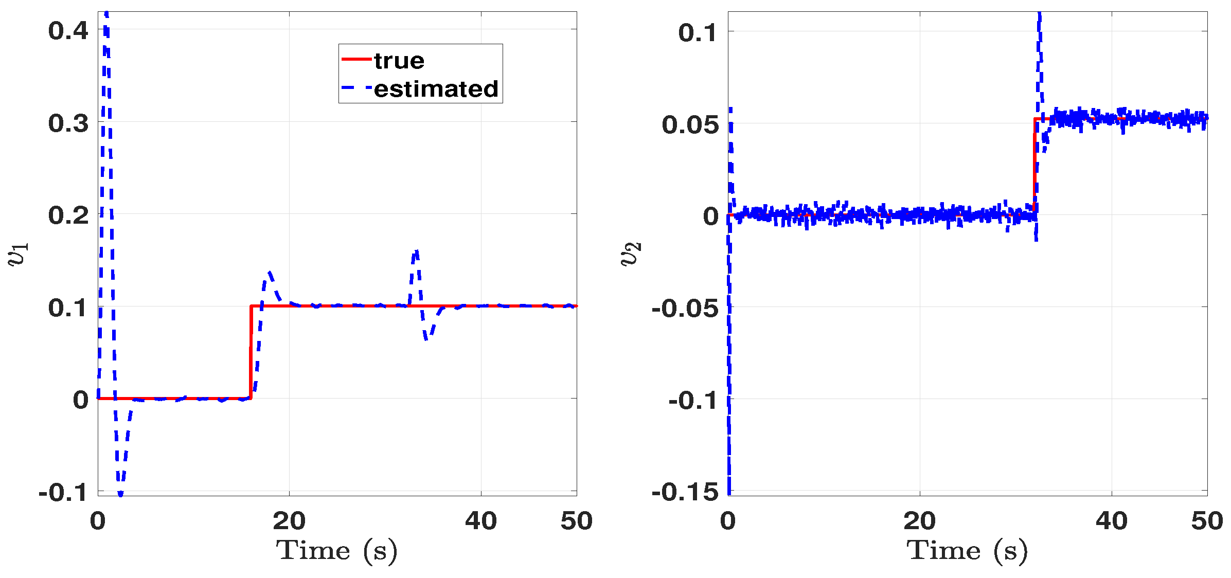
For the estimation of unknown system inputs, the longitudinal dynamics of the fixed-wing aircraft are perturbed by step signals with magnitudes of 0.1 N and 3° through the thrust and elevator control surfaces, respectively. These signals are applied to the system at t = 16 and t = 32 s of the simulation. Additionally, the initial conditions of the system are defined by
x 0 = [ 0.1 0.0346 0.001 0.0524 0.2 ]
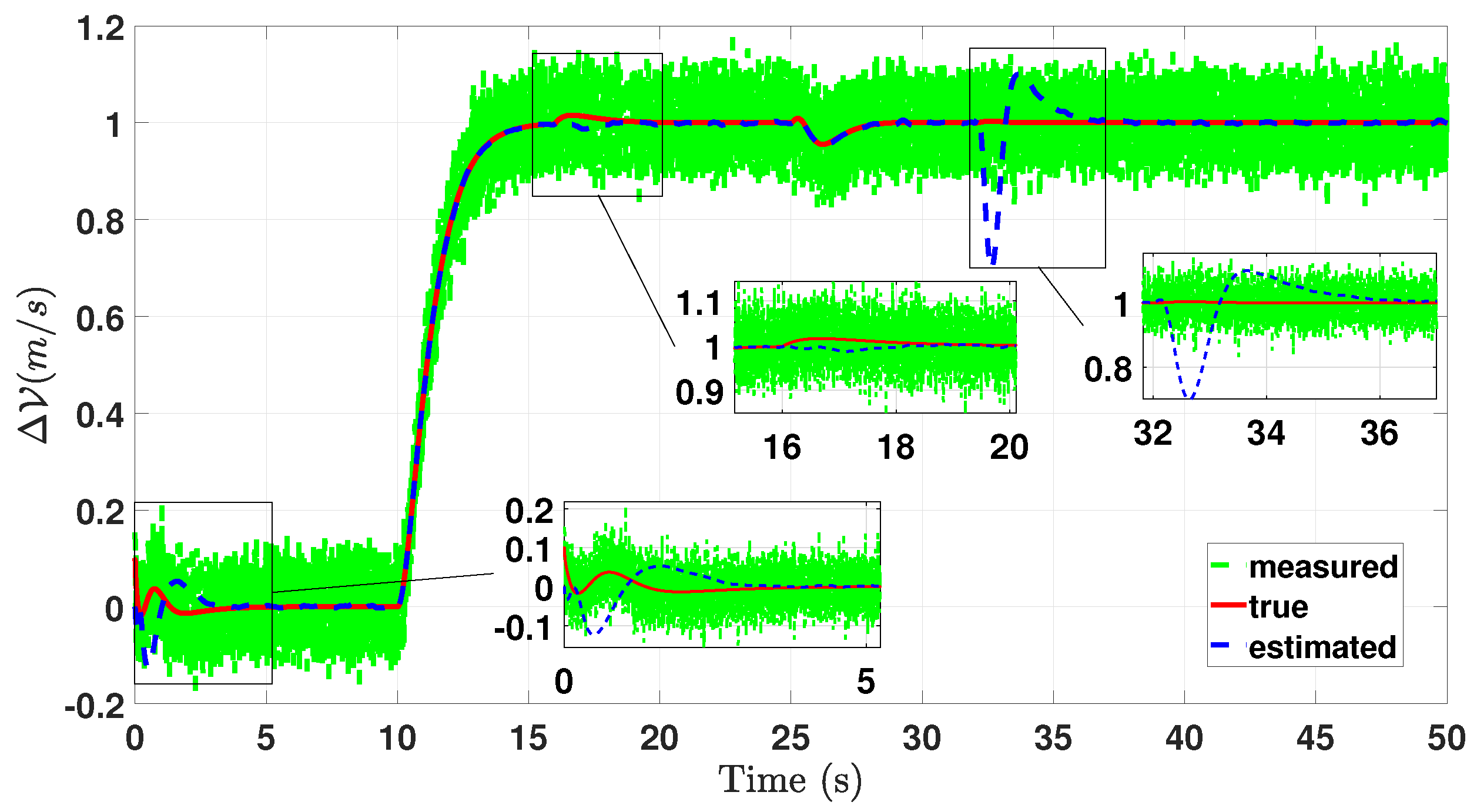
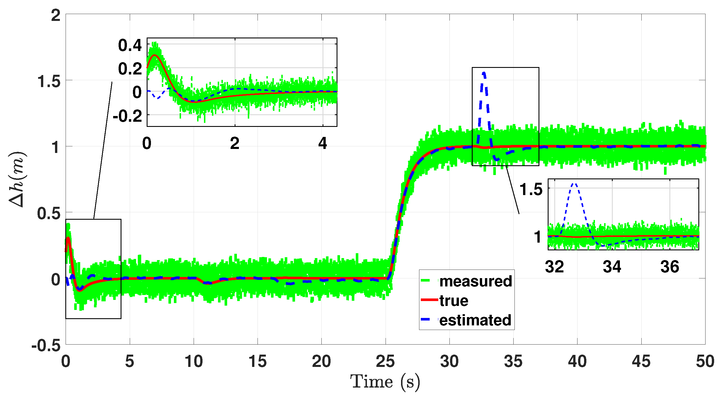
Based on the given settings in the simulation environment, the state estimation performance and robustness are illustrated in Figure 4, Figure 5, Figure 6, Figure 7 and Figure 8, comparing the real system and perturbed system states. As mentioned in the control-based observer design objective, the main purpose is to track the real system outputs by the model output to ensure a desired estimation of the real system state and unknown input. The tracking performance on the real system outputs is illustrated in Figure 6 and Figure 7.
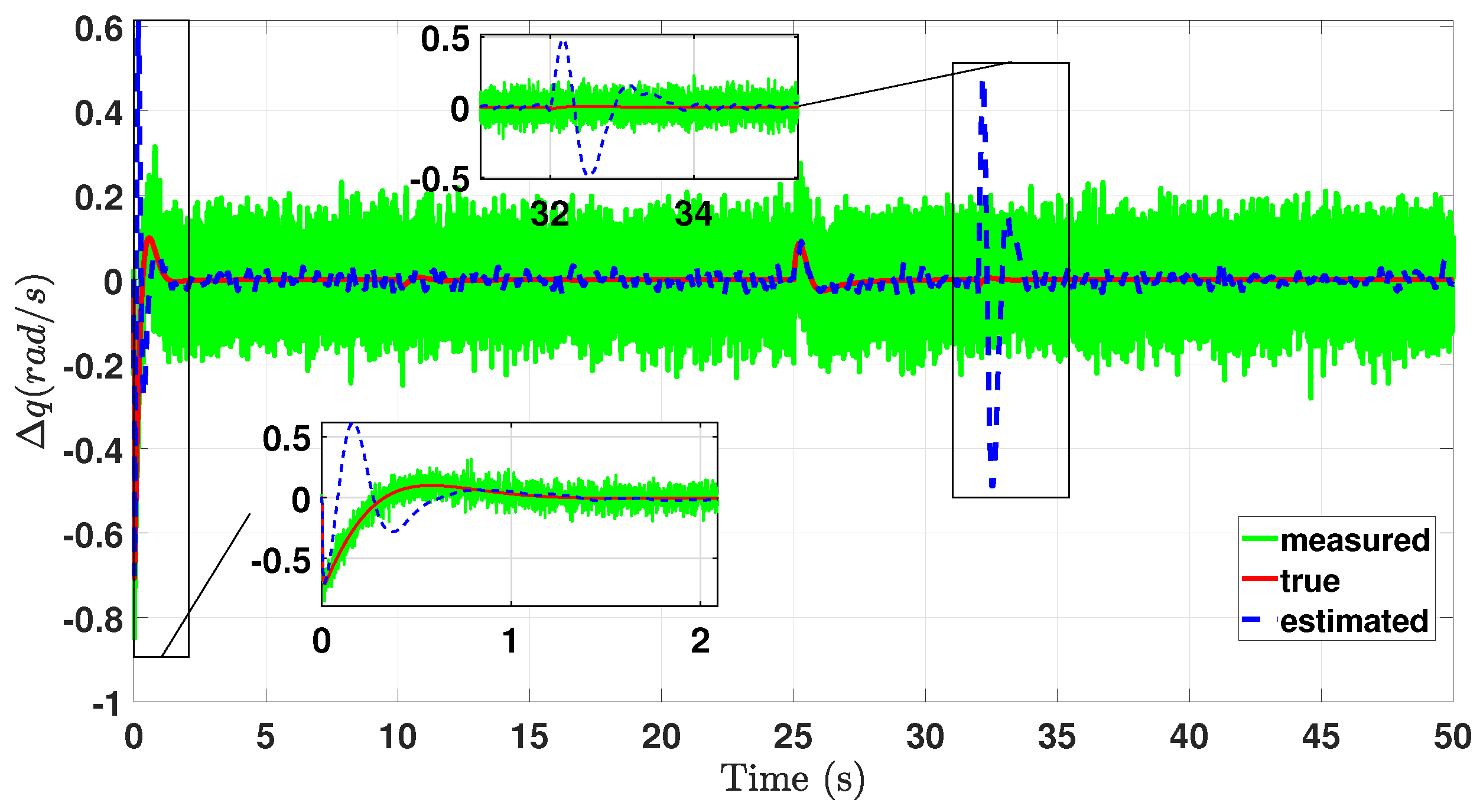
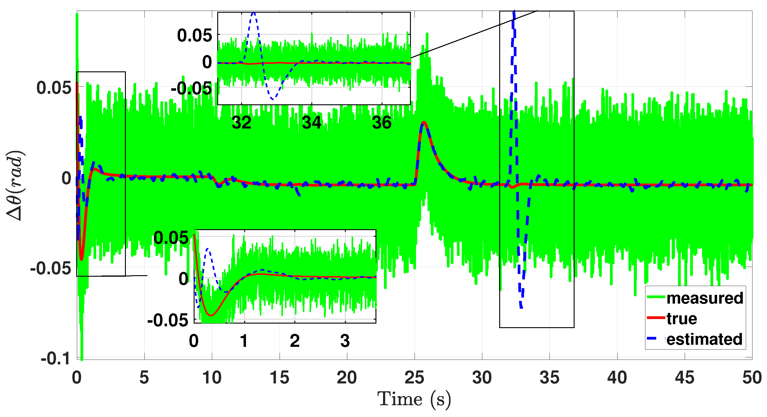
According to the obtained results, as illustrated in the figures, despite the presence of noise in the measured outputs, the observer dynamics effectively track the actual system outputs by mitigating measurement noise. These outputs also correspond to the measurable system states. Given the performance in output tracking, it can be concluded that the estimation of non-measurable states has been successfully achieved. Furthermore, the comparative analysis of the non-measurable states are presented in Figure 8, Figure 9 and Figure 10.
As can be seen in Figure 8, Figure 9 and Figure 10, the control-based observer demonstrates a good performance and robustness in estimating the real system states, even in the presence of disturbances and unknown system inputs. Once the observer captures the system states, it maintains accurate and robust estimation, even when the system dynamics shift to different operating points due to changes in the reference inputs.
In addition to state estimation, another design objective is the estimation of the system’s unknown inputs. Based on the simulation results, the estimation performance and robustness for the unknown inputs are illustrated in Figure 11.
As seen in the graphs, the characteristics of the unknown inputs are effectively captured by the observer dynamics. Typically, the unknown input estimation is analyzed by considering the outputs of the H control law, which are also used to capture the system states. This implies that once the system states are captured by the H control law outputs as a correction term, the outputs are then driven to capture the unknown inputs.
To present the robustness of the observer against the operating point of the aircraft, Monte Carlo simulations have been performed. In each simulation, the airspeed and the altitude (the terms that are used to obtain the linear model) terms take values from the sets [16–19] (m/s)–(∼[31–37] knots) and [800–1200] (m)–(∼[2620–3940] ft), respectively. The resulting estimation error terms for the unmeasured states, measured states, and the unknown inputs are given in Figure 12, Figure 13 and Figure 14, respectively.
As it can be seen in Figure 12, The states that are not measured directly are being estimated accurately for all the cases presented in the Monte Carlo simulations with fast transient response. This is achieved by driving the estimation error terms for the measured signals that are given in Figure 13. Additionally, in the face of system perturbations, the estimation error stays bounded, demonstrating the robustness of the estimator in the face of disturbances and process and measurement noise terms. Finally, the corresponding estimation error for the disturbance terms are given in Figure 14 and can be seen to not be sensitive to the system perturbations. In Figure 12, the maximum root mean square errors (RMSE) associated with the unmeasured state estimations are obtained as 0.0523 rad for the angle of attack, 0.1816 rad/s for the pitch rate, and 0.0846 rad for the pitch angle. Regarding the estimation error deviations of the measured states, illustrated in Figure 13, the worst-case RMSE values are identified as 0.1423 m/s for airspeed and 0.1787 m for altitude. Furthermore, in terms of disturbance estimation, the RMSE values corresponding to the thrust and elevator input signals are found to be 0.1559 and 0.0706, respectively, in Figure 14.
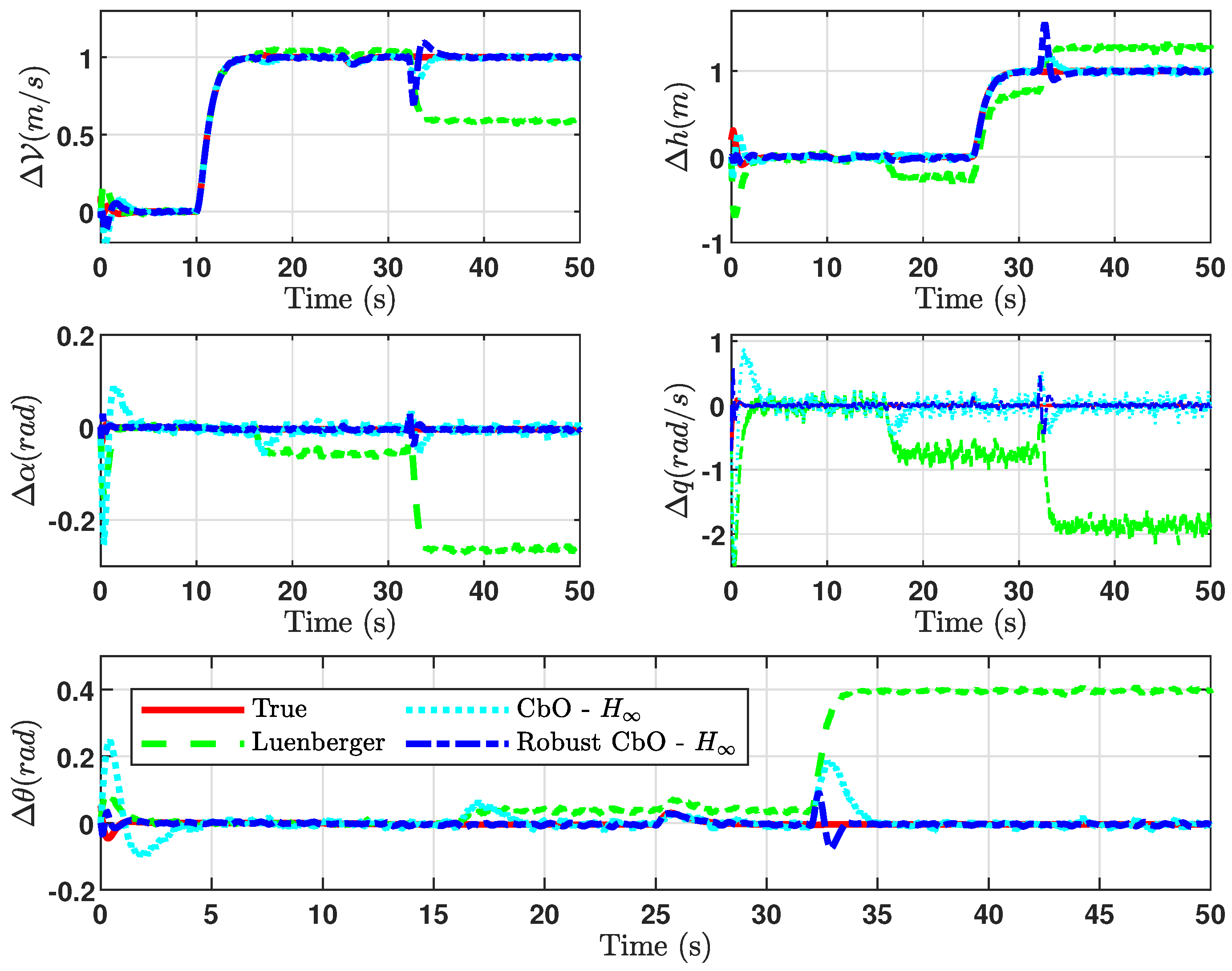
As the final stage of the numerical simulations, to have a better understanding of the performance and robustness characteristics of the CbO framework, the presented CbO approaches are compared against a conventional linear observer, designed for the nominal operating point.
The comparative results are given in Figure 15. In the light of these results, the statistical assessment of the simulations are given in the Table 2. It should be noted that the performance of the conventional linear observer deteriorates as the system operates away from the projected operating point, which is due to the effects of the disturbances that are being considered. As for the robust CbO- H , it can be noted that these changes to the point at which the system operates are embedded in the problem formulation, which causes the performance deterioration to be minimal, as can be seen in the statistical assessment in Table 2.

6. Conclusions

In this study, the mathematical model of a fixed-wing aircraft is derived, and the model is linearized around the operational points to obtain the linearized model of the longitudinal dynamics. The H control problem definition and synthesis steps are outlined, reflecting their relationship with the H norm concept in control systems to ensure robustness and performance. The control-based observer design concept is explained, with guidance provided on how to transfer the stability and robustness features of the control law onto the observer dynamics by approaching the observer problem as a controller design problem. The H control law design steps are applied to derive the observer dynamics for the state and unknown input estimation of a system under state-measurement noise and known inputs in a way that the modeling uncertainties are taken into account, resulting in an observer that is robust to the bounded uncertainties. Finally, the results of the numerical simulations, conducted in the MATLAB/Simulink environment, are presented to demonstrate (i) the observer’s performance around the nominal operating point, (ii) the observer’s robustness to dynamical uncertainties, and (iii) a comparison with a conventional linear observer and interpreted to analyze the benefits of the robust control law on the observer dynamics as shown by improved RMSE in Table 2, focusing on estimation performance and robustness.

Author Contributions

Conceptualization, U.G. and A.S.; formal analysis, A.S.; methodology, U.G.; software, U.G., A.S. and E.S.; supervision, A.S. and C.K.; validation, C.K.; writing—original draft, U.G. and A.S.; writing—review and editing, E.S. and C.K. All authors have read and agreed to the published version of the manuscript.

Funding

This research received no external funding.

Data Availability Statement

Data is contained within the article. The original contributions presented in this study are included in the article.

Acknowledgments

The authors would like to thank TOBB ETU Control Systems Lab (Ankara, The Republic of Turkey) and Prismatic Ltd. Company (Guildford, United Kingdom).

Conflicts of Interest

The authors declare no conflicts of interest.

References

  1. Gunes, U.; Sel, A.; Kasnakoglu, C. Stabilizer Autopilot Design For Fixed Wing UAV Using ODSMC. In Proceedings of the International Conference on System Theory, Control and Computing, Sinaia, Romania, 10–12 October 2018; pp. 740–746. [Google Scholar] [CrossRef]
  2. Sel, A.; Gunes, U.; Kasnakoglu, C. Output Feedback Discrete SMC Design For Quadratic Buck DC-DC Converter. In Proceedings of the 2018 22nd International Conference on System Theory, Control and Computing, Sinaia, Romania, 10–12 October 2018; pp. 728–733. [Google Scholar] [CrossRef]
  3. Sel, A.; Sel, B.; Coskun, U.; Kasnakoglu, C. SOS–Based Nonlinear Observer Design for Simultaneous State and Disturbance Estimation Designed for a PMSM Model. Sustainability 2022, 14, 10650. [Google Scholar] [CrossRef]
  4. Popescu, A.; Besancon, G.; Voda, A. A new robust observer approach for unknown input and state estimation. In Proceedings of the IEEE 2018 European Control Conference (ECC), Limassol, Cyprus, 12–15 June 2018; pp. 1607–1612. [Google Scholar]
  5. Besançon, G.; Munteanu, I. Control strategy for state and input observer design. Syst. Control Lett. 2015, 85, 118–122. [Google Scholar] [CrossRef]
  6. Kim, H.J.; Kim, J.Y.; Kim, J.W.; Kim, S.K.; Na, W.S. Unmanned Aerial Vehicle-Based Automated Path Generation of Rollers for Smart Construction. Electronics 2023, 13, 138. [Google Scholar] [CrossRef]
  7. Feng, J.; Sun, C.; Zhang, J.; Du, Y.; Liu, Z.; Ding, Y. A UAV Path Planning Method in Three-Dimensional Space Based on a Hybrid Gray Wolf Optimization Algorithm. Electronics 2023, 13, 68. [Google Scholar] [CrossRef]
  8. Peng, H.; Liang, M.; Yuan, C.; Ma, Y. EDF-YOLOv5: An Improved Algorithm for Power Transmission Line Defect Detection Based on YOLOv5. Electronics 2023, 13, 148. [Google Scholar] [CrossRef]
  9. Imran, I.H.; Wood, K.; Montazeri, A. Adaptive Control of Unmanned Aerial Vehicles with Varying Payload and Full Parametric Uncertainties. Electronics 2024, 13, 347. [Google Scholar] [CrossRef]
  10. Guerra, T.; Márquez, R.; Kruszewski, A.; Bernal, M. H∞ LMI-Based Observer Design for Nonlinear Systems via Takagi–Sugeno Models with Unmeasured Premise Variables. IEEE Trans. Fuzzy Syst. 2018, 26, 1498–1509. [Google Scholar] [CrossRef]
  11. López-Estrada, F.; de León, H.H.; Estrada-Manzo, V.; Bernal, M. LMI-based fault detection and isolation of nonlinear descriptor systems. In Proceedings of the IEEE International Conference on Fuzzy Systems, Naples, Italy, 9–12 July 2017; pp. 1–5. [Google Scholar] [CrossRef]
  12. Popescu, A.; Besancon, G.; Voda, A. Comparison between different control strategies for estimation purposes using Control-based Observer paradigm. In Proceedings of the International Conference on System Theory, Control and Computing, Sinaia, Romania, 10–12 October 2018; pp. 135–140. [Google Scholar] [CrossRef]
  13. Robles, R.; Sala, A.; Bernal, M.; González, T. Subspace-Based Takagi–Sugeno Modeling for Improved LMI Performance. IEEE Trans. Fuzzy Syst. 2017, 25, 754–767. [Google Scholar] [CrossRef]
  14. Tsukamoto, H.; Chung, S.; Slotine, J. Neural Stochastic Contraction Metrics for Learning-Based Control and Estimation. IEEE Control Syst. Lett. 2021, 5, 1825–1830. [Google Scholar] [CrossRef]
  15. Duan, G.; Yu, H. LMIs in Control Systems; CRC Press: Boca Raton, FL, USA, 2013. [Google Scholar] [CrossRef]
  16. Boyd, S.; Ghaoui, L.; Feron, E.; Balakrishnan, V. Linear Matrix Inequalities in System and Control Theory; Society for Industrial and Applied Mathematics: Philadelphia, PA, USA, 1994. [Google Scholar] [CrossRef]
  17. Miklosovic, R.; Radke, A.; Gao, Z. Discrete implementation and generalization of the extended state observer. In Proceedings of the IEEE 2006 American Control Conference, Minneapolis, MN, USA, 14–16 June 2006; p. 6. [Google Scholar]
  18. Dong, X. Proportional Integral Observer (PIO) Design for Linear Control Systems. Master’s Thesis, University of Rhode Island, Kingston, RI, USA, 2016. [Google Scholar]
  19. Della Rossa, M.; Tanwani, A.; Zaccarian, L. Max–min Lyapunov functions for switched systems and related differential inclusions. Automatica 2020, 120, 109123. [Google Scholar] [CrossRef]
  20. Kurkcu, B.; Kasnakoglu, C.; Efe, M. Disturbance/Uncertainty Estimator Based Integral Sliding-Mode Control. IEEE Trans. Autom. Control 2018, 63, 3940–3947. [Google Scholar] [CrossRef]
  21. Khattar, V.; Ding, Y.; Sel, B.; Lavaei, J.; Jin, M. A CMDP-within-online framework for Meta-Safe Reinforcement Learning. In Proceedings of the International Conference on Learning Representations (ICLR) 2023, Kigali, Rwanda, 1–5 May 2023. [Google Scholar] [CrossRef]
  22. Madhukar, P.; Prasad, L. State Estimation using Extended Kalman Filter and Unscented Kalman Filter. In Proceedings of the IEEE 2020 International Conference on Emerging Trends in Communication, Control and Computing (ICONC3), Lakshmangarh, India, 21–22 February 2020; pp. 1–4. [Google Scholar] [CrossRef]
  23. Wei, X.; Rey, W.; Liu, X. Substation Inspection Robot Location Method Based on Improved Particle Filter. In Proceedings of the IEEE 2024 7th International Conference on Intelligent Robotics and Control Engineering (IRCE), Xi’an, China, 7–9 August 2024; pp. 77–82. [Google Scholar] [CrossRef]
  24. Niu, H.; Ma, Z.; Huang, J.; Lin, G. Ultra-Local Model-Free Predictive Current Control for PMLSM drive systems with Moving Horizon Estimator. In Proceedings of the 2022 IEEE Transportation Electrification Conference and Expo, Asia-Pacific (ITEC Asia-Pacific), Haining, China, 28–31 October 2022; pp. 1–4. [Google Scholar] [CrossRef]
  25. Coskun, U.; Sel, B.; Plaster, B. Magnetic field mapping of inaccessible regions using physics-informed neural networks. Sci. Rep. 2022, 12, 12858. [Google Scholar] [CrossRef]
  26. Stengel, R. Flight Dynamics; Princeton University Press: Princeton, NJ, USA, 2022. [Google Scholar] [CrossRef]
  27. Stevens, B.; Lewis, F.; Johnson, E. Aircraft Control and Simulation: Dynamics, Controls Design, and Autonomous Systems; John Wiley & Sons: Hoboken, NJ, USA, 2015. [Google Scholar] [CrossRef]
  28. Etkin, B.; Reid, L. Dynamics of Flight: Stability and Control, 3rd ed.; John Wiley & Sons: Hoboken, NJ, USA, 1996. [Google Scholar] [CrossRef]
  29. Nelson, R. Flight Stability and Automatic Control, 2nd ed.; McGraw–Hill: Columbus, OH, USA, 1998. [Google Scholar] [CrossRef]
  30. Cook, M. Flight Dynamics Principles: A Linear Systems Approach to Aircraft Stability and Control, 3rd ed.; Butterworth–Heinemann: Oxford, UK, 2013. [Google Scholar] [CrossRef]
  31. Abzug, M.; Larrabee, E. Airplane Stability and Control: A History of the Technologies that Made Aviation Possible, 2nd ed.; Cambridge University Press: Cambridge, UK, 2002. [Google Scholar] [CrossRef]
  32. Phillips, W. Mechanics of Flight, 2nd ed.; John Wiley & Sons: Hoboken, NJ, USA, 2009. [Google Scholar]
  33. Boyd, S.; Vandenberghe, L. Convex Optimization; Cambridge University Press: Cambridge, UK, 2004. [Google Scholar] [CrossRef]
  34. Boyd, S.; Barratt, C. Linear Controller Design: Limits of Performance; Prentice Hall: Hoboken, NJ, USA, 1991. [Google Scholar] [CrossRef]
  35. Basar, T.; Bernhard, P. H∞-Optimal Control and Related Minimax Design Problems: A Dynamic Game Approach, 2nd ed.; Birkhäuser Boston: Cambridge, MA, USA, 2008. [Google Scholar] [CrossRef]
  36. Chen, B. Robust and H∞ Control; Springer: Berlin/Heidelberg, Germany, 2000. [Google Scholar] [CrossRef]
  37. Green, M.; Limebeer, D. Linear Robust Control; Dover Publications: Garden City, NY, USA, 2013. [Google Scholar]
  38. Nasihati, F.; Kiani, M.; Pourtakdoust, S. Satellite pose estimation using Earth radiation modeled by artificial neural networks. Adv. Space Res. 2022, 70, 2195–2207. [Google Scholar] [CrossRef]
  39. Pourtakdoust, S.; Mehrjardi, M.; Hajkarim, M.; Nasihati, F. Advanced fault detection and diagnosis in spacecraft attitude control systems: Current state and challenges. Proc. Inst. Mech. Eng. Part G J. Aerosp. Eng. 2023, 237, 2679–2699. [Google Scholar] [CrossRef]
  40. Nasihati, F.; Kiani, M.; Pourtakdoust, S. Autonomous temperature-based orbit estimation. Aerosp. Sci. Technol. 2019, 86, 671–682. [Google Scholar] [CrossRef]
  41. Nasihati, F.; Kiani, M.; Pourtakdoust, S. On-line orbit and albedo estimation using a strong tracking algorithm via satellite surface temperature data. IEEE Trans. Aerosp. Electron. Syst. 2020, 57, 1443–1454. [Google Scholar] [CrossRef]
  42. Zhou, K.; Doyle, J.; Glover, K. Robust and Optimal Control; Prentice Halll: Hoboken, NJ, USA, 1995. [Google Scholar]
  43. Tawaha, A.; Kaushik, H.; Sel, B.; Jia, R.; Jin, M. Decision-Focused Learning for Inverse Noncooperative Games: Generalization Bounds and Convergence Analysis. IFAC-PapersOnLine 2023, 56, 9336–9341. [Google Scholar] [CrossRef]
  44. Sel, B.; Tawaha, A.; Ding, Y.; Jia, R.; Ji, B.; Lavaei, J.; Jin, M. Learning-to-Learn to Guide Random Search: Derivative-Free Meta Blackbox Optimization on Manifold. In Proceedings of the The 5th Annual Learning for Dynamics and Control Conference, PMLR (Proceedings of Machine Learning Research), Philadelphia, PA, USA, 15–16 June 2023; Matni, N., Morari, M., Pappas, G.J., Eds.; Volume 211, pp. 38–50. [Google Scholar]
  45. Jin, M.; Khattar, V.; Kaushik, H.; Sel, B.; Jia, R. On Solution Functions of Optimization: Universal Approximation and Covering Number Bounds. Proc. AAAI Conf. Artif. Intell. 2023, 37, 8123–8131. [Google Scholar] [CrossRef]
  46. Gu, S.; Sel, B.; Ding, Y.; Wang, L.; Lin, Q.; Jin, M.; Knoll, A. Balance Reward and Safety Optimization for Safe Reinforcement Learning: A Perspective of Gradient Manipulation. Proc. AAAI Conf. Artif. Intell. 2024, 38, 21099–21106. [Google Scholar] [CrossRef]
  47. Gu, S.; Sel, B.; Ding, Y.; Wang, L.; Lin, Q.; Knoll, A.; Jin, M. Safe and Balanced: A Framework for Constrained Multi-Objective Reinforcement Learning. IEEE Trans. Pattern Anal. Mach. Intell. 2025, 47, 3322–3331. [Google Scholar] [CrossRef] [PubMed]
  48. Jin, M.; Sel, B.; Hardeep, F.; Yin, W. Democratizing Energy Management with LLM-Assisted Optimization Autoformalism. In In Proceedings of the 2024 IEEE International Conference on Communications, Control, and Computing Technologies for Smart Grids (SmartGridComm), Oslo, Norway, 17–20 September 2024; pp. 258–263. [Google Scholar] [CrossRef]
  49. Duan, G. Generalized Sylvester Equations; CRC Press: Boca Raton, FL, USA, 2020. [Google Scholar] [CrossRef]
  50. Duan, G. Analysis and Design of Descriptor Linear Systems, 2010 ed.; Springer: Berlin/Heidelberg, Germany, 2010. [Google Scholar] [CrossRef]
  51. Khalil, H. Nonlinear Control, 1st ed.; Pearson Education: Hoboken, NJ, USA, 2015. [Google Scholar]
  52. Khalil, H. Control Systems: An Introduction; Michigan Publishing Services: Ann Arbor, MI, USA, 2023. [Google Scholar] [CrossRef]
  53. Durham, W. Aircraft Flight Dynamics and Control, 1st ed.; John Wiley & Sons: Hoboken, NJ, USA, 2013. [Google Scholar]
  54. Gunes, U.; Sel, A.; Kasnakoglu, C.; Kaynak, U. Output Feedback Sliding Mode Control of a Fixed-Wing UAV Under Rudder Loss. In Proceedings of the AIAA SCITECH Forum. American Institute of Aeronautics and Astronautics, San Diego, CA, USA, 7–11 January 2019. [Google Scholar] [CrossRef]
  55. Gunes, U.; Sel, A.; Sel, B.; Kasnakoglu, C. Dynamic Modeling and Trajectory Tracking of a Quadcopter via Linear and Backstepping Controller. In Proceedings of the AIAA SCITECH Forum. American Institute of Aeronautics and Astronautics, National Harbor, MD, USA/Online, 23–27 January 2023. [Google Scholar] [CrossRef]
  56. Khalil, H. High-Gain Observers in Nonlinear Feedback Control; Society for Industrial and Applied Mathematics: Philadelphia, PA, USA, 2017; Volume 31. [Google Scholar] [CrossRef]
  57. Bayrak, A.; Kurkcu, B.; Efe, M. A New Adaptive Disturbance/Uncertainty Estimator Based Control Scheme For LTI Systems. IEEE Access 2022, 10, 106849–106858. [Google Scholar] [CrossRef]
  58. Zipfel, P. Modeling and Simulation of Aerospace Vehicle Dynamics, 3rd ed.; American Institute of Aeronautics and Astronautics: Reston, VA, USA, 2014. [Google Scholar]
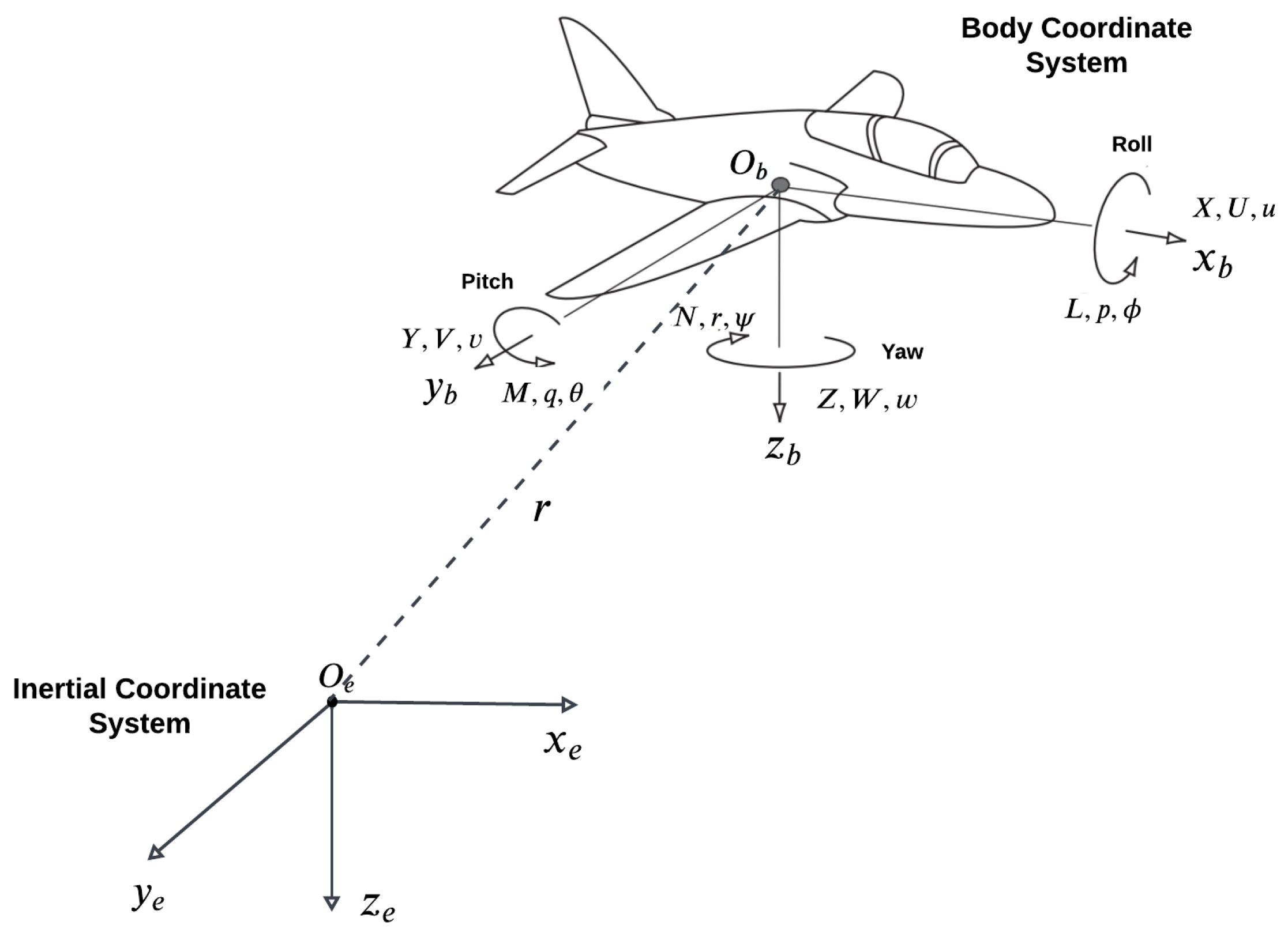
Figure 1. Orientation of the aircraft body-axis system relative to the inertial frame.
Electronics 14 03555 g001
Figure 2. H design framework.
Electronics 14 03555 g002
Figure 3. Detailed H design framework with the weighting functions.
Electronics 14 03555 g003
Figure 4. State-space representation of the closed-loop system in four-block formation.
Electronics 14 03555 g004
Figure 5. The block diagram of the perturbed system dynamics with control-based observer dynamics.
Electronics 14 03555 g005
Figure 6. The comparative analysis for the real, measured and estimated indicated airspeed.
Electronics 14 03555 g006
Figure 7. The comparative analysis for the real, measured and estimated altitude.
Electronics 14 03555 g007
Figure 8. The comparative analysis for the real, perturbed system and observer response on angle of attack.
Electronics 14 03555 g008
Figure 9. The comparative analysis for the real, perturbed system and observer response on pitch rate.
Electronics 14 03555 g009
Figure 10. The comparative analysis for the real, perturbed system and observer response on pitch angle.
Electronics 14 03555 g010
Figure 11. Estimation of unknown inputs.
Electronics 14 03555 g011
Figure 12. Estimation errors of the unmeasured states in Monte Carlo simulations.
Electronics 14 03555 g012
Figure 13. Estimation errors of the measured states in Monte Carlo simulations.
Electronics 14 03555 g013
Figure 14. Estimation errors of the unknown inputs in Monte Carlo simulations.
Electronics 14 03555 g014
Figure 15. The comparative analysis of the observer’s state estimation performance for airspeed ( V ) , altitude ( h ) , angle of attack ( α ) , pitch rate ( q ) , and pitch angle ( θ ) .
Electronics 14 03555 g015
Table 1. The Modeling Parameters of Apprentice-S Model Aircraft.
Parameter SetVariableValue
Geometry and Mass [ c ¯ b ] ( m ) S ( m 2 )
[ I x x I y y I z z ] ( kg · m 2 )
[ I x y I x z I y z ] ( kg · m 2 ) m ( kg )
[ 0.225    1.477 ]    0.332
[ 0.48    0.2109    0.1083 ]
[ 0    0    0 ]    1.39
Aerodynamic
Drag Derivatives
C D 0 C D α C D q
C D δ e C D i h
0.031    0.13    0
0.06    0
Aerodynamic
Y-Force Derivatives
C Y 0 C Y β C Y p
C Y r C Y δ α C Y δ r
0    −0.31    −0.037
0.21    0    0.187
Aerodynamic
Lift Derivatives
C L 0 C L α C L q
C L δ e C L i h
0.31   5.143    3.9
0.43    0
Aerodynamic
X-Moment Derivatives
C l 0 C l β C l p
C l r C l δ a C l δ r
0    −0.089    −0.47
0.096    −0.178    0.0147
Aerodynamic
Y-Moment Derivatives
C m 0 C m α C m q
C m δ e C m i h
−0.015    −0.89    −12.4
−1.28    0
Aerodynamic
Z-Moment Derivatives
C n 0 C n β C n p
C n r C n δ a C n δ r
0    0.065    −0.03
−0.099    −0.053    0.0657
Table 2. Comparison of estimation results with root mean square error (RMSE).
Observer Type ( V V ^ ) ( α α ^ ) ( q q ^ ) ( θ θ ^ ) ( h h ^ )
Luenberger 3.98 × 10 1 3.29 × 10 1 9.69 × 10 1 3.94 × 10 1 4.38 × 10 1
CbO- H 1.26 × 10 1 1.13 × 10 1 3.58 × 10 1 1.36 × 10 1 1.7 × 10 1
Robust CbO- H 1.14 × 10 1 4.23 × 10 2 1.66 × 10 1 6.24 × 10 2 1.49 × 10 1
Disclaimer/Publisher’s Note: The statements, opinions and data contained in all publications are solely those of the individual author(s) and contributor(s) and not of MDPI and/or the editor(s). MDPI and/or the editor(s) disclaim responsibility for any injury to people or property resulting from any ideas, methods, instructions or products referred to in the content.