Hyperspectral Image Classification Using a Spectral-Cube Gated Harmony Network

Abstract

In recent years, hybrid models that integrate Convolutional Neural Networks (CNNs) with Vision Transformers (ViTs) have achieved significant improvements in hyperspectral image classification (HSIC). Nevertheless, their complex architectures often lead to computational redundancy and inefficient feature fusion, particularly struggling to balance global modeling and local detail extraction in high-dimensional spectral data. To solve these issues, this paper proposes a Spectral-Cube Gated Harmony Network (SCGHN) that achieves efficient spectral–spatial joint feature modeling through a dynamic gating mechanism and hierarchical feature decoupling strategy. There are three primary innovative contributions of this paper as follows: Firstly, we design a Spectral Cooperative Parallel Convolution (SCPC) module that combines dynamic gating in the spectral dimension and spatial deformable convolution. This module adopts a dual-path parallel architecture that adaptively enhances key bands and captures local textures, thereby significantly improving feature discriminability at mixed ground object boundaries. Secondly, we propose a Dual-Gated Fusion (DGF) module that achieves cross-scale contextual complementarity through group convolution and lightweight attention, thereby enhancing hierarchical semantic representations with significantly lower computational complexity. Finally, by means of the coordinated design of 3D convolution and lightweight classification decision blocks, we construct an end-to-end lightweight framework that effectively alleviates the structural redundancy issues of traditional hybrid models. Extensive experiments on three standard hyperspectral datasets reveal that our SCGHN requires fewer parameters and exhibits lower computational complexity as compared with some existing HSIC methods.

1. Introduction

Hyperspectral image classification (HSIC) is regarded as a core technology in the field of remote sensing [1]. Its primary objective is to classify and identify ground objects by analyzing their spectral signatures across hundreds of contiguous narrow bands. HSIC has provided important support for critical applications including agricultural monitoring [2,3,4,5], environmental assessment [6,7], mineral exploration [8], military target recognition [9,10], urban planning [11] and medical image analysis [12]. With the intensification of climate change, HSIC’s capability of dynamic surface monitoring has become a critical decision-making tool for ecological governance and disaster early warning.

During the last few decades, sustained improvements in the spatial–spectral resolution of hyperspectral sensors have triggered an exponential increase in data dimensionality. Furthermore, constrained by the high cost of acquiring labeled samples and significant spectral redundancy, how to extract robust spectral–spatial joint features from high-dimensional images and achieve efficient classification has emerged as a core research challenge [13]. To solve this issue, researchers have proposed various feature extraction and classification methods, which can be roughly categorized into two types: shallow models based on handcrafted features and data-driven deep learning methods.

Early studies predominantly relied on handcrafted feature extractors. These handcrafted methods mainly included Support Vector Machine (SVM) [14,15], Mathematical Morphological Profile (MP) [16], statistical classification [17], decision tree [18], K-nearest neighbor (KNN) [19], Gabor filter [20], and random field [21] methods. Overall, although traditional methods exhibit high computational efficiency and simple principles, they suffer from limitations in feature representation capability and inadequate generalization performance. Furthermore, computational complexity remains a critical challenge requiring urgent resolution. For example, the Extended Multi-Attribute Profile (EMAP) [22] can enhance spatial feature representation, but its computational complexity grows exponentially with the number of attributes.

Deep learning-based hyperspectral image classification methods primarily include Convolutional Neural Networks (CNNs) and Vision Transformers (ViTs). Using an end-to-end feature representation learning mechanism, these approaches significantly enhance classification accuracy and feature representation capability [23,24].

With the rise of deep learning, CNNs have become the dominant framework for HSIC by using a local receptive field and weight-sharing mechanism. The 1D-CNN [25] approach directly processes spectral vectors, primarily mining inter-band variation trends along the spectral dimension. Lee et al. [26] proposed a 2D-CNN framework to unite the spatial and spectral features of HSI. Chen et al. [27] proposed a 3D-CNN framework that extracts spectral–spatial joint features through three-dimensional convolutional kernels. SSRN [28] introduced residual connections to mitigate gradient vanishing. With the development of CNN-based models, issues of structural complexity and excessive parameters became critical challenges. Therefore, lightweight CNNs have become a research hotspot. MobileNet [29] employs depth-wise separable convolutions to reduce the parameter count. Roy et al. [30] proposed a lightweight improvement scheme termed the HybridSN model, which balances computational efficiency through a hierarchical architecture alternating 3D and 2D convolutions. Overall, although lightweight CNNs significantly reduce computational costs, their local modeling mechanisms remain inadequate for the global feature requirements in HSI, in particular, causing spatial-dimensional information loss when processing cubic samples.

In the field of HSIC, CNN-based models exhibit certain limitations in global modeling. Transformer adopts self-attention mechanisms to break through the locality constraints of CNNs and offers new ideas for global feature modeling. The ITF [31] approach integrates the self-attention mechanism of Transformer architectures with implicit neural representation (INR) technology, and directly models spectral–spatial joint features through multi-head self-attention mechanisms. The PT-Former [32] method combines position-aware embedding modules and temporal difference-aware modules to effectively model spatial and temporal relationships in bi-temporal remote sensing images. However, Transformer-only architectures face challenges when processing large-scale hyperspectral scenes due to their computational complexity being quadratically related to sequence length. CNN-Transformer hybrid models have been extensively adopted to combine local and global information in hyperspectral images (HSIs). SSFTT [33] combines 3D convolutions with Gaussian-weighted tokenization, and utilizes Transformer encoders to model high-level semantic relationships. The GSC-ViT [34] method employs group separable convolutions and lightweight Transformers for extraction of the spectral and spatial features from HSI.

Although these CNN-Transformer hybrid models have achieved progress in hyperspectral image feature extraction and modeling, several critical issues persist. From an architectural perspective, the extensive repetition of convolutional layers and multi-head attention mechanisms leads to a significant increase in the parameter count. During feature fusion stages, interference between different modal features results in inefficient fusion processes, thereby hindering the full exploitation of the hybrid CNN-Transformer model’s advantages.

A dynamic gating strategy has been applied in certain models as a mechanism capable of effectively filtering and regulating information flow; this strategy offers new ideas to address the aforementioned problems. In related studies, Chang et al. [35] proposed an unsupervised multi-view graph contrastive feature learning method, which employs gating mechanisms to assign weights to different views during the multi-view construction phase. Wang et al. [36] proposed a method that combine adaptive gating mechanisms and learnable Transformers to address joint classification of hyperspectral and LiDAR data; this method can dynamically adjust feature weights through an adaptive gating fusion module. Distante et al. [37] proposed a “Gate-Shift-Fuse” mechanism, which utilizes learnable gating weights to dynamically regulate feature interactions between CNN and Transformer branches, while enhancing local–global feature fusion via spatial shift operations.

To effectively address the existing challenges of high computational complexity, parameter redundancy, and low feature fusion efficiency in CNN-Transformer hybrid models, we propose a novel lightweight model referred to as the “Spectral-Cube Gated Harmony Network ” (hereafter dubbed SCGHN). This model ingeniously integrates a CNN with a dynamic gating mechanism. On the one hand, it uses the CNN to efficiently extract local features, thereby reducing parameter redundancy. On the other hand, it uses a dynamic gating mechanism to adaptively filter and fuse spectral–spatial features, thereby enhancing feature fusion efficiency while reducing computational load. The main contributions of our work are summarized as follows:

• We construct a lightweight model integrating a CNN with dynamic gating mechanisms, and propose a Spectral Cooperative Parallel Convolution (SCPC) module to replace the traditional 2D-CNN. SCPC employs a multi-branch interaction mechanism and achieves efficient decoupling-complementarity of spectral–spatial features through a dual-path parallel architecture. Consequently, SCPC reduces the parameter count while enhancing feature discriminability in mixed land-cover boundaries, and effectively addresses the dimensional coupling limitations of traditional single-path methods;
• We design a Dual-Gated Fusion (DGF) module. This module adopts a multi-stage gating aggregation mechanism that decomposes feature processing into local and global branches. The local branch captures neighborhood features through grouped convolution. The global branch establishes long-range spatial correlations through a lightweight attention mechanism. Finally, cross-scale feature complementarity is achieved through adaptive weight fusion, reducing computational overhead while preserving multi-level information;
• SCGHN achieves hierarchical integration of local details and cross-channel contextual information by combining 3D convolution, SCPC and DGF. Therefore, this model significantly enhances the high-level semantic representation capability of HSI while maintaining computational efficiency.

Comprehensive experiments were implemented in three credible hyperspectral datasets. The results indicate that SCGHN achieves the minimum training cost. Compared with several advanced CNN and ViT models previously utilized for HSI classification, our proposed model attains higher classification accuracy with fewer training samples required.

The remainder of this paper is structured as follows. Section 2 elaborates the architectural design of the proposed SCGHN model. Section 3 describes rigorous experimental verifications on the SCGHN model. Section 4 concludes the paper and outlines some potential directions for future research.

2. Proposed Method

In this section, we describe the proposed SCGHN model. Firstly, we present the overall architecture of SCGHN and its workflow for HSIC. Secondly, we consider the design motivations of several key components in the SCGHN architecture.

2.1. Architecture of SCGHN Model

The overall framework of SCGHN is illustrated in Figure 1 and can be divided into four key components: the first is the Multimodal Input Preprocessing (MIPP) module, the second is the Spectral Cooperative Parallel Convolution (SCPC) module, the third is the Dual-Gated Fusion (DGF) module, and the last component is the Lightweight Classification Decision (LCD) module.

In the SCGHN framework, the input data are represented as a 3D spectral cube whose channel dimension varies across datasets. We employ an MIPP module to perform spectral dimension standardization for subsequent feature grouping. The MIPP module adopts 3D convolution to extract spatial–spectral joint features from the input data, achieving preliminary dimensionality reduction. Subsequently, the SCPC module integrates grouped depth-wise convolution and spatial-channel reconstruction convolution, and halves the channel dimension progressively through hierarchical compression to realize extraction of local spectral–spatial joint features. The DGF module then captures cross-scale spatial dependencies through a multi-scale gating mechanism and dynamically fuses spectral-channel information. After multi-stage feature aggregation, SCGHN compresses the feature maps to a 1 × 1 spatial resolution through global average pooling in the LCD module. Ultimately, the compressed features are vectorized and inputted into a fully connected layer-based classifier to generate classification results.

2.2. Multimodal Input Preprocessing (MIPP) Module

The Multimodal Input Preprocessing (MIPP) module is the initial feature extraction unit of SCGHN, which achieves spectral–spatial joint feature extraction of hyperspectral data through 3D convolution. The module is designed to deal with the dual challenges of spectral redundancy and complex spatial structures in hyperspectral imagery (HSI).

The 3D convolutional layer is the core component of MIPP. Its mathematical expression is shown in Equation (1):

$$Y=X\times W+b$$

(1)

where $X\in {\mathbb{R}}^{B\times C\times D\times H\times W}$ is the hyperspectral cube (B is the batch size, C is the input channel, D is the spectral band, H and W denote the spatial dimension). $W\in {\mathbb{R}}^{k_c\times k_h\times k_w\times k_d\times O}$ is the 3D convolution kernel (O is the output channel) and b is the bias term.

Through sliding window operations, this layer maps each 3 × 3 × 3 neighborhood of the input data into an 8-dimensional feature vector, effectively capturing local spectral–spatial features.

Subsequently, this module introduces 3D batch normalization to alleviate the gradient vanishing problem and accelerate training convergence, as illustrated in Equation (2):

$$Y=\gamma ·{\displaystyle \frac{X-{\mu }_B}{\sqrt{{\sigma }_B^2+ϵ}}}+\beta$$

(2)

where ${\mu }_B$ and ${\sigma }_B^2$ denote the mean and variance of the current batch data. $\gamma$ and $\beta$ denote the learnable scale and shift parameters. $ϵ$ is a small constant to prevent division by zero.

This operation stabilizes the feature distribution within the sensitive region of the activation function through normalization, thereby enhancing the model’s generalization capability.

Finally, the ReLU activation function is employed to introduce nonlinear transformation, as illustrated in Equation (3):

$$Y=max\left(0,X\right)$$

(3)

This function effectively mitigates the gradient explosion problem by suppressing negative feature responses while maintaining computational efficiency. Compared to traditional Sigmoid/Tanh functions, the sparsity property of ReLU is more suitable for the high-dimensional characteristics of hyperspectral data.

Two primary reasons motivate our adoption of this module for initial feature extraction. First, the hierarchical 3D convolution achieves multimodal alignment in a parameter-efficient manner, where each kernel requires only a minimal number of parameters, significantly reducing computational costs compared to conventional stacked 2D convolution schemes. Second, the cubic convolution kernel adaptively fuses spectral–spatial features while preserving geometric correlations, thereby establishing the foundation for subsequent parallel cooperative processing through a grouped convolution mechanism.

2.3. Spectral Cooperative Parallel Convolution (SCPC) Module

To address the insufficient collaborative modeling of local details and global context in traditional CNN–Transformer hybrid models for hyperspectral images, we propose the Spectral Cooperative Parallel Convolution (SCPC) module. This module serves as the central feature extraction component of the SCGHN architecture, aiming to efficiently capture the spectral–spatial joint features of HSI through the synergistic interaction of grouped convolution and spatial-channel reconstruction convolution. The module achieves redundant feature suppression and feature representation enhancement through the following structural designs. The framework of SCPC is illustrated in Figure 2.

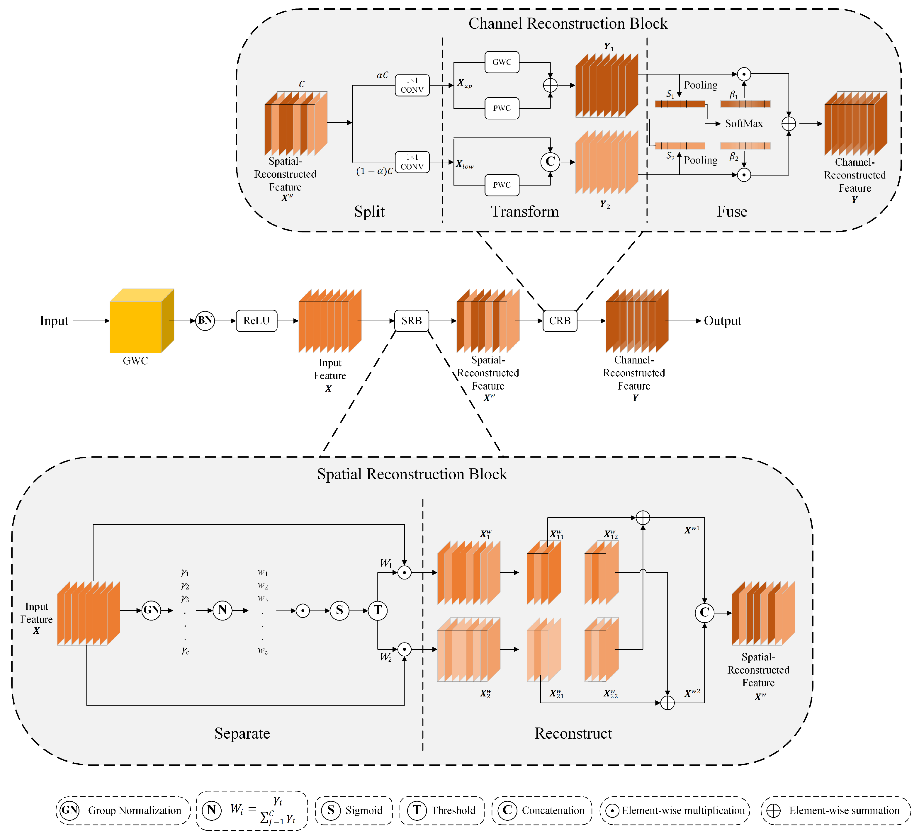
As shown in Figure 2, the Group-Wise Convolution (GWC) layer serves as the initial operation of the SCPC module, reducing inter-channel redundancy through sparse connectivity. Compared to standard convolution, the hierarchical convolution enhances the collaborative modeling capability of local details and global context by decomposing multi-scale feature extraction in spectral and spatial dimensions while reducing parameter quantities. The mathematical formulation of the grouped convolution operation is given in Equation (4):

$$Y=GWC\left(X,W,g\right)=\sum _{i=1}^g{W}_i\ast X_i$$

(4)

where $X\in {\mathbb{R}}^{B\times C\times H\times W}$ is the input feature map, $W\in {\mathbb{R}}^{{\displaystyle \frac{C}{g}}\times k\times k\times C}$ is the grouped convolution kernel. $X_i\in {\mathbb{R}}^{B\times {\displaystyle \frac{C}{g}}\times H\times W}$ is the input of the i-th group, $W_i\in {\mathbb{R}}^{{\displaystyle \frac{C}{g}}\times 3\times 3\times {\displaystyle \frac{C}{g}}}$ is the kernel of the i-th group, “ * ” denotes the convolution operation.

Through this operation, the original parameter count $C^2{k}^2$ is reduced to ${\displaystyle \frac{C^2{k}^2}{g}}$. This layer maintains feature diversity while decreasing parameters to one quarter of the standard convolution, effectively alleviating the curse of dimensionality in hyperspectral data.

The SCRConv module consists of the Spatial Reconstruction Block (SRB) and the Channel Reconstruction Block (CRB). The sequential operation of SRB and CRB further mitigates redundant features.

SRB suppresses spatial redundancy through a separate-then-reconstruct strategy. First, feature separation calculates channel weights using the scaling parameter $\gamma$ of Group Normalization (GN). Subsequently, cross reconstruction splits features into high-information $X_1^w$ and low-information $X_2^w$, generating spatially refined features through cross-addition and concatenation. The formula for obtaining channel weights via GN is given in Equation (5), the binary weight generation follows the formula presented in Equation (6), and the formula for generating the spatial refinement features is shown in Equation (7):

$$W_i={\displaystyle \frac{{\gamma }_i}{{\sum }_{j=1}^C{\gamma }_i}}$$

(5)

$$W=Gate\left(Sigmoid\left(W_i\right)\right)=\left\{\begin{array}{cc}\hfill 1,\hfill & \hfill \sigma \left(W_i\right)\ge 0.5\hfill \\ \hfill 0,\hfill & \hfill otherwise\hfill \end{array}\right.$$

(6)

$$\left\{\begin{array}{c}\hfill X_1^w=X{\odot W}_1\hfill \\ \hfill X_2^w=X{\odot W}_2\hfill \\ \hfill X^{w1}=X_{11}^w\oplus X_{22}^w\hfill \\ \hfill X^{w2}=X_{21}^w\oplus X_{12}^w\hfill \\ \hfill X^w=X^{w1}\cup X^{w2}\hfill \end{array}\right.$$

(7)

where ${\gamma }_i$ is the scaling parameter of the i-th channel, W is the binary weight matrix, ⊙ is element-wise multiplication, ⊕ is element-wise addition, and ∪ is channel concatenation.

The CRB reduces channel redundancy through a split-transform-then-fuse strategy.

Channel splitting divides the output feature map $X^w$ of SRB into upper and lower parts based on a ratio $\alpha (0\le \alpha \le 1)$, where the upper and lower parts are defined by Equations (8) and (9), respectively:

$$X_{up}=Split\left(X^w,\alpha \right)=X^w\left[:,0:\alpha C,:,:\right]$$

(8)

$$X_{low}=Split\left(X^w,1-\alpha \right)=X^w\left[:,\alpha C:C,:,:\right]$$

(9)

where $X_{up}$ is the upper feature map containing the initial $\alpha C$ channels, $X_{low}$ is the lower feature map containing the remaining $(1-\alpha )C$ channels. $X^w[:,0:\alpha C,:,:]$ and $X^w[:,\alpha C:C,:,:]$ represent slicing the feature map along the channel dimension while preserving all batch and spatial dimensions. The splitting ratio $\alpha$ is typically set to 0.5, which distributes channels equally to both branches, achieving a balance between computational cost and feature diversity. The channel compression ratio refers to further reducing computation via point-wise convolution (PWC) on the split features. By processing the two channel groups separately, this design avoids redundancy from uniform channel processing and improves feature extraction efficiency. Different branches capture hierarchical features: $X_{up}$ typically extracts higher-level semantic features, $X_{low}$ focuses on low-level details.

For feature transformation, the upper branch $Y_1$ combines group-wise convolution (GWC) with point-wise convolution (PWC), whereas the lower branch $Y_2$ generates complementary features through feature reuse and point-wise convolution (PWC). The operations for both branches are defined in Equations (10) and (11):

$$Y_1=GWC\left(X_{up},g\right)+PWC\left(X_{up}\right)=\left(\sum _{i=1}^g{W}_i\ast X_{up,i}\right)+\left(W\ast X_{up}\right)$$

(10)

$$Y_2=PWC\left(X_{low}\right)\cup X_{low}=\left(W\ast X_{low}\right)\cup X_{low}$$

(11)

where GWC is the group-wise convolution ($W_G\in {\mathbb{R}}^{{\displaystyle \frac{\alpha C}{gr}}\times 3\times 3\times \alpha C}$), and PWC is the point-wise convolution ($W_P\in {\mathbb{R}}^{{\displaystyle \frac{\alpha C}{r}}\times 1\times 1\times \alpha C}$), where “ * ” denotes the convolution operation. The output channel dimension of PWC is ${\displaystyle \frac{(1-\alpha )C}{r}}$, W is the group-wise convolution kernel, $X_{up,i}$ is the i-th group input feature map, and $W_i$ is the i-th group kernel.

Adaptive fusion dynamically selects features via global average pooling and channel attention to suppress redundancy while enhancing discriminative spectral–spatial representations. Specifically, first, the global statistics $S_m$ of the upper branch feature $Y_1$ and lower branch feature $Y_2$ are computed. Then, the Softmax function generates adaptive weights ${\beta }_1$ and ${\beta }_2$, enabling dynamic fusion of cross-branch features in the final output Y, which significantly improves the model’s discriminability for complex land covers. The detailed equations are Equations (12)–(15):

$$S_m={\displaystyle \frac{1}{H\times W}}\sum _{i,j}{Y}_m\left(i,j\right)\left(m=1,2\right)$$

(12)

$${\beta }_1={\displaystyle \frac{e^{S_1}}{e^{S_1}+e^{S_2}}}$$

(13)

$${\beta }_2=1-{\beta }_1$$

(14)

$$Y={\beta }_1{Y}_1+{\beta }_2{Y}_2$$

(15)

where $S_1$ and $S_2$ denote the global statistics of the upper and lower branches. ${\beta }_1$ and ${\beta }_2$ denote the adaptive weights generated by the Softmax function, and Y is the output feature.

2.4. Dual-Gated Fusion (DGF) Module

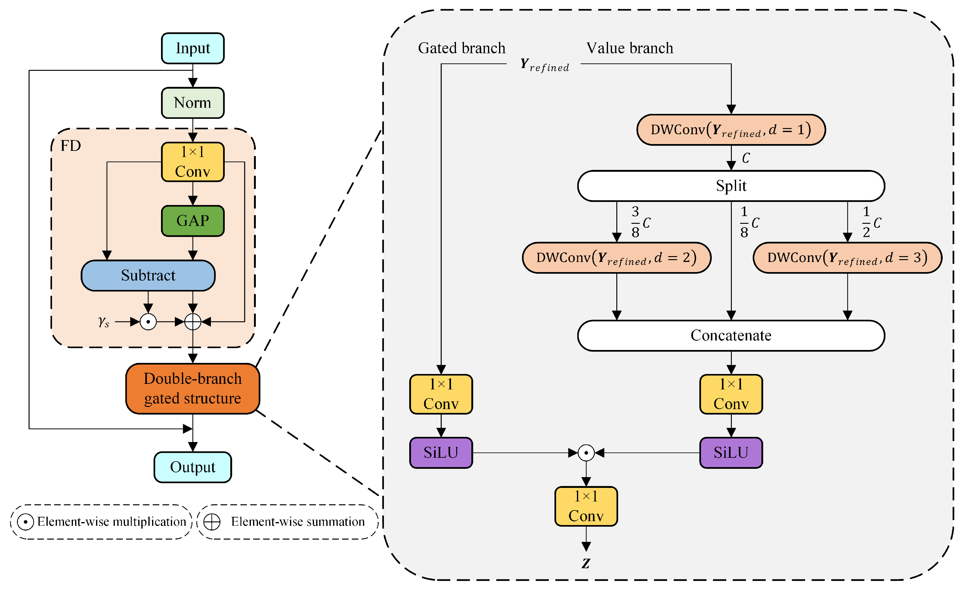
The Dual-Gated Fusion (DGF) module is the core component of SCGHN. DGF is composed of a Feature Decomposition (FD) unit, a dual-branch gating structure, and a gated fusion mechanism. It achieves dynamic feature selection and fusion through multi-stage gated aggregation. By integrating feature decomposition with adaptive gating strategies, this module effectively suppresses redundant information while enhancing feature representation. The detailed framework of DGF is shown in Figure 3.

The core objective of the Feature Decomposition (FD) unit is to separate global and local information while enhancing the representational capacity of local features. Firstly, FD employs a 1 × 1 convolutional layer for linear transformation of the input features, then employs global average pooling to extract global information, and finally enhances local features through a learnable scaling factor ${\gamma }_s$.

The input features $X\in {\mathbb{R}}^{B\times C\times H\times W}$ are given, where B denotes the batch size, C denotes the number of channels, H and W correspond to the feature map’s height and width. A linear transformation is first applied to the input features via a 1 × 1 convolutional layer. The mathematical formulation is shown in Equation (16):

$$Y={\mathrm{Conv}}_{1\times 1}\left(X\right)=W_{1\times 1}\ast X+b_{1\times 1}$$

(16)

where ${\mathrm{Conv}}_{1\times 1}$ denotes the 1 × 1 convolution operation, $W\in {\mathbb{R}}^{C_{out}\times C\times 1\times 1}$ is the convolutional kernel weights, $b_{1\times 1}\in {\mathbb{R}}^{C_{out}}$ is the bias term, and $C_{out}$ is the number of output channels. In this module, $C_{out}$ is typically set equal to C. The symbol “ * ” denotes the convolution operation.

After applying the linear transformation to the input features, the global average pooling operation is employed to extract global contextual information, as shown in Equation (17):

$$Y_{global}=GAP\left(Y\right)={\displaystyle \frac{1}{H\times W}}\sum _{i=1}^H\sum _{j=1}^W{Y}_{:,:,i,j}$$

(17)

where $Y_{global}$ is the global feature, which is obtained by computing the average value over all spatial locations for each channel, and its shape is ${\mathbb{R}}^{B\times C\times 1\times 1}$.

After extracting the global features, a learnable scaling factor ${\gamma }_s$ is utilized to enhance the local features. First, the local features are computed as shown in Equation (18):

$$Y_{local}=Y-Y_{global}$$

(18)

Subsequently, the local features are adaptively adjusted through element-wise multiplication and the scaling factor, as shown in Equation (19):

$$Y_{refined}=Y+{\gamma }_s\odot Y_{local}$$

(19)

where ${\gamma }_s$ is a learnable scaling factor initialized to 0, $Y_{local}$ is the local feature, $Y_{global}$ is the global feature, $Y_{refined}$ is the refined feature, and ⊙ denotes element-wise multiplication. This operation enables the model to adaptively improve the representational capacity of local features.

The dual-branch gating structure consists of a gated branch and a value branch, which are designed to generate gating signals and extract multi-scale features. Ultimately, the features are enhanced and redundancies suppressed through gated weighted fusion, thereby improving the model’s discriminative capability for complex land-cover objects.

In the gated branch, the refined feature $Y_{refined}$ is first processed by a 1 × 1 convolution, followed by the SiLU activation function to generate the gating signal, as shown in Equation (20):

$$G_{pre}={\mathrm{Conv}}_{1\times 1}\left(Y_{refined}\right)=W_g\ast Y_{refined}+b_g$$

(20)

where $W_g\in {\mathbb{R}}^{C\times C\times 1\times 1}$ is the weights of the 1 × 1 convolution in the gated branch, and $b_g\in {\mathbb{R}}^C$ is the bias term.

The SiLU activation function is defined in Equation (21):

$$SiLU\left(x\right)=x·Sigmoid\left(x\right)={\displaystyle \frac{x}{1+e^{-x}}}$$

(21)

Consequently, the gating signal G is as shown in Equation (22):

$$G=SiLU\left(G_{pre}\right)$$

(22)

The 1 × 1 convolution reduces channel dimensionality, thereby decreasing computational complexity. Meanwhile, compared to ReLU, the SiLU introduces a smooth gating mechanism, enhancing the nonlinear representation capabilities for subtle spectral features while preserving positive excitation and gradient stability.

The value branch extracts multi-scale features through a multi-stage dilated convolution. The multi-stage dilated convolution consists of three depth-wise separable convolutions with different dilation rates, where the dilation rates d is configured to 1, 2 and 3.

A depth-wise separable convolution can be resolved into a depth-wise convolution and a point-wise convolution. For an input feature $X_{in}\in {\mathbb{R}}^{B\times C\times H\times W}$ (where $X_{in}$ corresponds to the adjusted refined feature $Y_{refined}$), the formulation of the depth-wise convolution is given in Equation (23):

$$X_{dw}=DWConv\left(X_{in}\right)=\sum _{k=1}^K{W}_{dw,k}\ast X_{in,k}$$

(23)

where $W_{dw,k}\in {\mathbb{R}}^{1\times k\times k}$ denotes the depth-wise convolution kernel for the k-th channel, which operates on the k-th channel of the input feature. The point-wise convolution is a 1 × 1 convolution for channel dimension adjustment.

In the multi-stage dilated convolution, depth-wise separable convolutions with different dilation rates are computed separately, as shown in Equations (24)–(26):

$$V_l=DWConv\left(Y_{refined},d=1\right)$$

(24)

$$V_m=DWConv\left(Y_{refined},d=2\right)$$

(25)

$$V_h=DWConv\left(Y_{refined},d=3\right)$$

(26)

where $V_l$ is the low-level feature, $V_m$ is the medium-level feature, and $V_h$ is the high-level feature. First, the channel dimension C of $V_l$ is split according to the ratio (1:3:4). After that, $V_l$ retains ${\displaystyle \frac{1}{8}}C$, while ${\displaystyle \frac{3}{8}}C$ and ${\displaystyle \frac{1}{2}}C$ are allocated to $V_m$ and $V_h$.

Subsequently, these features are concatenated along the channel dimension, using a 1 × 1 convolution operation on the concatenated features. Finally, the multi-scale feature V is generated through the SiLU activation function, as shown in Equation (27):

$$V=SiLU\left({\mathrm{Conv}}_{1\times 1}\left(Concat\left(V_l,V_m,V_h\right)\right)\right)$$

(27)

The gated fusion mechanism processes the outputs of the gated branch and value branch through the SiLU activation function. Subsequently, the processed results undergo element-wise multiplication to achieve dynamic feature selection.

First, the SiLU function is used to obtain the gating signal G and the value branch output V, as shown in Equations (28) and (29):

$$G^{\prime }=SiLU\left(G\right)$$

(28)

$$V^{\prime }=SiLU\left(V\right)$$

(29)

After that the element-wise multiplication is performed to obtain the fused feature Z, as shown in Equation (30):

$$Z=G^{\prime }\odot V^{\prime }$$

(30)

where ⊙ denotes element-wise multiplication.

Finally, the fused feature Z is input into the Lightweight Classification Decision module to obtain the classification probability. This gated fusion mechanism dynamically selects features through the SiLU function and element-wise multiplication, enabling this model to concentrate on significant feature channels while mitigating the influence of redundant information. Consequently, the model achieves enhanced performance and efficiency in tasks of HSIC.

3. Experimental Results and Analysis

The structure of this section is as follows. Section 3.1 elaborates three hyperspectral datasets for evaluating the SCGHN model. Section 3.2 presents the experimental setup. Section 3.3 analyzes the impact of key parameter settings on the SCGHN model’s performance. Section 3.4 validates the contributions of the core modules (SCPC module and DGF module) through ablation experiments. Section 3.5 compares the classification performance of the proposed SCGHN model with state-of-the-art networks and visualizes the spatial distribution characteristics of the results. Section 3.6 evaluates the complexity of the SCGHN model, highlighting its lightweight advantages through comparisons with other models.

3.1. Hyperspectral Datasets

In our experiments, three hyperspectral datasets are utilized to evaluate the performance of the proposed SCGHN model.

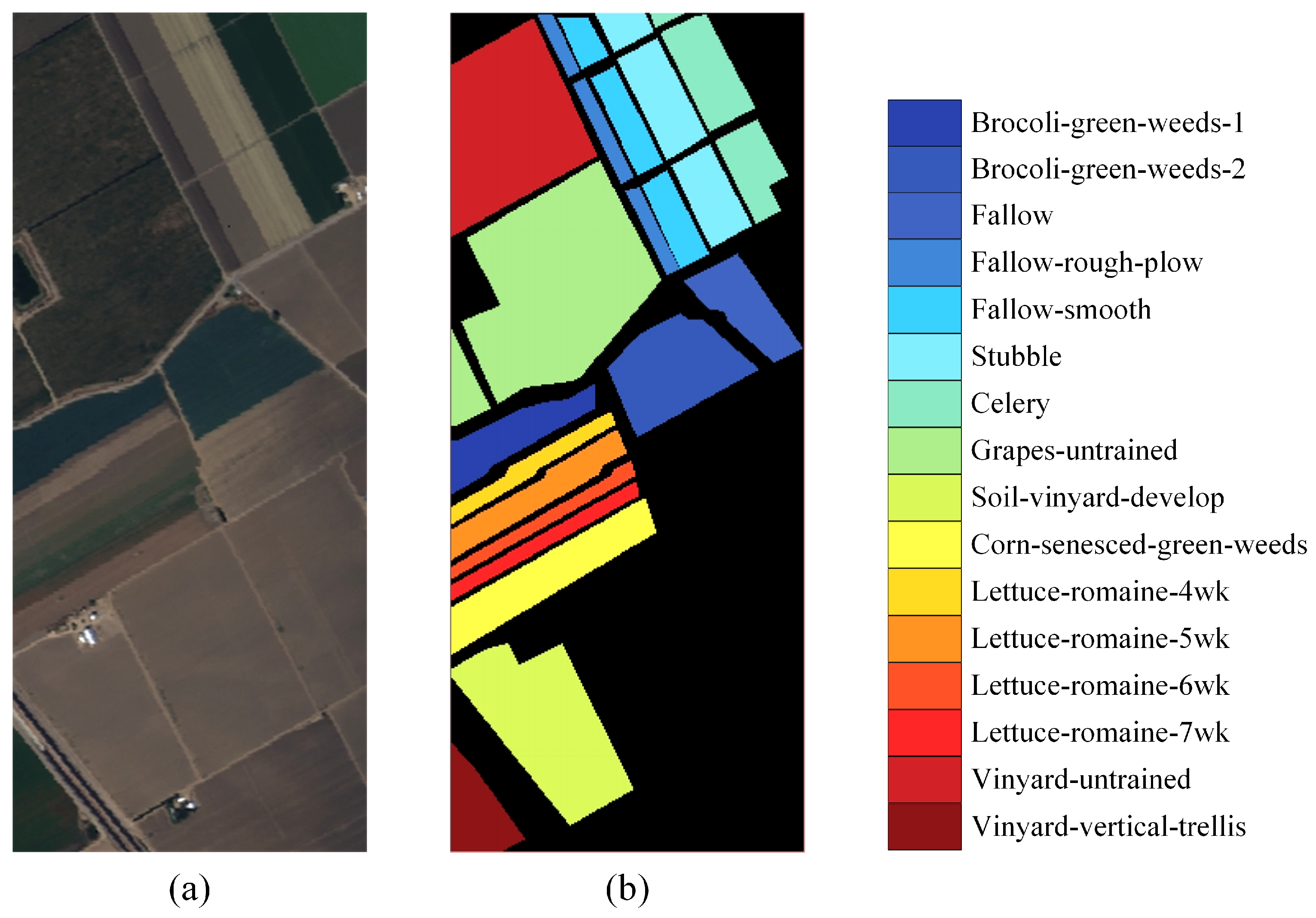
(1) Salinas: The Salinas dataset [38] is acquired by the AVIRIS imaging spectrometer over Salinas Valley, CA, USA, with a spatial resolution of 3.7 m and covering a 512 × 217-pixel area. The raw data contain 224 spectral bands, with 204 effective bands retained after discarding 20 water-absorption bands. Figure 4 displays the false-color map and its corresponding ground-truth map. This dataset contains 16 crop categories with a total of 54,129 labeled samples. Since SCGHN is a lightweight model and because of the high intra-class spectral similarity inherent in the Salinas dataset, a training ratio of 0.5% is sufficient to capture the typical spectral features of each crop category, while the 99% test set allows for a more rigorous evaluation of the model’s generalization capability to subtle intra-class variations. In summary, this dataset is split into 0.5% as the training set, 0.5% as the validation set, and 99% as the testing set, as detailed in

Table 1. Training, validation and test sample numbers in the Salinas dataset.

Class NO.	Land Cover Type	Train Num	Valid Num	Test Num
C1	Brocoli-green-weeds-1	10	10	1989
C2	Brocoli-green-weeds-2	18	19	3689
C3	Fallow	10	10	1956
C4	Fallow-rough-plow	7	7	1380
C5	Fallow-smooth	13	14	2651
C6	Stubble	19	20	3920
C7	Celery	18	18	3543
C8	Grapes-untrained	56	57	11,158
C9	Soil-vinyard-develop	31	31	6141
C10	Corn-senesced-green-weeds	16	17	3245
C11	Lettuce-romaine-4wk	6	5	1057
C12	Lettuce-romaine-5wk	10	9	1908
C13	Lettuce-romaine-6wk	5	4	907
C14	Lettuce-romaine-7wk	6	5	1059
C15	Vinyard-untrained	36	36	7196
C16	Vinyard-vertical-trellis	9	9	1789
	Total	270	271	53,588

.

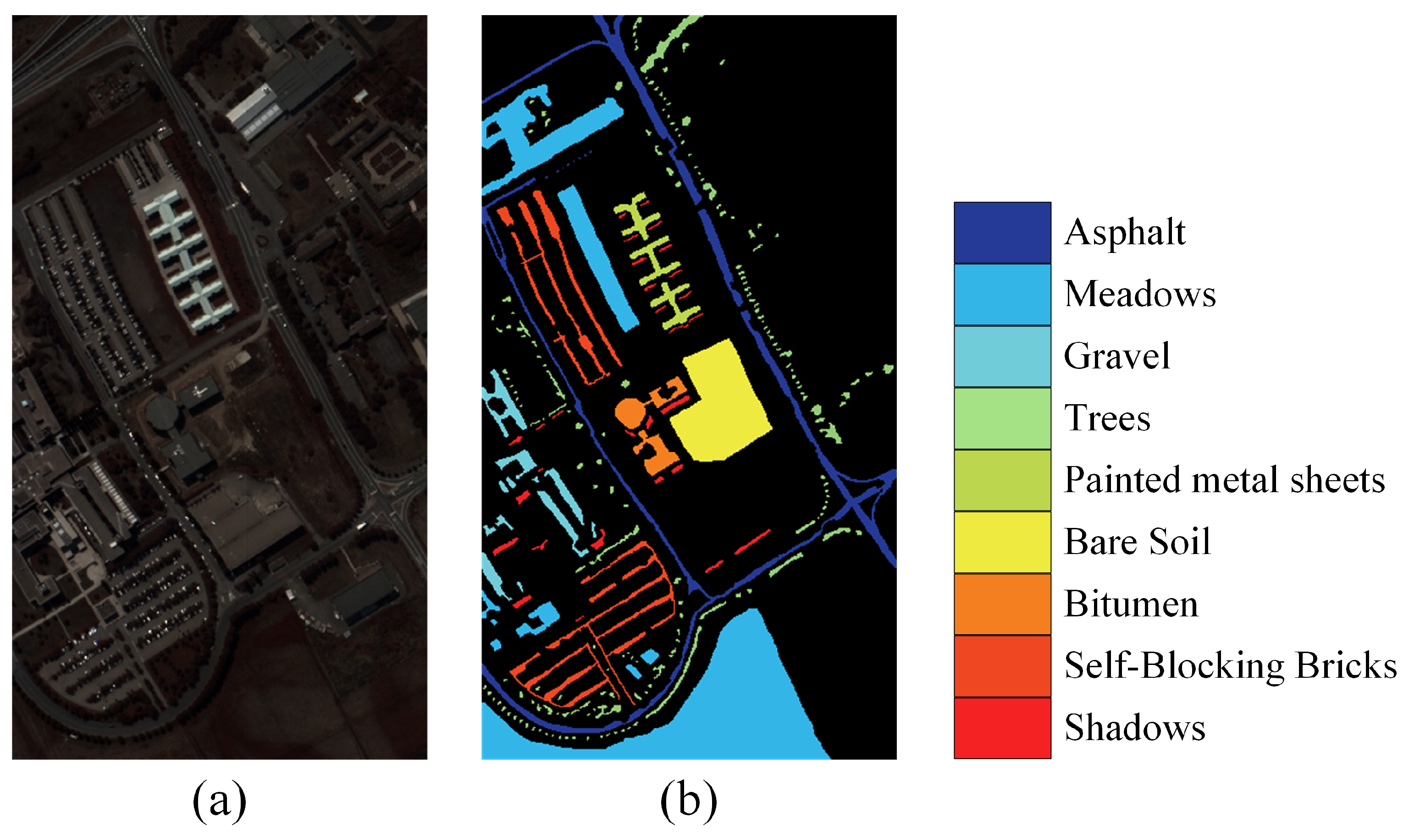
(2) Pavia University: The Pavia University dataset [38] is a hyperspectral remote sensing dataset acquired by the German ROSIS-03 imaging spectrometer in Pavia, Italy, in 2003 for urban land-cover classification and analysis. The raw data contain 115 spectral bands (0.43–0.86 $\mathsf{\mu }$m), with 103 effective bands retained after removing 12 noise-corrupted bands. They exhibit a 1.3 m spatial resolution and dimensions of 610 × 340 pixels. The dataset comprises 42,776 labeled samples categorized into nine urban land-cover types, including asphalt, meadows, trees, metal sheets, bare soil and bricks. Figure 5 illustrates the false-color map and its corresponding ground-truth map. Due to the low parameter count of SCGHN and the significant inter-class spectral confusion in the Pavia University dataset, a training ratio of 1% provides sufficient information for the model to learn key distinctions between categories, while the high 98% test ratio allows for more rigorous verification of the model’s generalization capability in complex urban scenarios. In summary, this dataset is split into 1% as the training set, 1% as the validation set, and 98% as the testing set, as detailed in

Table 2. Training, validation and test sample numbers in the Pavia University dataset.

Class NO.	Land Cover Type	Train Num	Valid Num	Test Num
C1	Asphalt	66	66	6499
C2	Meadows	186	187	18,276
C3	Gravel	21	21	2057
C4	Trees	30	31	3003
C5	Painted metal sheets	13	14	1318
C6	Bare Soil	50	50	4929
C7	Bitumen	14	13	1303
C8	Self-Blocking Bricks	37	37	3608
C9	Shadows	10	9	928
	Total	427	428	41,921

.

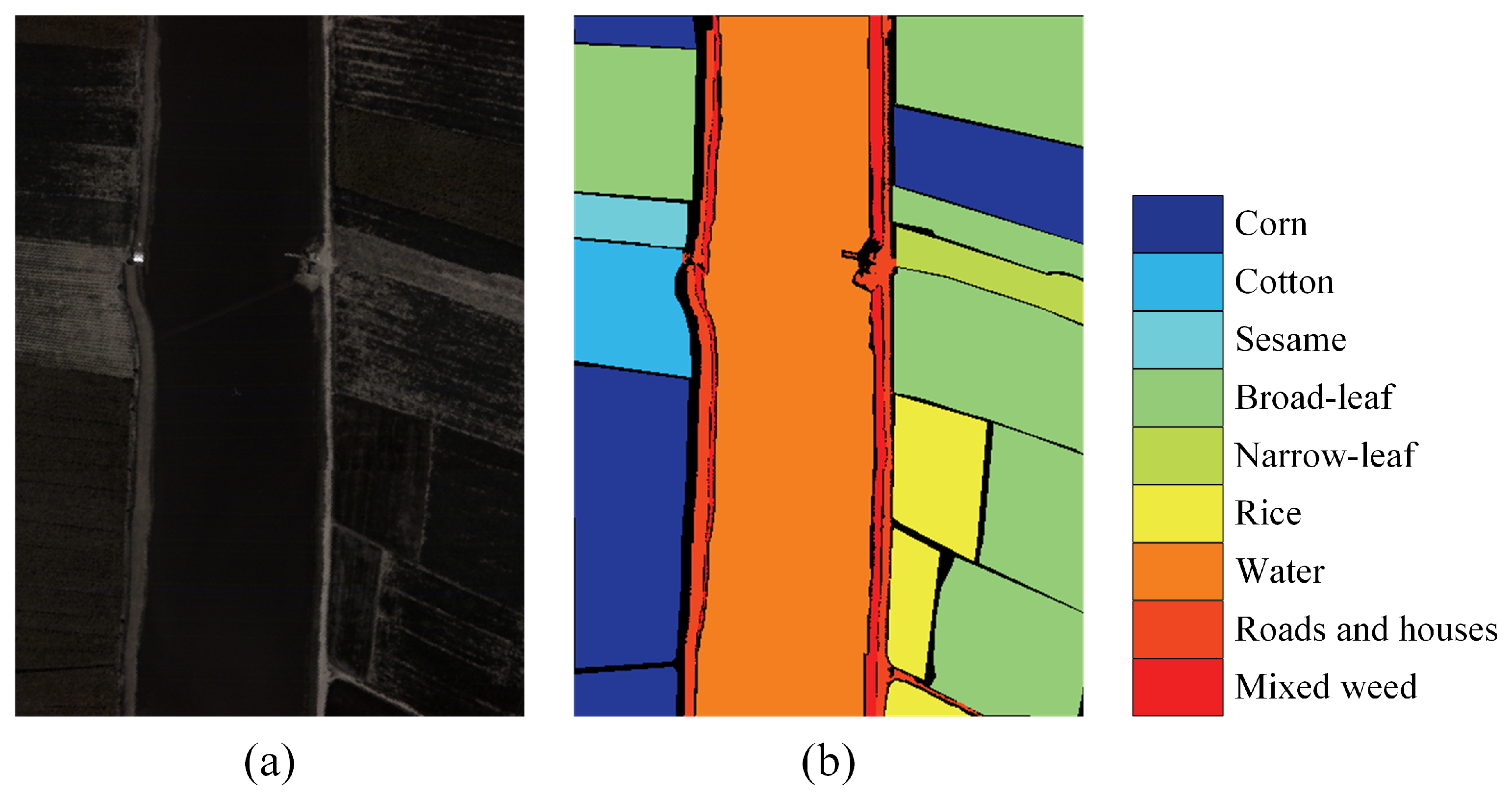
(3) WHU-Hi-LongKou: The WHU-Hi-LongKou dataset [39] was developed by Wuhan University in collaboration with international research teams. It was acquired through a UAV-mounted Hyperion hyperspectral sensor in Longkou City, Shandong Province, China, with a 0.46 m spatial resolution and covering a 500 × 500 pixels area. The dataset retains all original 270 spectral bands spanning the visible to near-infrared range (0.4–2.5 $\mathsf{\mu }$m). It contains 204,542 labeled samples categorized into nine complex land-cover classes. Figure 6 illustrates the false-color map and its corresponding ground-truth map. Due to the simple feature extraction process of SCGHN and the highly imbalanced class distribution of the WHU-Hi-LongKou dataset, a training ratio of 0.2% is sufficient to meet the learning requirements, while a testing ratio of 99.6% can adequately validate the model’s classification consistency under large-scale, class-imbalanced conditions. In summary, this dataset is split into 0.2% as the training set, 0.2% as the validation set, and 99.6% as the testing set, as detailed in

Table 3. Training, validation and test sample numbers in the WHU-Hi-LongKou dataset.

Class NO.	Land Cover Type	Train Num	Valid Num	Test Num
C1	Corn	69	69	34,373
C2	Cotton	17	16	8341
C3	Sesame	6	6	3019
C4	Broad-leaf	127	126	62,959
C5	Narrow-leaf	8	9	4134
C6	Rice	24	23	11,807
C7	Water	134	134	66,788
C8	Roads and houses	14	15	7095
C9	Mixed weed	10	11	5208
	Total	409	409	203,724

.

3.2. Experimental Setup

(1) Configurations: To ensure fair comparison, both the proposed method and all compared methods in this study were implemented using a deep learning framework of PyTorch 1.13.1.All experiments (training and testing) were conducted on a computational platform with a 13th Gen Intel CPU and an NVIDIA GeForce RTX 4060 GPU. The proposed method utilizes the Adam optimizer for parameter updates. The training configuration employs a learning rate of $1\times {10}^{-3}$, a batch size of 64, and runs for 100 epochs. For all compared methods, their configurations strictly followed the settings in their original papers to ensure their optimal performance, thereby guaranteeing the scientific validity and reliability of the comparative results.

(2) Evaluation Indicators: The classification performance of all approaches was evaluated using three standard metrics [40]: Overall Accuracy (OA), Average Accuracy (AA), and the Kappa coefficient ($\kappa$). OA reflects the total correctness of classification by computing the proportion of the number of correctly classified samples across all samples to the total number of samples. AA indicates the average per-class accuracy; it reflects the model’s balanced performance across each land-cover category. $\kappa$ chiefly reflects the agreement between the model’s classification outcomes and the ground-truth labels. Higher values in these three metrics correspond to superior performance in the classification task. The formulas for calculating OA, AA and $\kappa$ [41] are given by Equations (31)–(33):

$$OA={\displaystyle \frac{{\sum }_{i=1}^C{x}_{ii}}{{\sum }_{i=1}^C{\sum }_{j=1}^C{x}_{ij}}}$$

(31)

$$AA={\displaystyle \frac{1}{C}}\sum _{i=1}^C\left({\displaystyle \frac{x_{ii}}{{\sum }_{j=1}^C{x}_{ij}}}\right)$$

(32)

$$\kappa ={\displaystyle \frac{P_o-P_e}{1-P_e}}$$

(33)

where C is the total number of land cover classes, $x_{ii}$ is the number of correctly classified samples for the i-th class, and the denominator represents the total number of labeled samples. $\left({\displaystyle \frac{x_{ii}}{{\sum }_{j=1}^C{x}_{ij}}}\right)$ is the individual classification accuracy for the i-th class. $P_o$ is the overall accuracy, and $P_e$ ($P_e={\displaystyle \frac{1}{N^2}}{\sum }_{i=1}^C\left({\sum }_{j=1}^C{x}_{ij}\times {\sum }_{j=1}^C{x}_{ji}\right)$, where N is the total number of samples) is the expected random agreement rate.

3.3. Analysis on the Settings of Key Parameters

In this parameter analysis, we analyse the influence of critical hyperparameters on the method’s classification accuracy, including the patch size of input cubes, batch size and learning rate.

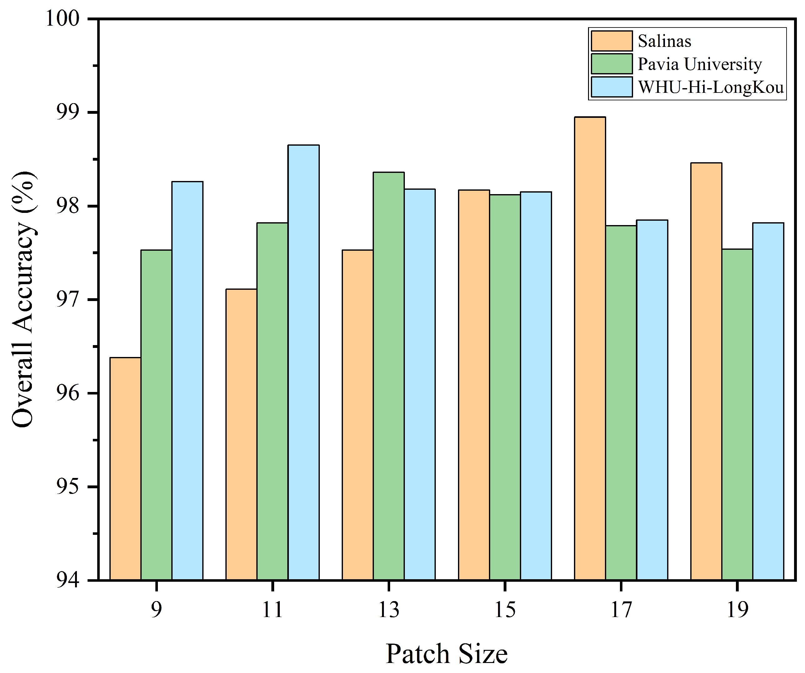
(1) Patch Size: To research the impact of patch size on classification performance, all candidate values should be set to odd numbers to ensure the central pixel is aligned with the target ground object. A smaller patch size facilitates capturing local fine spectral-spatial features, a larger patch size helps integrate broader contextual information, and an excessively large patch size needs to be avoided to prevent a sharp increase in the computational load of the lightweight model. Therefore, we selected candidate values of 9, 11, 13, 15, 17 and 19 for patch size while keeping other parameters unchanged. Figure 7 shows the OA of the model under different patch sizes across three datasets. As clearly demonstrated, the OA of the Salinas dataset increases with larger patch sizes and reaches its optimal value at 17. For the Pavia University dataset, the optimal classification accuracy was observed at the patch size of 13. For the WHU-Hi-LongKou dataset, the OA attains its highest value at a patch size of 11. Through a comprehensive consideration of the distinctions among different datasets in spatial resolution, complexity of land-cover types, and spectral discrepancies, while incorporating the experimental data presented in Figure 7, we set the patch size to 17 for Salinas, 13 for Pavia University, and 11 for WHU-Hi-LongKou to optimize classification effectiveness across diverse datasets.

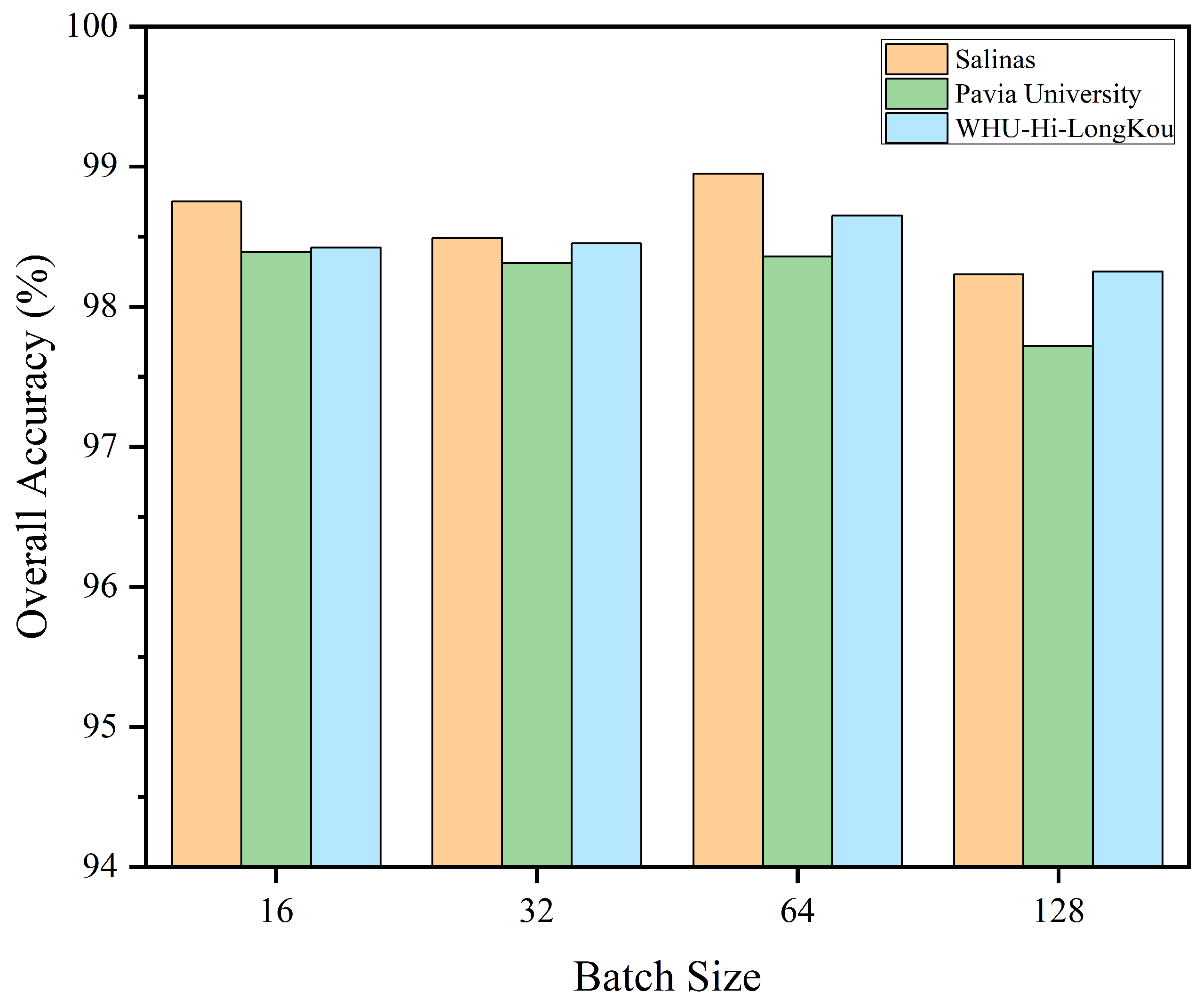
(2) Batch Size: The establishment of batch size is critical to a model’s classification accuracy. We select candidate values of 16, 32, 64 and 128 for batch size. As illustrated in Figure 8, the Salinas dataset achieves the highest OA at a batch size of 64. The Pavia University dataset performs best when the batch size is 16, but its accuracy difference from the batch size of 64 is marginal. For the WHU-Hi-LongKou dataset, the OA attains its highest value at a batch size of 64. Therefore, we set the batch size to 64 for all datasets.

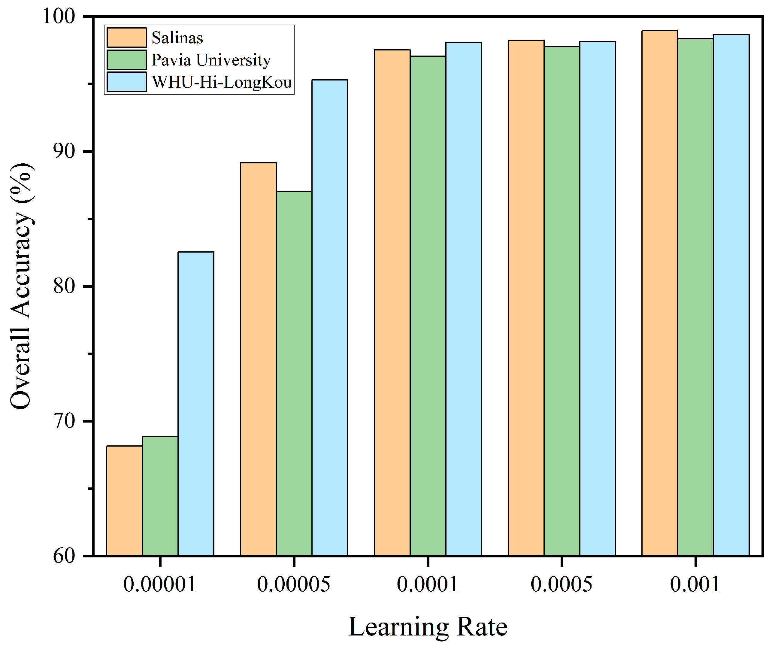
(3) Learning Rate: The learning rate plays a critical role in model training, exerting a substantial influence on the optimization process and performance. We selected candidate values of $1\times {10}^{-5}$, $5\times {10}^{-5}$, $1\times {10}^{-4}$, $5\times {10}^{-4}$ and $1\times {10}^{-3}$ to research its impact. Figure 9 displays the variations in OA for the three datasets across diverse learning rates. Obviously, when the learning rate increases from $1\times {10}^{-5}$, the OA of the Salinas, Pavia University and WHU-Hi-LongKou datasets initially rises significantly, indicating that higher learning rates facilitate better model convergence and optimization within a certain range. When the learning rate reaches $1\times {10}^{-4}$, the OA of all datasets stabilizes at a high level and remains relatively consistent. The OA peaks at a learning rate of $1\times {10}^{-3}$ across all datasets. Therefore, we set the learning rate to $1\times {10}^{-3}$ to balance training efficiency and classification performance.

3.4. Ablation Experiments

To sufficiently prove the effectiveness of the proposed model, ablation experiments on the core components of SCGHN (SCPC module and DGF module) were conducted across all three datasets. Four combinations were systematically evaluated, and the influence of each component on the model was analyzed in terms of classification accuracy. Specifically: The first combination (3D-2D Hybrid Convolution, hereafter dubbed HC32) includes only 3D convolutional layers, 2D convolutional layers, and a lightweight classification decision block. This combination is the reference model; The second combination (HC32 + SCPC) replaces the 2D convolutional layers in HC32 with the SCPC module; The third combination (HC32+DGF) introduces the DGF module into HC32; The fourth combination (SCGHN) integrates the DGF module into (HC32 + SCPC) to form the complete proposed model. The experimental results are shown in

Table 4. Ablation experiments of the proposed model on three datasets, with comparisons of OA (%), AA (%) and $\kappa$ × 100 (best results are bolded).

	Group Nums	Methods	OA (%)	AA(%)	$\mathit{\kappa }\times 100$
Salinas	1	HC32	$92.76\pm 0.39$	$88.47\pm 0.22$	$91.91\pm 0.43$
	2	HC32 + SCPC	$96.23\pm 0.31$	$95.74\pm 0.68$	$95.80\pm 0.36$
	3	HC32 + DGF	$96.14\pm 0.21$	$95.16\pm 0.54$	$95.69\pm 0.29$
	4	SCGHN	$\mathbf{98}.\mathbf{95}\pm \mathbf{0}.\mathbf{15}$	$\mathbf{98}.\mathbf{62}\pm \mathbf{0}.\mathbf{33}$	$\mathbf{98}.\mathbf{83}\pm \mathbf{0}.\mathbf{17}$
Pavia University	1	HC32	$94.48\pm 0.12$	$90.19\pm 0.15$	$92.61\pm 0.16$
	2	HC32 + SCPC	$95.98\pm 0.49$	$92.98\pm 0.97$	$94.66\pm 0.65$
	3	HC32 + DGF	$95.60\pm 0.23$	$92.96\pm 0.45$	$94.16\pm 0.31$
	4	SCGHN	$\mathbf{98}.\mathbf{36}\pm \mathbf{0}.\mathbf{10}$	$\mathbf{97}.\mathbf{17}\pm \mathbf{0}.\mathbf{14}$	$\mathbf{97}.\mathbf{82}\pm \mathbf{0}.\mathbf{13}$
WHU-Hi-LongKou	1	HC32	$97.09\pm 0.43$	$90.48\pm 1.61$	$96.17\pm 0.57$
	2	HC32 + SCPC	$97.62\pm 0.29$	$92.87\pm 0.55$	$96.86\pm 0.39$
	3	HC32 + DGF	$97.24\pm 0.47$	$92.81\pm 0.86$	$96.38\pm 0.61$
	4	SCGHN	$\mathbf{98}.\mathbf{65}\pm \mathbf{0}.\mathbf{39}$	$\mathbf{96}.\mathbf{88}\pm \mathbf{0}.\mathbf{17}$	$\mathbf{98}.\mathbf{23}\pm \mathbf{0}.\mathbf{51}$

,

Table 5. Ablation experiments of the proposed model on three datasets, with comparisons of parameters and flops (best results are bolded).

	Group Nums	Methods	Parameters/K	FLOPs/M
Salinas	1	HC32	130.48	23.42
	2	HC32+SCPC	34.36	7.09
	3	HC32+DGF	151.01	26.83
	4	SCGHN	54.88	10.50
Pavia University	1	HC32	130.03	11.32
	2	HC32+SCPC	33.91	3.49
	3	HC32+DGF	150.56	12.95
	4	SCGHN	54.44	5.12
WHU-Hi-LongKou	1	HC32	130.12	6.90
	2	HC32+SCPC	34.09	2.17
	3	HC32+DGF	150.78	7.89
	4	SCGHN	54.51	3.15

and

Table 6. Ablation experiments of the proposed model on three datasets, with comparisons of training time and testing time (best results are bolded).

	Group Nums	Methods	Train (s)	Test (s)
Salinas	1	HC32	5.67	3.38
	2	HC32+SCPC	7.32	4.09
	3	HC32+DGF	19.20	8.08
	4	SCGHN	8.34	4.59
Pavia University	1	HC32	7.36	4.41
	2	HC32+SCPC	8.30	5.17
	3	HC32+DGF	9.59	5.82
	4	SCGHN	13.85	9.68
WHU-Hi-LongKou	1	HC32	6.01	2.69
	2	HC32+SCPC	7.24	4.13
	3	HC32+DGF	8.94	4.69
	4	SCGHN	10.84	6.54

.

To comprehensively research the contributions of SCGHN components, the aforementioned ablation experiments were designed. The first combination (HC32) serves as the reference model, whose performance establishes the comparative benchmark. The second combination (HC32 + SCPC) replaces the 2D convolutional layers in HC32 with the SCPC module. Experimental results demonstrate that this configuration achieves significant performance improvements across all datasets compared to HC32, while reducing parameters and FLOPs by approximately 73.7% and 69.8%. This indicates that the SCPC module not only effectively reduces model complexity but also enhances feature extraction efficiency, thereby improving classification accuracy with a lightweight architecture. The third combination (HC32 + DGF) introduces the DGF module into HC32, which increases both parameters and FLOPs, but yields substantial performance gains over HC32. This suggests that the DGF module positively contributes to feature fusion and optimizes the feature processing pipeline despite added computational costs. The fourth combination integrates the DGF module into (HC32 + SCPC) to form the complete SCGHN model. As shown in Table 4 and Table 5, SCGHN achieves the highest classification metrics (OA, AA, $\kappa$) on all datasets while maintaining reasonable parameter and FLOPs budgets. Taking the Salinas dataset as an example, SCGHN requires only 54.88 K parameters and 10.5 M FLOPs, representing reductions of approximately 63.6% and 61.0%, respectively, compared to (HC32 + DGF), which confirms that the synergistic interaction of components in SCGHN achieves a more efficient architecture while avoiding excessive computational burdens.

Table 6 presents the training and testing time costs in the ablation experiments. The first combination (HC32) requires the shortest computation time, whereas SCGHN consumes the longest computation time. This is attributed to two factors. Firstly, the SCPC module introduces additional computational steps during feature extraction despite its structural simplification. Secondly, the DGF module increases the complexity of feature fusion. The classification metrics in Table 4, Table 5 and Table 6 collectively demonstrate that SCGHN achieves an optimal balance among model parameters, computational costs, inference time and classification accuracy.

In conclusion, the experimental analysis clearly reveals the contributions of both the SCPC module and DGF module to performance enhancement, while confirming the superiority of SCGHN in hyperspectral classification tasks. These results provide robust evidence for the practical effectiveness of the proposed model.

3.5. Comparison with State-of-the-Art Methods

To further highlight the advantages of our proposed SCGHN, several representative methods were selected for comparative experiments, including 2DCNN [26], 3DCNN [42], SPRN [43], SpectralFormer [44], CAEVT [45], GAHT [46], SSFTT [33], GSC-ViT [34], and ${\mathrm{S}}^2$Mamba [47].

Table 7. Classification performance of different models in the Salinas dataset (best results are bolded).

Class	2DCNN	3DCNN	SPRN	SpectralFormer	CAEVT	GAHT	SSFTT	GSC-ViT	${\mathbf{S}}^2$Mamba	SCGHN
1	$12.97\pm 30.33$	$88.19\pm 20.41$	$99.83\pm 0.31$	$94.08\pm 1.95$	$98.52\pm 2.39$	$98.76\pm 3.45$	$99.89\pm 0.16$	$99.42\pm 0.90$	$99.39\pm 0.92$	$\mathbf{100}.\mathbf{00}\pm \mathbf{0}.\mathbf{00}$
2	$76.77\pm 38.87$	$99.09\pm 1.19$	$\mathbf{100}.\mathbf{00}\pm \mathbf{0}.\mathbf{00}$	$98.89\pm 0.54$	$99.74\pm 0.20$	$99.66\pm 0.50$	$99.67\pm 0.33$	$99.42\pm 0.90$	$99.39\pm 1.26$	$99.96\pm 0.05$
3	$35.81\pm 34.86$	$61.03\pm 8.35$	$95.92\pm 3.82$	$86.89\pm 7.77$	$90.76\pm 7.96$	$95.19\pm 4.76$	$99.85\pm 0.44$	$89.29\pm 12.55$	$98.20\pm 2.11$	$\mathbf{99}.\mathbf{88}\pm \mathbf{0}.\mathbf{17}$
4	$\mathbf{99}.\mathbf{20}\pm \mathbf{1}.\mathbf{52}$	$95.19\pm 3.26$	$97.20\pm 1.78$	$92.07\pm 4.13$	$95.07\pm 3.92$	$97.99\pm 2.06$	$98.40\pm 1.52$	$98.14\pm 2.33$	$98.57\pm 1.91$	$95.77\pm 5.16$
5	$57.71\pm 38.63$	$92.75\pm 1.82$	$97.74\pm 2.14$	$84.21\pm 2.21$	$92.55\pm 4.91$	$96.96\pm 2.62$	$97.93\pm 2.03$	$93.65\pm 6.88$	$98.42\pm 1.93$	$\mathbf{99}.\mathbf{13}\pm \mathbf{0}.\mathbf{41}$
6	$97.86\pm 4.74$	$99.79\pm 0.18$	$100.00\pm 0.01$	$99.34\pm 0.78$	$99.57\pm 0.75$	$99.91\pm 0.28$	$99.74\pm 0.51$	$99.97\pm 0.06$	$99.65\pm 0.82$	$\mathbf{100}.\mathbf{00}\pm \mathbf{0}.\mathbf{00}$
7	$88.48\pm 3.51$	$99.61\pm 0.20$	$99.98\pm 0.03$	$98.46\pm 0.64$	$99.52\pm 0.71$	$\mathbf{99}.\mathbf{91}\pm \mathbf{0}.\mathbf{12}$	$99.72\pm 0.25$	$99.36\pm 1.45$	$99.83\pm 0.26$	$98.76\pm 0.82$
8	$92.18\pm 1.12$	$84.48\pm 7.39$	$92.73\pm 3.00$	$82.19\pm 1.95$	$87.29\pm 3.49$	$90.93\pm 3.22$	$96.55\pm 2.03$	$94.12\pm 3.83$	$95.76\pm 1.79$	$\mathbf{98}.\mathbf{66}\pm \mathbf{0}.\mathbf{25}$
9	$95.13\pm 3.45$	$98.60\pm 0.78$	$99.87\pm 0.17$	$95.55\pm 2.81$	$98.39\pm 1.82$	$99.49\pm 0.67$	$99.93\pm 0.12$	$99.40\pm 1.42$	$99.88\pm 0.12$	$\mathbf{99}.\mathbf{97}\pm \mathbf{0}.\mathbf{04}$
10	$66.78\pm 18.07$	$74.41\pm 3.24$	$93.76\pm 2.47$	$83.35\pm 4.98$	$91.40\pm 4.02$	$94.74\pm 1.53$	$96.73\pm 2.99$	$93.13\pm 5.73$	$\mathbf{98}.\mathbf{13}\pm \mathbf{2}.\mathbf{14}$	$97.71\pm 0.63$
11	$18.31\pm 15.02$	$15.81\pm 7.91$	$97.47\pm 2.77$	$83.47\pm 11.08$	$91.29\pm 7.78$	$95.44\pm 3.67$	$99.11\pm 2.02$	$91.81\pm 8.85$	$98.73\pm 1.10$	$\mathbf{100}.\mathbf{00}\pm \mathbf{0}.\mathbf{00}$
12	$62.41\pm 28.70$	$97.76\pm 5.66$	$\mathbf{99}.\mathbf{90}\pm \mathbf{0}.\mathbf{14}$	$98.45\pm 2.31$	$99.17\pm 1.83$	$99.70\pm 0.58$	$99.16\pm 1.13$	$98.11\pm 2.36$	$99.88\pm 0.19$	$99.41\pm 0.58$
13	$66.93\pm 24.58$	$83.78\pm 28.42$	$97.91\pm 2.13$	$90.04\pm 6.42$	$97.74\pm 3.55$	$95.95\pm 3.97$	$97.31\pm 4.02$	$96.96\pm 4.82$	$\mathbf{99}.\mathbf{84}\pm \mathbf{0}.\mathbf{47}$	$96.99\pm 1.85$
14	$51.42\pm 38.54$	$88.88\pm 13.60$	$98.37\pm 1.41$	$96.38\pm 2.97$	$98.56\pm 1.46$	$98.39\pm 1.21$	$93.28\pm 7.51$	$\mathbf{98}.\mathbf{96}\pm \mathbf{1}.\mathbf{73}$	$98.77\pm 1.06$	$94.37\pm 3.88$
15	$20.98\pm 12.44$	$42.74\pm 14.72$	$86.58\pm 4.55$	$74.87\pm 4.28$	$83.55\pm 4.45$	$82.83\pm 6.93$	$96.18\pm 2.02$	$87.77\pm 4.95$	$95.78\pm 1.59$	$\mathbf{98}.\mathbf{86}\pm \mathbf{1}.\mathbf{00}$
16	$40.67\pm 32.63$	$65.57\pm 9.30$	$96.92\pm 2.92$	$86.24\pm 4.71$	$94.86\pm 2.87$	$95.15\pm 2.97$	$98.35\pm 1.67$	$93.79\pm 9.33$	$97.53\pm 2.31$	$\mathbf{98}.\mathbf{38}\pm \mathbf{0}.\mathbf{16}$
OA (%)	$68.54\pm 5.79$	$81.54\pm 2.14$	$95.73\pm 0.55$	$88.41\pm 1.04$	$93.03\pm 1.05$	$94.61\pm 0.80$	$98.07\pm 0.59$	$95.31\pm 1.01$	$98.04\pm 0.33$	$\mathbf{98}.\mathbf{95}\pm \mathbf{0}.\mathbf{15}$
AA (%)	$61.47\pm 10.03$	$80.48\pm 4.26$	$97.14\pm 0.51$	$90.28\pm 1.56$	$94.87\pm 1.05$	$96.31\pm 1.14$	$98.24\pm 0.58$	$95.86\pm 1.06$	$98.59\pm 0.23$	$\mathbf{98}.\mathbf{62}\pm \mathbf{0}.\mathbf{33}$
$\kappa \times 100$	$64.43\pm 6.73$	$79.27\pm 2.46$	$95.24\pm 0.61$	$87.10\pm 1.16$	$92.24\pm 1.17$	$93.99\pm 0.90$	$97.85\pm 0.66$	$94.78\pm 1.13$	$98.31\pm 0.37$	$\mathbf{98}.\mathbf{83}\pm \mathbf{0}.\mathbf{17}$

,

Table 8. Classification performance of different models in the Pavia University dataset (best results are bolded).

Class	2DCNN	3DCNN	SPRN	SpectralFormer	CAEVT	GAHT	SSFTT	GSC-ViT	${\mathbf{S}}^2$Mamba	SCGHN
1	$91.81\pm 3.82$	$94.66\pm 1.10$	$97.94\pm 0.97$	$86.58\pm 2.24$	$98.01\pm 0.56$	$97.84\pm 0.89$	$98.12\pm 1.36$	$98.33\pm 0.59$	$96.45\pm 0.63$	$\mathbf{98}.\mathbf{93}\pm \mathbf{0}.\mathbf{48}$
2	$97.49\pm 1.26$	$97.16\pm 0.65$	$99.82\pm 0.17$	$97.74\pm 0.78$	$99.58\pm 0.19$	$99.49\pm 0.25$	$99.85\pm 0.19$	$99.40\pm 0.49$	$98.68\pm 0.23$	$\mathbf{99}.\mathbf{92}\pm \mathbf{0}.\mathbf{08}$
3	$63.74\pm 15.53$	$14.28\pm 4.49$	$91.15\pm 5.28$	$72.97\pm 3.41$	$85.68\pm 4.83$	$86.53\pm 4.47$	$91.37\pm 2.84$	$\mathbf{93}.\mathbf{38}\pm \mathbf{4}.\mathbf{47}$	$92.56\pm 3.49$	$89.30\pm 0.66$
4	$95.62\pm 2.09$	$82.27\pm 6.02$	$95.37\pm 1.71$	$91.45\pm 2.14$	$\mathbf{97}.\mathbf{13}\pm \mathbf{2}.\mathbf{01}$	$96.91\pm 0.74$	$94.78\pm 1.56$	$94.90\pm 1.54$	$96.02\pm 1.46$	$94.87\pm 0.85$
5	$98.55\pm 3.45$	$98.88\pm 1.15$	$99.98\pm 0.03$	$\mathbf{100}.\mathbf{00}\pm \mathbf{0}.\mathbf{00}$	$99.91\pm 0.15$	$\mathbf{100}.\mathbf{00}\pm \mathbf{0}.\mathbf{00}$	$99.92\pm 0.20$	$99.62\pm 0.55$	$99.58\pm 0.12$	$99.97\pm 0.04$
6	$91.14\pm 4.31$	$25.49\pm 2.20$	$98.36\pm 1.19$	$78.28\pm 2.11$	$98.42\pm 0.88$	$96.42\pm 1.86$	$98.97\pm 1.61$	$98.37\pm 2.14$	$98.40\pm 0.65$	$\mathbf{99}.\mathbf{05}\pm \mathbf{1}.\mathbf{22}$
7	$72.46\pm 5.95$	$7.04\pm 7.69$	$90.41\pm 4.88$	$61.07\pm 6.10$	$90.71\pm 4.89$	$87.78\pm 7.95$	$98.96\pm 0.91$	$92.62\pm 8.15$	$98.85\pm 0.86$	$\mathbf{99}.\mathbf{39}\pm \mathbf{0}.\mathbf{56}$
8	$85.46\pm 5.94$	$92.37\pm 1.93$	$92.99\pm 2.40$	$81.16\pm 3.88$	$95.19\pm 3.27$	$95.87\pm 2.65$	$93.41\pm 3.37$	$96.73\pm 1.89$	$\mathbf{98}.\mathbf{25}\pm \mathbf{0}.\mathbf{47}$	$95.85\pm 0.15$
9	$97.49\pm 3.63$	$99.17\pm 0.74$	$\mathbf{99}.\mathbf{43}\pm \mathbf{0}.\mathbf{35}$	$91.07\pm 4.16$	$99.02\pm 1.04$	$99.19\pm 0.79$	$90.83\pm 4.14$	$92.58\pm 2.89$	$97.08\pm 0.59$	$97.23\pm 1.37$
OA (%)	$92.29\pm 1.77$	$80.10\pm 0.77$	$97.73\pm 0.17$	$89.41\pm 0.54$	$97.69\pm 0.30$	$97.39\pm 0.37$	$97.92\pm 0.42$	$97.91\pm 0.43$	$98.06\pm 0.38$	$\mathbf{98}.\mathbf{36}\pm \mathbf{0}.\mathbf{10}$
AA (%)	$88.19\pm 2.22$	$67.93\pm 1.54$	$96.16\pm 0.71$	$84.48\pm 0.89$	$95.96\pm 0.65$	$95.56\pm 1.03$	$96.25\pm 0.63$	$96.21\pm 0.85$	$97.04\pm 0.49$	$\mathbf{97}.\mathbf{17}\pm \mathbf{0}.\mathbf{14}$
$\kappa \times 100$	$89.78\pm 2.33$	$72.42\pm 1.15$	$96.98\pm 0.23$	$85.86\pm 0.70$	$96.93\pm 0.39$	$96.53\pm 0.49$	$97.24\pm 0.56$	$97.23\pm 0.58$	$97.42\pm 0.51$	$\mathbf{97}.\mathbf{82}\pm \mathbf{0}.\mathbf{13}$

and

Table 9. Classification performance of different models in the WHU-Hi-LongKou dataset (best results are bolded).

Class	2DCNN	3DCNN	SPRN	SpectralFormer	CAEVT	GAHT	SSFTT	GSC-ViT	${\mathbf{S}}^2$Mamba	SCGHN
1	$96.46\pm 2.50$	$97.35\pm 0.91$	$\mathbf{99}.\mathbf{89}\pm \mathbf{0}.\mathbf{07}$	$99.32\pm 0.40$	$99.74\pm 0.17$	$99.72\pm 0.15$	$99.89\pm 0.08$	$99.56\pm 0.62$	$99.67\pm 0.17$	$99.84\pm 0.08$
2	$59.42\pm 41.21$	$73.70\pm 6.89$	$95.88\pm 1.58$	$88.20\pm 5.27$	$95.50\pm 2.89$	$96.96\pm 1.17$	$97.66\pm 2.40$	$97.87\pm 0.92$	$98.51\pm 0.89$	$\mathbf{99}.\mathbf{66}\pm \mathbf{0}.\mathbf{18}$
3	$0.00\pm 0.00$	$1.30\pm 1.79$	$88.82\pm 6.53$	$86.58\pm 4.27$	$88.49\pm 5.06$	$86.25\pm 11.02$	$92.41\pm 2.13$	$91.22\pm 4.83$	$94.26\pm 4.41$	$\mathbf{94}.\mathbf{57}\pm \mathbf{1}.\mathbf{32}$
4	$93.40\pm 3.23$	$96.39\pm 0.90$	$99.12\pm 0.48$	$96.71\pm 1.09$	$98.46\pm 0.65$	$98.66\pm 0.61$	$98.86\pm 0.33$	$99.01\pm 0.46$	$97.48\pm 0.17$	$\mathbf{99}.\mathbf{16}\pm \mathbf{0}.\mathbf{37}$
5	$4.04\pm 12.13$	$9.39\pm 10.00$	$90.08\pm 4.57$	$70.31\pm 9.89$	$91.21\pm 2.31$	$90.37\pm 3.61$	$91.75\pm 7.37$	$91.73\pm 3.04$	$92.46\pm 3.66$	$\mathbf{94}.\mathbf{48}\pm \mathbf{1}.\mathbf{19}$
6	$50.80\pm 32.77$	$94.74\pm 3.26$	$99.55\pm 0.48$	$95.15\pm 1.35$	$98.49\pm 1.21$	$99.08\pm 0.74$	$99.47\pm 0.27$	$97.84\pm 2.52$	$98.13\pm 1.25$	$\mathbf{99}.\mathbf{69}\pm \mathbf{0}.\mathbf{19}$
7	$99.87\pm 0.20$	$\mathbf{99}.\mathbf{99}\pm \mathbf{0}.\mathbf{01}$	$99.83\pm 0.13$	$99.91\pm 0.05$	$99.76\pm 0.38$	$99.72\pm 0.24$	$99.71\pm 0.17$	$99.57\pm 0.47$	$98.55\pm 0.35$	$98.69\pm 0.97$
8	$47.99\pm 34.31$	$77.86\pm 6.02$	$93.86\pm 2.99$	$82.71\pm 4.10$	$93.48\pm 1.58$	$90.80\pm 4.35$	$89.48\pm 3.28$	$89.94\pm 2.59$	$93.43\pm 2.08$	$\mathbf{95}.\mathbf{33}\pm \mathbf{1}.\mathbf{37}$
9	$41.48\pm 18.64$	$28.11\pm 9.59$	$89.72\pm 4.31$	$51.87\pm 12.23$	$90.16\pm 3.79$	$91.58\pm 3.00$	$85.39\pm 5.49$	$91.29\pm 4.31$	$\mathbf{93}.\mathbf{49}\pm \mathbf{3}.\mathbf{22}$	$90.48\pm 0.93$
OA (%)	$86.07\pm 3.10$	$91.14\pm 0.36$	$98.61\pm 0.18$	$95.44\pm 0.41$	$98.30\pm 0.28$	$98.33\pm 0.39$	$98.39\pm 0.15$	$98.39\pm 0.38$	$98.47\pm 0.17$	$\mathbf{98}.\mathbf{65}\pm \mathbf{0}.\mathbf{39}$
AA (%)	$54.83\pm 7.70$	$64.32\pm 1.33$	$95.19\pm 1.03$	$85.64\pm 2.45$	$95.03\pm 0.54$	$94.79\pm 1.66$	$94.96\pm 0.79$	$95.34\pm 0.96$	$96.16\pm 0.82$	$\mathbf{96}.\mathbf{88}\pm \mathbf{0}.\mathbf{17}$
$\kappa \times 100$	$81.43\pm 4.20$	$88.21\pm 0.47$	$98.17\pm 0.23$	$94.00\pm 0.54$	$97.77\pm 0.36$	$97.81\pm 0.52$	$97.88\pm 0.19$	$97.89\pm 0.50$	$98.09\pm 0.22$	$\mathbf{98}.\mathbf{23}\pm \mathbf{0}.\mathbf{50}$

record the OA, AA and $\kappa$ of each class for all compared models on the three HSI datasets (best results are bolded). Significantly, our proposed SCGHN achieves the optimal performance among all methods, with the highest OA, AA and $\kappa$.

Clearly, the SCGHN model demonstrates outstanding performance in the Salinas dataset. With only 0.5% training samples, its OA reaches 98.95 ± 0.15%, ranking first among all compared models and leading the second-best model by approximately 0.88%. It even achieves 100% classification accuracy in some categories. Although SCGHN does not achieve the best accuracy in partial categories, its overall OA is higher, reflecting SCGHN’s superior generalization capability. The AA and $\kappa$ values of SCGHN are 98.62 ± 0.33% and 98.83 ± 0.17%. For the Pavia University dataset, using only 1% training samples, SCGHN achieves an OA of 98.36 ± 0.10%, outperforming the second-best model by about 0.3%. In the WHU-Hi-LongKou dataset, with a training sample ratio of 0.2%, SCGHN still attains an OA of 98.65 ± 0.39%, surpassing the second-best model by approximately 0.04%. After 10 repeated experiments in each dataset, the OA, AA and $\kappa$ of SCGHN exhibit minimal fluctuations, demonstrating its high stability and reliable classification performance across the three datasets.

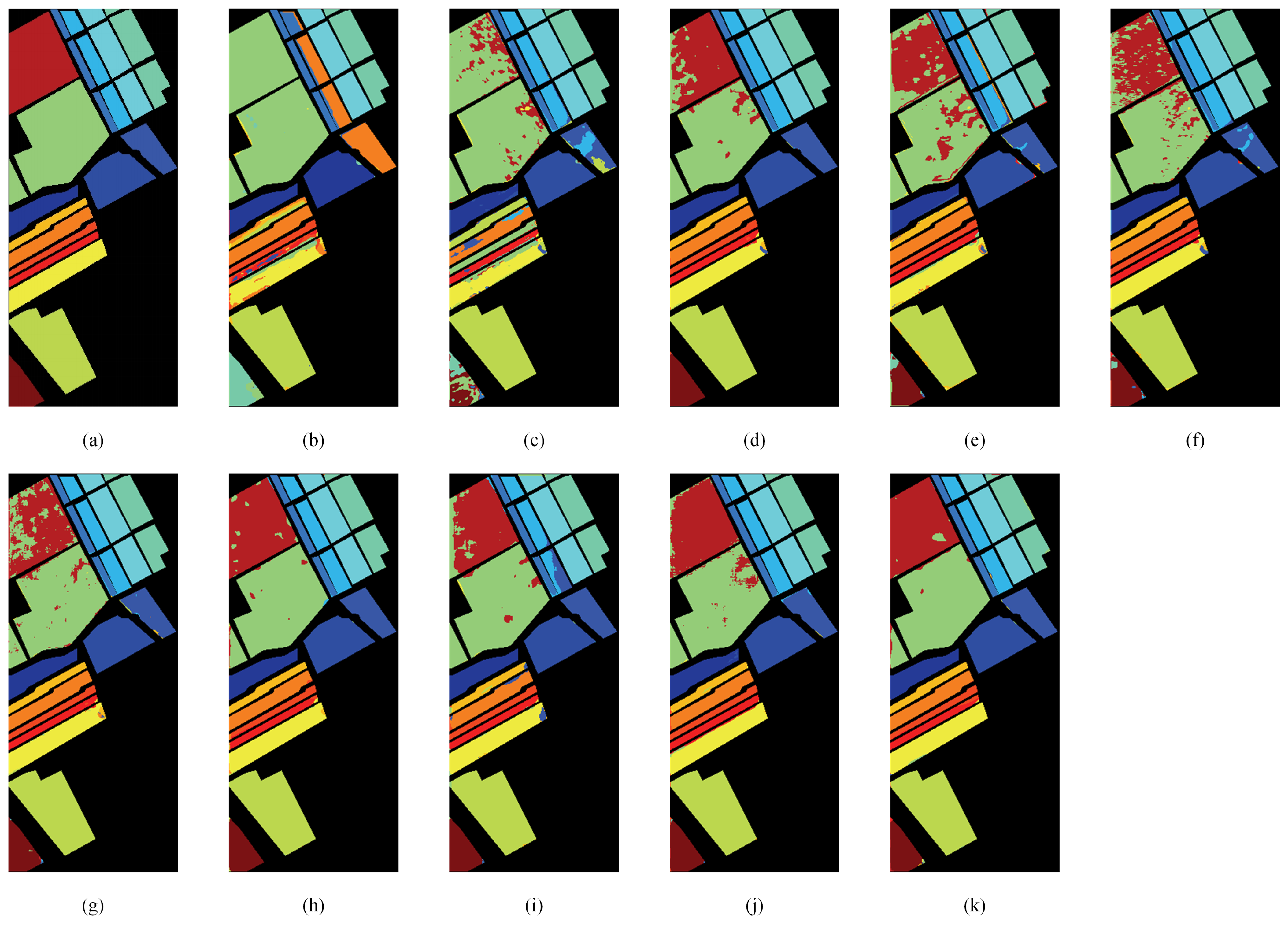
In addition, we present the classification maps of various models in Figure 10, Figure 11 and Figure 12 across the three datasets to concretely demonstrate the classification accuracy of each compared model. From these figures, it is clear that the classification maps produced by SCGHN perform excellently across the three datasets. Compared to other models, the SCGHN maps show substantially less noise and more precisely reflect the ground truth distributions. This conclusively demonstrates that the SCGHN not only achieves high accuracy in real-data classification but also effectively reduces misjudgments and misclassifications, thereby providing more reliable results for classification tasks. These findings robustly validate the practical advantages and effectiveness of the SCGHN.

3.6. Analysis on Model Complexity

Undoubtedly, the advantages of the SCGHN are not limited to classification accuracy. In

Table 10. Complexity comparison of nine models across three datasets (best results are bolded).

	Model	Parameters/K	FLOPs/M	Train Time (s)	Test Time (s)
Salinas	2DCNN	1718.16	57.69	33.25	8.99
	3DCNN	261.70	137.75	14.22	7.85
	SPRN	183.35	9.04	32.32	5.85
	SpectralFormer	352.40	36.43	175.26	27.80
	CAEVT	359.95	123.02	93.57	20.95
	GAHT	972.62	47.61	44.57	8.77
	SSFTT	148.49	11.40	7.65	3.78
	GSC-ViT	104.21	14.89	32.43	13.51
	${\mathrm{S}}^2$Mamba	875.97	91.56	143.61	21.78
	SCGHN	54.88	10.50	8.34	4.59
Pavia University	2DCNN	1484.55	34.41	43.88	13.38
	3DCNN	225.12	91.71	18.88	12.64
	SPRN	178.78	8.86	33.81	8.69
	SpectralFormer	164.39	14.44	239.14	41.84
	CAEVT	206.09	56.35	109.21	20.88
	GAHT	927.11	45.41	54.52	13.28
	SSFTT	148.03	11.40	11.25	7.43
	GSC-ViT	77.90	11.17	37.91	19.34
	${\mathrm{S}}^2$Mamba	408.73	35.92	196.09	34.31
	SCGHN	54.44	5.12	13.85	9.68
WHU-Hi-LongKou	2DCNN	1869.32	72.89	76.19	27.61
	3DCNN	200.98	183.22	23.66	6.90
	SPRN	184.89	9.16	46.91	13.20
	SpectralFormer	540.64	55.02	918.83	83.55
	CAEVT	454.92	166.40	166.09	56.04
	GAHT	1514.12	74.15	75.07	20.28
	SSFTT	148.03	11.40	11.00	7.50
	GSC-ViT	173.06	23.07	61.09	33.96
	${\mathrm{S}}^2$Mamba	1343.89	132.76	753.44	66.51
	SCGHN	54.50	3.15	10.84	6.54

, we list the parameter counts, FLOPs and training/testing time of the SCGHN and compare them with other models on three datasets. In terms of parameters, SCGHN achieves only 54.48 K, 54.44 K and 54.5 K on the Salinas, Pavia University and WHU-Hi-LongKou datasets, significantly fewer than other models. For FLOPs, SCGHN also demonstrates superior performance with values far lower than other models, reflecting its design principle of achieving efficient classification through reduced parameters and computational costs. Although the training time and testing time of SCGHN are not the shortest among all models, they remain advantageous compared to models with similar parameter counts and computational complexity. Overall, SCGHN achieves a balanced performance in model complexity, computational cost and time consumption, ranking among the highest across all compared models on the three datasets.

4. Conclusions and Future Work

This paper proposes a Spectral-Cube Gated Harmony Network (SCGHN) to address the challenge of synergizing global modeling and local feature extraction in hyperspectral image (HSI) classification. The model achieves dynamic gating-based spectral dimension filtering and deformable convolution-based adaptive fusion in the spatial dimension through the Spectral Cooperative Parallel Convolution (SCPC) module, while integrating a cross-scale contextual complementary mechanism through the Dual-Gated Fusion (DGF) module. This design significantly reduces parameter counts while enhancing discriminative capability for mixed land-cover boundaries. Furthermore, the co-design of 3D convolution and a Lightweight Classification Decision module optimizes end-to-end feature representation efficiency. Finally, we compare our model with state-of-the-art classification models on three standard HSI datasets. Comprehensive experimental results demonstrate that our model maintains outstanding classification accuracy while drastically reducing parameters. Although SCGHN excels in classification accuracy and computational efficiency, the following improvements are warranted. First, the model’s sensitivity to hyperparameters suggests future exploration of adaptive parameter optimization strategies to enhance robustness. Second, the current dynamic gating mechanism primarily focuses on spectral–spatial feature interaction while lacking explicit modeling of temporal or 3D structural information—future work may explore multimodal data fusion frameworks to address complex remote sensing scenarios. Third, the real-time processing capability of SCGHN on ultra-large-scale hyperspectral data requires further optimization—combining model compression or hardware acceleration techniques may overcome practical application bottlenecks.

References

1. Yue, J.; Fang, L.; Ghamisi, P.; Xie, W.; Li, J.; Chanussot, J. Optical remote sensing image understanding with weak supervision: Concepts, methods, and perspectives. IEEE Geosci. Remote Sens. Mag. 2022, 10, 250–269. [Google Scholar] [CrossRef]
2. Lee, M.A.; Huang, Y.; Yao, H.; Thomson, S.J.; Bruce, L.M. Determining the effects of storage on cotton and soybean leaf samples for hyperspectral analysis. IEEE J. Sel. Top. Appl. Earth Obs. Remote Sens. 2014, 7, 2562–2570. [Google Scholar] [CrossRef]
3. Chi, J.; Crawford, M.M. Spectral unmixing-based crop residue estimation using hyperspectral remote sensing data: A case study at Purdue university. IEEE J. Sel. Top. Appl. Earth Obs. Remote Sens. 2014, 7, 2531–2539. [Google Scholar] [CrossRef]
4. Sahadevan, A.S. Extraction of spatial-spectral homogeneous patches and fractional abundances for field-scale agriculture monitoring using airborne hyperspectral images. Comput. Electron. Agric. 2021, 188, 106325. [Google Scholar] [CrossRef]
5. Gevaert, C.M.; Suomalainen, J.; Tang, J.; Kooistra, L. Generation of spectral–temporal response surfaces by combining multispectral satellite and hyperspectral UAV imagery for precision agriculture applications. IEEE J. Sel. Top. Appl. Earth Obs. Remote Sens. 2015, 8, 3140–3146. [Google Scholar] [CrossRef]
6. Ryan, J.P.; Davis, C.O.; Tufillaro, N.B.; Kudela, R.M.; Gao, B.C. Application of the hyperspectral imager for the coastal ocean to phytoplankton ecology studies in Monterey Bay, CA, USA. Remote Sens. 2014, 6, 1007–1025. [Google Scholar] [CrossRef]
7. Brook, A.; Dor, E.B. Quantitative detection of settled dust over green canopy using sparse unmixing of airborne hyperspectral data. IEEE J. Sel. Top. Appl. Earth Obs. Remote Sens. 2015, 9, 884–897. [Google Scholar] [CrossRef]
8. Wang, J.; Zhang, L.; Tong, Q.; Sun, X. The Spectral Crust project—Research on new mineral exploration technology. In Proceedings of the 2012 4th Workshop on Hyperspectral Image and Signal Processing: Evolution in Remote Sensing (WHISPERS), Shanghai, China, 4–7 June 2012. [Google Scholar]
9. Lampropoulos, G.A.; Liu, T.; Qian, S.E.; Fei, C. Hyperspectral classification fusion for classifying different military targets. In Proceedings of the IGARSS 2008-2008 IEEE International Geoscience and Remote Sensing Symposium, Boston, MA, USA, 7–11 July 2008. [Google Scholar]
10. Ardouin, J.P.; Lévesque, J.; Rea, T.A. A demonstration of hyperspectral image exploitation for military applications. In Proceedings of the 2007 10th International Conference on Information Fusion, Quebec, QC, Canada, 9–12 July 2007. [Google Scholar]
11. Yuan, J.; Wang, S.; Wu, C.; Xu, Y. Fine-grained classification of urban functional zones and landscape pattern analysis using hyperspectral satellite imagery: A case study of Wuhan. IEEE J. Sel. Top. Appl. Earth Obs. Remote Sens. 2022, 15, 3972–3991. [Google Scholar] [CrossRef]
12. Zhang, C.; Mou, L.; Shan, S.; Zhang, H.; Qi, Y.; Yu, D.; Zhu, X.; Sun, N.; Zheng, X.; Ma, X. Medical hyperspectral image classification based weakly supervised single-image global learning network. Eng. Appl. Artif. Intell. 2024, 133, 108042. [Google Scholar] [CrossRef]
13. Sun, L.; Wu, Z.; Liu, J.; Xiao, L.; Wei, Z. Supervised spectral–spatial hyperspectral image classification with weighted Markov random fields. IEEE Trans. Geosci. Remote Sens. 2014, 53, 1490–1503. [Google Scholar] [CrossRef]
14. Melgani, F.; Bruzzone, L. Classification of hyperspectral remote sensing images with support vector machines. IEEE Trans. Geosci. Remote Sens. 2004, 42, 1778–1790. [Google Scholar] [CrossRef]
15. Archibald, R.; Fann, G. Feature selection and classification of hyperspectral images with support vector machines. IEEE Geosci. Remote Sens. Lett. 2007, 4, 674–677. [Google Scholar] [CrossRef]
16. Fauvel, M.; Benediktsson, J.A.; Chanussot, J.; Sveinsson, J.R. Spectral and spatial classification of hyperspectral data using SVMs and morphological profiles. IEEE Trans. Geosci. Remote Sens. 2008, 46, 3804–3814. [Google Scholar] [CrossRef]
17. Zhuang, L.; Gao, L.; Ni, L.; Zhang, B. An improved expectation maximization algorithm for hyperspectral image classification. In Proceedings of the 2013 5th Workshop on Hyperspectral Image and Signal Processing: Evolution in Remote Sensing (WHISPERS), Gainesville, FL, USA, 26–28 June 2013. [Google Scholar]
18. Feng, W.; Bao, W. Weight-based rotation forest for hyperspectral image classification. IEEE Geosci. Remote Sens. Lett. 2017, 14, 2167–2171. [Google Scholar] [CrossRef]
19. Ma, L.; Crawford, M.M.; Tian, J. Local manifold learning-based k-nearest-neighbor for hyperspectral image classification. IEEE Trans. Geosci. Remote Sens. 2010, 48, 4099–4109. [Google Scholar] [CrossRef]
20. Cai, R.; Liu, C.; Li, J. Efficient phase-induced gabor cube selection and weighted fusion for hyperspectral image classification. Sci. China Technol. Sci. 2022, 65, 778–792. [Google Scholar] [CrossRef]
21. Liang, B.; Liu, C.; Li, J.; Plaza, A.; Bioucas-Dias, J.M. Semisupervised discriminative random field for hyperspectral image classification. IEEE J. Sel. Top. Appl. Earth Obs. Remote Sens. 2021, 14, 12403–12414. [Google Scholar] [CrossRef]
22. Dalla Mura, M.; Villa, A.; Benediktsson, J.A.; Chanussot, J.; Bruzzone, L. Classification of hyperspectral images by using extended morphological attribute profiles and independent component analysis. IEEE Geosci. Remote Sens. Lett. 2010, 8, 542–546. [Google Scholar] [CrossRef]
23. Li, S.; Song, W.; Fang, L.; Chen, Y.; Ghamisi, P.; Benediktsson, J.A. Deep learning for hyperspectral image classification: An overview. IEEE Trans. Geosci. Remote Sens. 2019, 57, 6690–6709. [Google Scholar] [CrossRef]
24. Liu, P.; Li, J.; Wang, L.; He, G. Remote sensing data fusion with generative adversarial networks: State-of-the-art methods and future research directions. IEEE Geosci. Remote Sens. Mag. 2022, 10, 295–328. [Google Scholar] [CrossRef]
25. Hu, W.; Huang, Y.; Wei, L.; Zhang, F.; Li, H. Deep convolutional neural networks for hyperspectral image classification. J. Sens. 2015, 2015, 258619. [Google Scholar] [CrossRef]
26. Lee, H.; Kwon, H. Contextual deep CNN based hyperspectral classification. In Proceedings of the 2016 IEEE International Geoscience and Remote Sensing Symposium (IGARSS), Beijing, China, 10–15 July 2016. [Google Scholar]
27. Chen, Y.; Jiang, H.; Li, C.; Jia, X.; Ghamisi, P. Deep feature extraction and classification of hyperspectral images based on convolutional neural networks. IEEE Trans. Geosci. Remote Sens. 2016, 54, 6232–6251. [Google Scholar] [CrossRef]
28. Zhong, Z.; Li, J.; Luo, Z.; Chapman, M. Spectral–spatial residual network for hyperspectral image classification: A 3-D deep learning framework. IEEE Trans. Geosci. Remote Sens. 2017, 56, 847–858. [Google Scholar] [CrossRef]
29. Howard, A.G.; Zhu, M.; Chen, B.; Kalenichenko, D.; Wang, W.; Weyand, T.; Andreetto, M.; Adam, H. Mobilenets: Efficient convolutional neural networks for mobile vision applications. arXiv 2017, arXiv:1704.04861. [Google Scholar] [CrossRef]
30. Roy, S.K.; Krishna, G.; Dubey, S.R.; Chaudhuri, B.B. HybridSN: Exploring 3-D–2-D CNN feature hierarchy for hyperspectral image classification. IEEE Geosci. Remote Sens. Lett. 2019, 17, 277–281. [Google Scholar] [CrossRef]
31. Zhu, C.; Zhang, T.; Wu, Q.; Li, Y.; Zhong, Q. An implicit transformer-based fusion method for hyperspectral and multispectral remote sensing image. Int. J. Appl. Earth Obs. Geoinf. 2024, 131, 103955. [Google Scholar] [CrossRef]
32. Liu, Y.; Wang, K.; Li, M.; Huang, Y.; Yang, G. A Position-Temporal Awareness Transformer for Remote Sensing Change Detection. IEEE Trans. Geosci. Remote Sens. 2024, 62, 3432320. [Google Scholar] [CrossRef]
33. Sun, L.; Zhao, G.; Zheng, Y.; Wu, Z. Spectral–spatial feature tokenization transformer for hyperspectral image classification. IEEE Trans. Geosci. Remote Sens. 2022, 60, 1–14. [Google Scholar] [CrossRef]
34. Zhao, Z.; Xu, X.; Li, S.; Plaza, A. Hyperspectral image classification using groupwise separable convolutional vision transformer network. IEEE Trans. Geosci. Remote Sens. 2024, 62, 3377610. [Google Scholar] [CrossRef]
35. Chang, Y.; Liu, Q.; Zhang, Y.; Dong, Y. Unsupervised Multi-view Graph Contrastive Feature Learning for Hyperspectral Image Classification. IEEE Trans. Geosci. Remote Sens. 2024, 62, 3431680. [Google Scholar] [CrossRef]
36. Wang, M.; Sun, Y.; Xiang, J.; Sun, R.; Zhong, Y. Joint classification of hyperspectral and LiDAR data based on adaptive gating mechanism and learnable transformer. Remote Sens. 2024, 16, 1080. [Google Scholar] [CrossRef]
37. Guerri, M.F.; Distante, C.; Spagnolo, P.; Taleb-Ahmed, A. Boosting hyperspectral image classification with Gate-Shift-Fuse mechanisms in a novel CNN-Transformer approach. Comput. Electron. Agric. 2025, 237, 110489. [Google Scholar] [CrossRef]
38. Li, S.; Liang, L.; Zhang, S.; Zhang, Y.; Plaza, A.; Wang, X. End-to-end convolutional network and spectral-spatial Transformer architecture for hyperspectral image classification. Remote Sens. 2024, 16, 325. [Google Scholar] [CrossRef]
39. Zhong, Y.; Hu, X.; Luo, C.; Wang, X.; Zhao, J.; Zhang, L. WHU-Hi: UAV-borne hyperspectral with high spatial resolution (H2) benchmark datasets and classifier for precise crop identification based on deep convolutional neural network with CRF. Remote Sens. Environ. 2020, 250, 112012. [Google Scholar] [CrossRef]
40. Tang, X.; Yao, Y.; Ma, J.; Zhang, X.; Yang, Y.; Wang, B.; Jiao, L. SpiralMamba: Spatial-Spectral Complementary Mamba with Spatial Spiral Scan for Hyperspectral Image Classification. IEEE Trans. Geosci. Remote Sens. 2025, 63, 3559137. [Google Scholar] [CrossRef]
41. Li, L.; Ma, H.; Zhang, X.; Zhao, X.; Lv, M.; Jia, Z. Synthetic aperture radar image change detection based on principal component analysis and two-level clustering. Remote Sens. 2024, 16, 1861. [Google Scholar] [CrossRef]
42. Hamida, A.B.; Benoit, A.; Lambert, P.; Amar, C.B. 3-D deep learning approach for remote sensing image classification. IEEE Trans. Geosci. Remote Sens. 2018, 56, 4420–4434. [Google Scholar] [CrossRef]
43. Zhang, X.; Shang, S.; Tang, X.; Feng, J.; Jiao, L. Spectral partitioning residual network with spatial attention mechanism for hyperspectral image classification. IEEE Trans. Geosci. Remote Sens. 2021, 60, 3074196. [Google Scholar] [CrossRef]
44. Hong, D.; Han, Z.; Yao, J.; Gao, L.; Zhang, B.; Plaza, A. SpectralFormer: Rethinking hyperspectral image classification with transformers. IEEE Trans. Geosci. Remote Sens. 2021, 60, 3130716. [Google Scholar] [CrossRef]
45. Zhang, Z.; Li, T.; Tang, X.; Hu, X.; Peng, Y. CAEVT: Convolutional autoencoder meets lightweight vision transformer for hyperspectral image classification. Sensors 2022, 22, 3902. [Google Scholar] [CrossRef] [PubMed]
46. Mei, S.; Song, C.; Ma, M.; Xu, F. Hyperspectral image classification using group-aware hierarchical transformer. IEEE Trans. Geosci. Remote Sens. 2022, 60, 1–14. [Google Scholar] [CrossRef]
47. Wang, G.; Zhang, X.; Peng, Z.; Zhang, T.; Jiao, L. S2Mamba: A spatial-spectral state space model for hyperspectral image classification. IEEE Trans. Geosci. Remote Sens. 2025, 63, 3530993. [Google Scholar] [CrossRef]
Figure 1. Overall framework of the proposed SCGHN model for the HSIC.
Electronics 14 03553 g001
Figure 2. Overall framework of SCPC.
Electronics 14 03553 g002
Figure 3. Overall framework of DGF.
Electronics 14 03553 g003
Figure 4. Salinas dataset. (a) False-color map. (b) Ground-truth map.
Electronics 14 03553 g004
Figure 5. Pavia University dataset. (a) False-color map. (b) Ground-truth map.
Electronics 14 03553 g005
Figure 6. WHU-Hi-LongKou dataset. (a) False-color map. (b) Ground-truth map.
Electronics 14 03553 g006
Figure 7. Impact of different patch size on OA across the three datasets.
Electronics 14 03553 g007
Figure 8. Impact of different batch size on OA across the three datasets.
Electronics 14 03553 g008
Figure 9. Impact of different learning rate on OA across the three datasets.
Electronics 14 03553 g009
Figure 10. Classification maps of various models in the Salinas dataset. (a) Ground-truth map. (b) 2DCNN. (c) 3DCNN. (d) SPRN. (e) SpectralFormer. (f) CAEVT. (g) GAHT. (h) SSFTT. (i) GSC-ViT. (j) S 2 Mamba. (k) SCGHN.
Electronics 14 03553 g010
Figure 11. Classification maps of various models in the Pavia University dataset. (a) Ground-truth map. (b) 2DCNN. (c) 3DCNN. (d) SPRN. (e) SpectralFormer. (f) CAEVT. (g) GAHT. (h) SSFTT. (i) GSC-ViT. (j) S 2 Mamba. (k) SCGHN.
Electronics 14 03553 g011
Figure 12. Classification maps of various models in the WHU-Hi-LongKou dataset. (a) Ground-truth map. (b) 2DCNN. (c) 3DCNN. (d) SPRN. (e) SpectralFormer. (f) CAEVT. (g) GAHT. (h) SSFTT. (i) GSC-ViT. (j) S 2 Mamba. (k) SCGHN.
Electronics 14 03553 g012