CSGI-Net: A Cross-Sample Graph Interaction Network for Multimodal Sentiment Analysis

Abstract

With the widespread application of multimodal data in sentiment analysis, effectively integrating information from different modalities to improve the accuracy and robustness of sentiment analysis has become a critical issue. Although current fusion methods using Transformer architectures have enhanced inter-modal interaction and alignment to some extent, challenges such as the neglect of intra-modal feature complexity and the imbalance in multimodal data optimization limit the full utilization of modality-specific information by multimodal models. To address these challenges, we propose a novel multimodal sentiment analysis model: Cross-Sample Graph Interaction Network (CSGI-Net). Specifically, CSGI-Net facilitates interaction and learning between each sample and its similar samples within the same modality, thereby capturing the common emotional characteristics among similar samples. During the training process, CSGI-Net quantifies and calculates the optimization differences between modalities and dynamically adjusts the optimization amplitude based on these differences, thereby providing under-optimized modalities with more opportunities for improvement. Experimental results demonstrate that CSGI-Net achieves superior performance on two major multimodal sentiment analysis datasets: CMU-MOSI and CMU-MOSEI.

1. Introduction

As social media platforms like TikTok and YouTube evolve, online data has transitioned from purely textual to multimodal forms, including video and audio [1]. This shift has also expanded the data sources for sentiment analysis from unimodal to multimodal. Extracting emotional information from these data is crucial for decision-makers to understand public opinion and make informed decisions. Additionally, multimodal sentiment analysis is particularly significant for the development of artificial intelligence, as it aids in deeply understanding human emotional expression and communication mechanisms, playing a vital role in advancing general-purpose AI.

In the field of multimodal sentiment analysis today, researchers are increasingly focusing on how to effectively integrate information from different modalities within a framework, known as multimodal fusion. Traditional methods, such as RNN-based TFN [2] and MFN [3], integrate information from various modalities by concatenating or summing the feature vectors from different modalities. However, these approaches tend to simplify the interaction and fusion of information across modalities, often overlooking the inherent complexity within each modality [4]. Intra-modality complexity is manifested in various aspects, such as the semantic hierarchy of text, the non-verbal behavioral details in videos, and the tonal variations and emotional intensity in audio. These subtle yet critical characteristics form the deep structure of emotional expression, and simple fusion strategies often fail to accurately capture these fine-grained differences, leading to a model’s inability to fully understand complex emotions [5].

With the rise of Transformers, several new methods have emerged. MulT [6] addresses modality differences effectively by using a unique bi-space learning strategy that simultaneously captures both commonalities and individualities between modalities. MISA [7] improves the multimodal sentiment analysis performance by constructing modality-invariant and modality-specific representations. Self-MM [8] proposes a method that combines self-supervised learning with a weight adjustment strategy to effectively capture both the consistency and disparities of multimodal data. Hou et al. [9] dynamically fused multimodal data using a Cross-modal Enhanced Transformer, aligned non-textual modalities with textual modalities through Text-centered Contrastive Learning, and employed a multimodal output gate to reduce redundant information. Finally, they applied knowledge distillation to enhance model performance, significantly improving the accuracy of multimodal sentiment analysis. Although these methods leverage the advantages of Transformers to enhance inter-modality interaction and alignment, they still overlook the complex structures within each modality and the imbalanced optimization of multimodal data. As a result, models struggle to deeply understand and refine common features, often failing to abstract general emotional patterns from limited training samples, which leads to a significant performance drop when faced with unknown or low-quality data. This highlights the limitations in the model’s generalization ability and its inadequacy in capturing intra-modality common features [10].

One often-overlooked issue when discussing the training of multimodal models is the inconsistency in optimization paths across different modalities. Due to differences in their foundational performance, learning rates, information richness, and noise resilience, modalities experience varying optimization speeds during model training. Faster-optimizing modalities learn effective representations earlier, and their features are more likely to dominate the overall decision during fusion. In contrast, slower-optimizing modalities may not be fully trained and risk becoming marginalized, making it difficult to effectively utilize their unique information. This “dominant modality” phenomenon leads to parameter updates in multimodal models that are biased toward the stronger modalities, creating gradient bias and reducing the model’s focus on other modalities. As a result, this causes an imbalance in optimization across modalities, hindering the model’s ability to fully leverage the unique information of each modality, even though the multimodal model may still outperform unimodal models overall [11].

To address the above issues, we propose the Cross-Sample Graph Interaction Network (CSGI-Net) model, which includes two core modules: Cross-Sample Graph Interaction (CSGI) and Dynamic Optimization Tuning (DOT). As illustrated in Figure 1 (with each sample connected to three similar samples for example), the CSGI module constructs a star-shaped graph for each intra-modal sample, connecting the central node to its similar samples, allowing dynamic adjustment of edge weights based on node similarity differences and adaptively interacting to learn the emotional commonalities among similar samples. This design not only deepens the model’s understanding of emotional features but also enhances its noise-filtering capabilities. The DOT module calculates the optimization differences among modalities during training and dynamically adjusts the optimization extent based on these differences, providing under-optimized modalities with more opportunities for optimization, thus achieving balanced development across modalities.

To validate the effectiveness and superiority of CSGI-Net, we conducted extensive experiments on two key benchmark datasets in the field of multimodal sentiment analysis: CMU-MOSI and CMU-MOSEI. The experimental results demonstrate that CSGI-Net outperforms existing approaches on both datasets, showcasing its superior performance.

Our main contributions in this paper can be summarized as follows:

• We propose a Cross-Sample Graph Interaction Network (CSGI-Net) for multimodal sentiment analysis. This network deeply explores common emotional features by learning the commonalities among similar samples within each modality. During the training process, the optimization differences between modalities are balanced by dynamically controlling the optimization process of each modality.
• We designed a cross-sample interaction graph, which constructs connections between each sample and its similar samples and dynamically adjusts the weights based on the relevance between samples to learn the common features among similar samples within each modality.
• We designed a multimodal dynamic optimization tuning method. By dynamically controlling the optimization process of each modality during training, this method addresses the imbalance in optimization between modalities, significantly enhancing the model’s generalization ability. This module is a highly flexible, pluggable module that can be integrated into existing multimodal frameworks, offering good versatility.
• We conducted comprehensive experiments on the proposed CSGI-Net model using the CMU-MOSI and CMU-MOSEI datasets. The experimental results demonstrate that CSGI-Net performs exceptionally well across most evaluation metrics, achieving outstanding performance on both datasets, which thoroughly validates its effectiveness and superiority.

The structure of this paper is organized as follows: Section 2 provides a review of the relevant literature in the field of multimodal emotion analysis related to this study; Section 3 presents a detailed description of the CSGI-Net framework and the design of its individual modules; Section 4 outlines the experimental setup and validates the proposed framework through a series of experiments; and finally, Section 5 summarizes the research findings and discusses potential directions for future work.

2. Related Work

2.1. Multimodal Sentiment Analysis

With the rise of the new generation of social media, people’s ways of expressing opinions are transitioning from single-text forms to short videos that integrate text, facial expressions, and sound features. This multimedia trend presents new challenges for sentiment analysis, driving development toward deeper multimodal sentiment analysis.

In the exploration of multimodal sentiment analysis (MSA), early fusion strategies were primarily divided into two modes: “early fusion” and “late fusion.” Early fusion involves concatenating data from different modalities (e.g., text, video, and audio) during the initial stages of model construction, which is then fed into unimodal models for feature extraction and sentiment prediction. For example, Yin et al [12] performed the fusion of three modalities using a hierarchical BiLSTM. In the first layer, the audio and visual features are encoded and weighted by the hidden states and confidence scores to obtain the corresponding features. The second layer fuses the features from all three modalities by averaging the weighted confidence scores. On the other hand, late fusion strategies analyze and predict data from each modality individually before aggregating the predictions through weighted averaging based on modality characteristics and the correlation of prediction results. For instance, in the work by Onno K et al. [13], features extracted from each modality are predicted separately, and at the decision layer, the prediction results of all modalities are weighted and averaged based on emotional weights. In recent years, more widely used multi-stage fusion methods have also emerged. For example, in TFN [2], tensor fusion is employed to generate both local and global fused tensors, effectively reducing redundant information.

With the introduction of Transformer [14] by Google, the rapid development of pre-trained models has propelled MSA into a new phase of advancement. During this period, methods in MSA have increasingly focused on leveraging pre-trained models to extract more and higher-quality modality features. For instance, pre-trained BERT [15] has already been utilized in models such as MISA [7], Self-MM [8], and TeCaFN [16] to directly extract features from text.

In previous works, traditional fusion methods often treat multimodal data as a concatenation or projection of features within a single sample, emphasizing alignment and complementarity between modalities while neglecting the emotional similarities between samples. For example, TFN and LMF fuse modality representations through tensor operations, but these operations are limited to within a single sample and lack the ability to model emotional commonalities between similar samples within the same modality, making it difficult to capture local consistency. On the other hand, Transformer-based methods, such as MulT, excel at capturing long-range dependencies and contextual information but tend to focus more on attention along the time or modality dimensions, giving less attention to the structural relationships of emotional similarities between samples. They still do not model the commonalities between samples within the same modality at the structural level.

Therefore, unlike previous methods that model emotions in a simplistic way, our work utilizes Graph Convolutional Networks (GCN), which are better suited for handling non-Euclidean data, to more effectively address the relationships between samples and fully exploit the common emotional information between similar samples within each modality. GCNs handle similarity relationships by constructing a graph structure between samples, using the graph’s topology and node features for efficient learning. This graph structure explicitly models the emotional similarities between samples, allowing the model to focus more on intra-class emotional consistency while maintaining the diversity of modality representations. This approach helps improve the final multimodal emotion recognition performance.

2.2. Graph Convolutional Network

In recent years, Graph Convolutional Networks (GCNs), an emerging data processing technology, have garnered extensive attention and application in both academia and industry due to their excellent performance in addressing non-Euclidean data problems. GCNs have also demonstrated unique advantages in the field of multimodal sentiment analysis.

Yang et al. [17] introduced the Graph Attention Mechanism (GAT) to handle and align non-aligned multimodal language sequences. Huang et al. [18] focused on using graph convolution mechanisms to capture and integrate cross-modal temporal dependencies and emotional features. Xiao et al. [19] further deepened the emotion fusion strategy by employing multi-channel attention graph convolution to ingeniously synthesize emotional information from different modalities. Wan et al.’s [20] research explored the synergy between knowledge graphs and heterogeneous graph convolution, specifically targeting aspect-level multimodal sentiment analysis. Zhao et al. [21] effectively integrated information from various modalities using graph convolution and heterogeneous data fusion techniques. Tan et al. [22] utilized GCNs to fuse multimodal information in image and text sentiment analysis.

As seen in the above works, Graph Convolutional Networks (GCNs) demonstrate unique advantages in areas such as data fusion, feature extraction, and emotion recognition. However, many studies focus too much on inter-modal interaction and fusion, attempting to improve accuracy through the complementarity of cross-modal information, while neglecting the key role of emotional commonalities within the modality itself. For instance, Yang et al. introduced GAT to enhance modality alignment but did not consider emotional commonality within the modality. Huang et al. emphasized cross-modal temporal dependencies and emotional features but similarly overlooked the emotional commonalities within individual modalities. Xiao et al. enhanced emotional fusion across modalities through multi-channel attention graph convolutions but did not deeply explore emotional features within the modality. Wan et al.’s approach, using knowledge graphs and heterogeneous graph convolution, also focused on cross-modal information fusion but failed to address the emotional commonality within modality-specific samples.

Although these methods have achieved certain success in promoting inter-modal fusion, they have not fully utilized the emotional commonality within modalities. In contrast to their approaches, we propose to learn emotional commonalities between similar samples within the same modality through intra-modal cross-sample graph convolutions. This approach allows us to deepen our understanding of emotional features and provides a more holistic way to model emotions.

2.3. Imbalanced Multimodal Optimizing

In the current field of Multimodal Sentiment Analysis (MSA), although multimodal joint training has become the mainstream approach, research by Sun et al. [23] has revealed an important issue: despite increasing the data volume, the performance improvement of most multimodal learning methods remains limited. Building on this, Wang et al. [24] further investigated the inconsistency in the optimization speeds across different modalities during multimodal joint training. They pointed out that the convergence rates of different modalities can vary significantly, and such imbalances may lead to the overall performance of multimodal models not surpassing—or being on par with—that of unimodal models, thereby failing to fully leverage the advantages of multimodal learning.

In response to the issue of optimization imbalance in multimodal learning, researchers have actively explored and proposed various solutions. Among them, Feng et al. [25] introduced external knowledge by leveraging the knowledge embedded in pre-trained models to enhance the training of multimodal models, particularly strengthening unimodal encoders. This approach helps alleviate the optimization discrepancies between modalities and improves overall performance. On the other hand, Wang et al. [24] proposed a gradient mixing strategy based on model overfitting behavior. This strategy dynamically adjusts the gradient contributions between different modalities according to the overfitting phenomena observed during training, thereby achieving optimization balance.

In these studies, although efforts have been made to balance modality optimization to some extent, both of the main solutions still have certain issues. On one hand, Feng et al. enhanced multimodal training using external knowledge from pre-trained models, particularly strengthening the unimodal encoders to alleviate optimization differences between modalities. However, this method could lead to a decrease in the model’s generalization ability. On the other hand, Wang et al. proposed a gradient mixing strategy based on overfitting, dynamically adjusting the gradient contributions of different modalities to achieve optimization balance. However, this method relies on the overfitting phenomenon during training and cannot dynamically adjust optimization differences throughout the entire training process, potentially leading to inaccurate adjustments and failing to fully balance the optimization speeds of each modality.

To address these issues, we propose a multimodal dynamic optimization tuning strategy. Unlike Feng et al.’s reliance on external knowledge to enhance training or Wang et al.’s adjustment based on overfitting, our DOT strategy quantifies and analyzes optimization differences between modalities throughout the entire training process. This allows us to accurately identify and dynamically adjust the optimization speed of each modality, ensuring that every modality is adequately optimized at the appropriate time. This strategy effectively prevents a modality from converging too quickly and hindering overall performance improvement, while also maintaining the model’s strong generalization ability.

3. Methodology

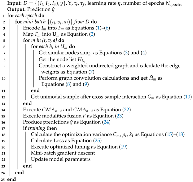
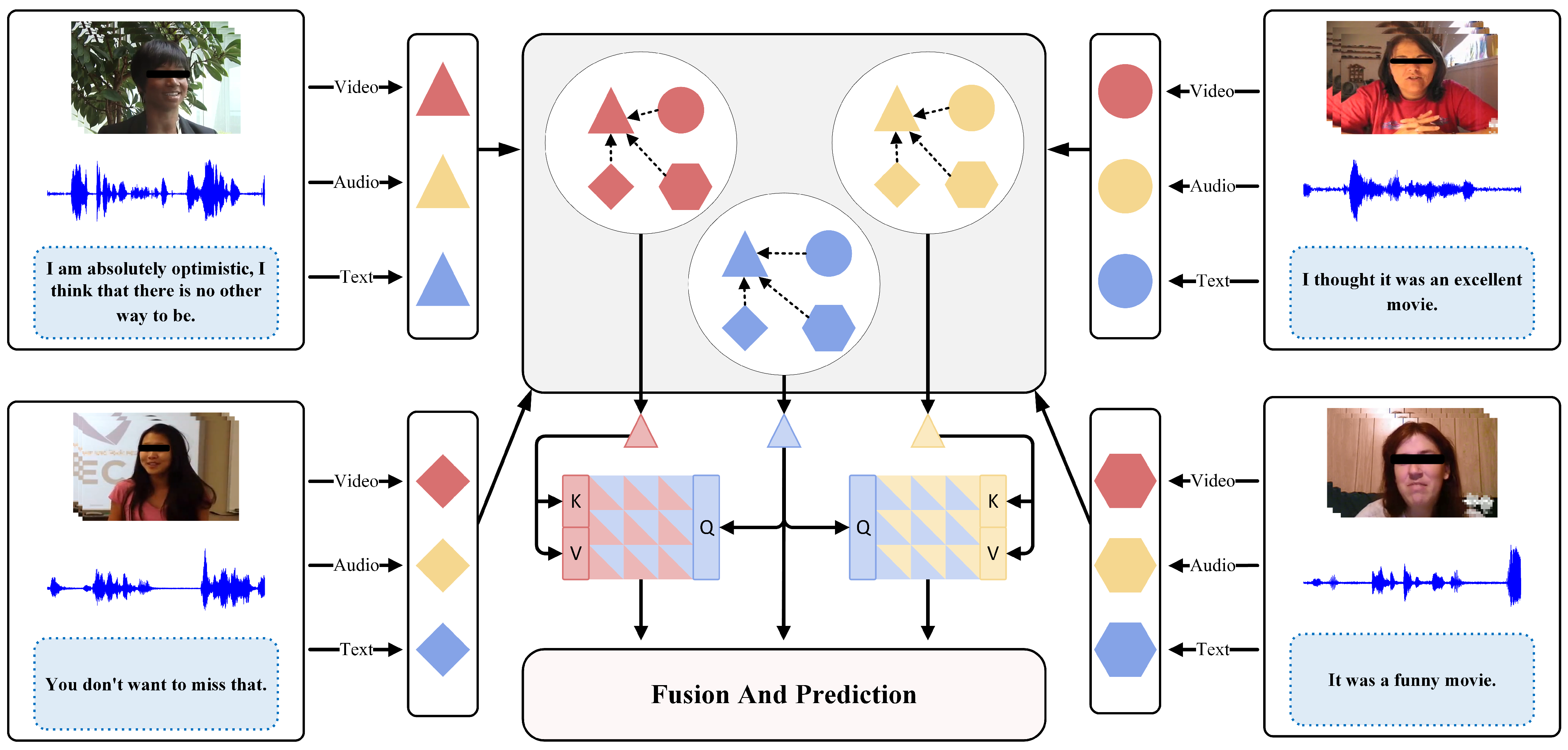
In this section, we will provide a detailed introduction to the proposed Cross-Modal Graph Interaction Network (CSGI-Net). The core objective of CSGI-Net is to capture rich unimodal representations by using graph convolution to learn and extract the common features within each modality among similar samples. Additionally, during the training process, CSGI-Net performs dynamic optimization tuning based on the optimization differences between modalities to ensure that each modality is fully optimized.

3.1. Task Setup

Multimodal Sentiment Analysis (MSA) aims to simultaneously utilize multimodal data (including text $I_t$, video $I_v$, and audio $I_a$) to comprehensively understand and accurately capture the emotional information contained within, revealing deep emotions that are difficult to discover under a single modality. MSA is typically regarded as a regression task or a classification task; in our work, we consider it a regression task. CSGI-Net takes $I_t$, $I_v$, and $I_a$ as the model inputs and ultimately outputs an emotion score $\widehat{y}$. During the model training phase, CSGI-Net has three additional unimodal outputs $C_m$, where $m\in \left\{t,v,a\right\}$, used to calculate the optimization differences between modalities to balance these differences. Although the model has multiple outputs, we only use the final emotion score as the predicted output of the model.

3.2. Overall Architecture

As shown in Figure 2, CSGI-Net consists of four modules: feature extraction, cross-sample graph interaction, dynamic optimization tuning, and modality fusion. The feature extraction module converts the raw multimodal data into vector representations; the cross-sample interaction module learns the common features among similar samples within each modality; the dynamic optimization tuning module adjusts the optimization processes of each modality to reduce optimization imbalances; and the modality fusion module uses text-guided multi-head attention and feature concatenation to fuse features from different modalities for sentiment classification. In this section, we will provide a detailed introduction to these modules.

3.3. Feature Extraction

For the text modality, we utilize the pre-trained language model SentiLARE [26] to extract textual features. Compared to previous models such as BERT [15] and RoBERTa [27], SentiLARE enhances the text feature representation by incorporating external linguistic knowledge through the addition of part-of-speech embeddings and word-level sentiment polarity embeddings into the word embeddings. Based on previous experiences in text modality feature extraction, it is common practice to use the word embedding corresponding to the [CLS] token as the representation of the entire sentence. Therefore, we adopt the same approach to obtain the initial representation ${\mathit{F}}_t$ of the entire sentence:

$${\mathit{F}}_{\mathrm{t}}=SentiLARE\left(I_{\mathrm{t}},{\theta }_{\mathrm{t}}^{SL}\right)\in {\mathbb{R}}^{d_{\mathrm{t}}}$$

(1)

For the video and audio modalities, we use pre-trained OpenFace [28] and COVAREP [29] models to extract initial feature vectors $I_{\mathbf{v}}\in {\mathbb{R}}^{l_{\mathbf{v}}\times d_{\mathbf{v}}};$ and $I_{\mathrm{a}}\in {\mathbb{R}}^{l_{\mathrm{a}}\times d_{\mathrm{a}}}$ from the raw data, where $l_v$ and $l_a$ represent the sequence lengths of the video and audio, respectively. We then employ a bidirectional long short-term memory network (BiLSTM) to capture the contextual temporal characteristics. After processing the entire sequence through the BiLSTM network, we obtain the initial representations ${\mathit{F}}_v$ and ${\mathit{F}}_a$ for the video and audio modalities, respectively.

After obtaining the initial representations for each modality (video, text, and audio), we process this information using modality-specific encoders $Encode{r}_m$. This allows data from different modalities to be unified into a shared semantic space, retaining and enhancing the unique information of each modality to facilitate cross-modal integration. Through this process, the initial modality representations are transformed into the model input ${\mathbf{U}}_m$.

$${\mathbf{U}}_m=Encode{r}_m({\mathit{F}}_m,{\theta }_m^{Encode{r}_m})\in {\mathbb{R}}^{d_{hidden}}$$

(2)

3.4. Cross-Sample Graph Interaction (CSGI)

To enable the model to better capture the shared characteristics among similar samples within the same modality, we constructed a cross-sample interaction graph and applied a custom graph convolution calculation strategy for cross-sample interaction learning. Additionally, during the interaction learning process, our graph dynamically adjusts the edge weights based on the similarity between samples to accurately learn emotional information.

Definition of similar samples: First, we define a new standard for determining similar samples. Previous studies typically considered only semantic similarity while ignoring emotional factors, which led to the learning of irrelevant or even negative information, increasing noise and affecting model performance. Therefore, when defining similar samples, we consider both semantic and emotional similarities.

For semantic similarity, we first normalize the sample representations ${\mathbf{U}}_m$ within each modality, generating the normalized sample representations ${\mathbf{U}}_m^{norm}$ to mitigate the adverse effects of outlier samples. Then, we compute the cosine similarity to construct the semantic similarity matrix ${\mathbf{S}}_m$ between samples within the same modality, reflecting the proximity and correlation of the samples in the semantic space.

For emotional similarity, we employ the external tool NLTK to predict the sentiment of the original sentences. The predicted sentiment labels are then mapped through a linear layer to obtain the generated sentiment label $\tilde{y}$. However, since $\tilde{y}$ is derived from the text modality via an external tool, it may differ from the true label. To address this, we introduce a generation loss ${\mathrm{Loss}}_g$ to align the generated sentiment label $\tilde{y}$ more closely with the true sentiment label y. Subsequently, we compute the emotional difference between samples using the Manhattan distance, constructing the emotional similarity matrix ${\mathbf{E}}_m$, which accurately captures the emotional relationships between samples. By considering both semantic and emotional similarities, we define a more comprehensive notion of similar samples.

$${\mathbf{S}}_m={\displaystyle \frac{{\mathbf{U}}_{m,i}^{\mathrm{norm}}{\mathbf{U}}_{m,j}^{\mathrm{norm}T}}{{∥{\mathbf{U}}_{m,i}^{\mathrm{norm}}∥}_2{∥{\mathbf{U}}_{m,j}^{\mathrm{norm}}∥}_2}}$$

(3)

$${\mathbf{E}}_m=|{\tilde{y}}_i-{\tilde{y}}_o|$$

(4)

In this context, ${\mathbf{S}}_m\in {\mathbb{R}}^{N\times N}$ represents the normalized semantic similarity matrix among samples within each modality in a batch, ${\mathbf{E}}_m\in {\mathbb{R}}^{N\times N}$ denotes the normalized emotional similarity matrix among samples in the batch, $y_i$ indicates the true emotional score of sample i, and $y_o$ represents the true emotional score of each sample, where $i,o\in \{1,2,3,\dots ,N\}$ denote the number of samples.

$${\mathit{F}}_{\mathrm{v}}=BiLSTM\left(I_{\mathrm{v}},{\theta }_{\mathrm{v}}^{BiLSTM}\right)\in {\mathbb{R}}^{d_{\mathrm{v}}}$$

(5)

$${\mathit{F}}_{\mathrm{a}}=BiLSTM\left(I_{\mathrm{a}},{\theta }_{\mathrm{a}}^{BiLSTM}\right)\in {\mathbb{R}}^{d_{\mathrm{a}}}$$

(6)

As shown in Figure 3a, after constructing these two similarity matrices, we define two hyperparameters,${\tau }_{\mathbf{f}}$ and ${\tau }_{\mathbf{s}}$, which represent the thresholds for semantic similarity and emotional similarity, respectively. Using these two hyperparameters, we filter the elements in ${\mathbf{S}}_m$ and generate a sample mask matrix ${\mathbf{M}}_m$. Subsequently, we set the positions in ${\mathbf{S}}_m$ corresponding to False in ${\mathbf{M}}_m$ to negative infinity and select the top K most semantically similar samples for each sample (anchor sample) in the sample sequence, as illustrated in Figure 3b.

Among them, $m\in${ v, t, a } represents the three modalities (video, text, and audio).

Graph Construction: After determining the K similar samples within each modality, we proceed to construct a graph for cross-sample interaction. As shown in Figure 4, we consider four common structures when constructing the graph. Among these, (a) contains a large number of redundant edges, resulting in a significant amount of ineffective computation; (b) and (c) require multiple GCN iterations for the anchor sample to learn the common features of all similar samples, which may lead to learning redundant information; whereas (d) can accurately learn the common features of all similar nodes with just one GCN iteration. Therefore, we choose (d) as the basic model for graph construction.

Specifically, we design a star-shaped weighted undirected graph $\mathcal{G}=(\mathcal{V},\mathcal{E})$ for each sample. The vertex set V has a size of $\left|\mathcal{V}\right|=K+1$, including the anchor sample and its K similar samples. The anchor sample serves as the central node, while the remaining K similar samples are peripheral nodes. The edge set $\mathcal{E}$ has a size of $\left|\mathcal{E}\right|=K$, comprising K edges that represent the similarity relationships between the peripheral nodes and the central node. For three-modal data with N samples, we construct a graph set consisting of three parts, each containing N independent graphs, with each graph designed to have a structure of $K+1$ nodes.

Nodes: Within our model framework, the nodes in the graph are categorized into two major types: ${\mathit{h}}_m^i\in {\mathbf{U}}_m$ and ${\mathit{n}}_m^j\in {\mathbf{sim}}_{h_m^i}$, where $i\in \{1,2,3,\dots ,N\}$, $h_m^i$ represents the i-th sample in modality m($m\in \left\{t,v,a\right\}$) and $j\in \{1,2,3,\dots ,K\}$, ${\mathit{n}}_m^j$ identifies the j-th sample that shows high similarity with sample ${\mathit{h}}_m^i$.

Edges: In our analytical framework, each sample is regarded as a central node in the graph. These central nodes exhibit varying degrees of similarity in semantic features and emotional dimensions with K other samples from the training set. Based on this assumption, we construct a graph model where each central node is connected to its K most similar peripheral nodes. Although there may be some similarity between the similar samples themselves, we focus only on the direct similarity between the central node and its peripheral nodes to avoid introducing unnecessary complexity. Therefore, in the graph, we create edges only between the central node and its specific K similar samples. This ensures the precise capture of the semantic and emotional correlations between samples without blurring the focus by considering all interrelations among similar samples.

Taking a batch of 7 samples as an example, we construct the cross-sample interaction graph for the text modality of the first sample. First, we compute the semantic similarity matrix ${\mathbf{S}}_m$ and the sentiment similarity matrix ${\mathbf{E}}_m$ between these samples, both of which are of size 7 × 7. Then, based on the definition of similar samples, we use the semantic threshold ${\tau }_{\mathbf{f}}$ and sentiment threshold ${\tau }_{\mathbf{s}}$ to filter ${\mathbf{S}}_m$ and ${\mathbf{E}}_m$, masking out the samples that do not meet the criteria. The resulting masks are combined to form the mask matrix ${\mathbf{M}}_m$.

To build the cross-sample interaction graph for the first sample, we extract the first row of ${\mathbf{S}}_m$, ${\mathbf{E}}_m$, and ${\mathbf{M}}_m$, which represent the semantic similarity, sentiment similarity, and similarity mask between the first sample and the other samples, respectively, as shown in Figure 5a. As illustrated in Figure 5a, samples 2 to 5 satisfy the similarity requirements, while samples 6 and 7 are not considered similar to the first sample due to failing to meet both the semantic and sentiment criteria.

Finally, the similarity mask from Figure 5a is used as the first row and first column of the adjacency matrix, with the remaining elements set to 0. This results in the adjacency matrix for the cross-sample interaction graph of the first sample. Based on this adjacency matrix, we obtain the cross-sample interaction graph for the text modality of the first sample, as shown in Figure 5b.

Edge Weights: In our study, we propose a core hypothesis: if two nodes exhibit a high degree of similarity, their shared characteristics become particularly significant, and the weight of the edge between these two nodes needs to be high. To more accurately capture and quantify this similarity between nodes, we introduce cosine similarity [30] as a measurement standard to define the edge weights. By adopting the concept of cosine similarity, we can more precisely depict the strength of the relationships between nodes in complex network analysis. This is especially effective in highlighting the importance of these relationships when there are multiple shared characteristics between nodes. The calculation method for edge weights is as follows:

$${\mathcal{A}}_{ij}^m=1-{\displaystyle \frac{arccos\left(Similarity\left({\mathit{h}}_m^i,{\mathit{n}}_m^j\right)\right)}{\pi }}$$

(7)

where ${\mathit{h}}_m^i$ represents the feature representation of the i-th sample within modality m, and ${\mathit{n}}_m^j$ represents the feature representation of the j-th peripheral node connected to the central node in the graph.

Graph Convolution: Following the aforementioned graph construction steps, we obtain the required weighted undirected graph. We then use this graph to build our custom Graph Convolutional Network (GCN) to further encode and learn the common features among similar nodes. Specifically, given a weighted undirected graph $\mathcal{G}=(\mathcal{V},\mathcal{E})$, let $\mathbf{P}$ be the symmetric normalized Laplacian matrix of the graph $\mathcal{G}$:

$$\begin{array}{cc}\hfill \mathbf{P}& ={\mathbf{D}}^{-{\displaystyle \frac{1}{2}}}\tilde{\mathcal{A}}{\mathbf{D}}^{-{\displaystyle \frac{1}{2}}}\hfill \\ & ={\mathbf{D}}^{-{\displaystyle \frac{1}{2}}}(\mathcal{A}+\mathbf{I}){\mathbf{D}}^{-{\displaystyle \frac{1}{2}}}\hfill \end{array}$$

(8)

where $\mathbf{D}$ represents the degree matrix of graph $\mathcal{G}$, $\mathcal{A}$ represents the adjacency matrix, and I represents the identity matrix. The graph convolution operation we designed can be formulated as:

$$\begin{array}{cc}\hfill {\tilde{\mathbf{H}}}_m^i& ={\mathbf{P}}_m^i{\mathbf{H}}_m^i\hfill \\ \hfill & =\left({{\mathbf{D}}_m^i}^{-{\displaystyle \frac{1}{2}}}{\tilde{\mathcal{A}}}_m^i{{\mathbf{D}}_m^i}^{-{\displaystyle \frac{1}{2}}}\right){\mathbf{H}}_m^i\hfill \end{array}$$

(9)

where the subscript m denotes one of the three modalities (video, text, and audio), and the superscript i represents the cross-sample interaction graph centered on the i-th sample. ${\mathbf{H}}_m^i=\left[{\mathit{h}}_m^i,{\mathit{n}}_m^1,{\mathit{n}}_m^2,\dots ,{\mathit{n}}_m^3\right]\in {\mathbb{R}}^{(K+1)\times d_h}$ represents the feature matrix composed of the features of each node in the graph. Unlike classical graph convolution operations, we discard the conventional learnable weight matrix W. Instead, we implicitly guide the backpropagation process to enhance the learning of common features among similar nodes. This design naturally promotes the network’s information flow to adaptively adjust based on node similarity, eliminating the need for explicit weight parameter adjustments. Consequently, this improves the model’s ability to capture inherent patterns within complex data structures.

Finally, we integrate and reorganize the central node sample ${\mathit{h}}_m^i$ after its interaction with the peripheral nodes, generating a single-modality sample sequence post cross-sample interaction. This sequence is then passed to the subsequent processing stages of the model to further perform downstream tasks.

$${\mathbf{HG}}_m=[{\mathit{h}}_m^1,{\mathit{h}}_m^2,{\mathit{h}}_m^3,\dots ,{\mathit{h}}_m^N]\mathbf{HG}\in {\mathbb{R}}^{N\times d_{hidden}}$$

(10)

3.5. Dynamic Optimization Tuning (DOT)

During the training process of multimodal models, we discovered that the optimization speeds of different modalities are unbalanced. This inconsistency in optimization speeds leads to imbalances in modality optimization during model training, preventing the model from fully utilizing the unique sentimental information contained in each modality and hindering overall performance improvement. To address this issue, we propose a new Dynamic Optimization Tuning (DOT) strategy, aimed at monitoring and responding to the performance fluctuations of each modality in real-time. This strategy dynamically adjusts the optimization intensity allocated to each modality’s feature channels, ensuring that all modalities are adequately optimized.

When employing the GD (Gradient Descent) strategy, the parameters ${\theta }^m$ of the encoder ${\Omega }^m$, where $m\in \left\{v,t,a\right\}$, are updated as follows:

$${\theta }_{\mathrm{s}+1}^m={\theta }_{\mathrm{s}}^m-\eta {\nabla }_{{\theta }^m}L\left({\theta }_{\mathrm{s}}^m\right)$$

(11)

However, in practical applications, the Adam optimization strategy is widely adopted due to its efficiency and robustness. The parameter update rule can be described as follows:

$${\lambda }_{\mathrm{s}}^m={\beta }_1{\lambda }_{\mathrm{s}-1}^m+(1-{\beta }_1)g_{\mathrm{s}}\left({\theta }_{\mathrm{s}}^u\right)$$

(12)

$${\mu }_s^m={\beta }_2{\mu }_{s-1}^m+(1-{\beta }_2)g_s{\left({\theta }_s^u\right)}^2$$

(13)

$${\theta }_{\mathrm{s}+1}^m={\theta }_{\mathrm{s}}^m-{\displaystyle \frac{\alpha }{\sqrt{\frac{{\mu }_{\mathrm{s}}^m}{1-{\beta }_2^s}+ϵ}}}\left({\displaystyle \frac{{\lambda }_{\mathrm{s}}^m}{1-{\beta }_1^t}}\right)$$

(14)

where $g_s\left({\theta }_s^u\right)={\nabla }_{{\theta }^u}L\left({\theta }_s^u\right)$ represents the current gradient, ${\lambda }_{\mathrm{s}}$ and ${\mu }_s$ respectively denote the estimates of the first moment (momentum) and the second moment (variance) at time step s, ${\beta }_1$ and ${\beta }_2$ are hyperparameters used to control the smoothing of the momentum and variance, $\alpha$ is the learning rate, and $ϵ$ is a very small constant (e.g., ${10}^{-8}$), used to prevent division by zero and provide smoothing.

To effectively address the aforementioned issue of imbalances in optimization across modalities, we developed a system of assessment and tuning. The core of this system lies in continuously monitoring and analyzing the differences in learning progress across various modality channels to dynamically adjust the optimization magnitude for each modality. Specifically, we introduce a quantitative metric known as the “single-modality optimization disparity rate”:

$$C_m^s=\sum _{k=1}^N{1}_{k=y_i}·softmax{\left({\mathbf{W}}_s^m·{\phi }_s^m(\theta ,{\mathbf{HG}}_m^s)+{\displaystyle \frac{b}{2}}\right)}_k$$

(15)

$${\rho }_s^{\tilde{m}}={\displaystyle \frac{C_{\tilde{m}}^s}{B_s}}$$

(16)

$${\rho }_s^{\widehat{m}}={\displaystyle \frac{B_s}{\frac{1}{3}{\Sigma }_m^{\{v,t,a\}}{C}_m^s}}$$

(17)

In our method, in order to precisely quantify the performance of a single modality channel, we use ${\mathbf{W}}_s^m·{\phi }_s^m(\theta ,{\mathbf{HG}}_m^s)+{\displaystyle \frac{b}{2}}$ as the approximate predictive value for channel m’s contribution to the target, where ${\mathbf{W}}_s^m$ and ${\phi }_s^m$ represent the weight and feature mapping function of channel m at time step s, respectively; $\theta$ represents the learnable parameters in ${\phi }_s^m$; ${\mathbf{HG}}_m^s$ represents the sequence of samples for modality m at time step s; and b is a bias term. Based on this prediction, we evaluate the performance metric $C_m^s$ for each modality channel m at a given optimization time step in the multimodal model.

Subsequently, by comparing the performance of the video (v), text (t), and audio (a) modality channels, we identify the dominant modality channel at the current time step s as $B_s=max\left(C_m^s\right)$, where $m\in \left\{v,t,a\right\}$, and denote this dominant modality with $\widehat{m}$. To continuously track the performance gap between the non-dominant modalities and the current dominant modality, we introduce a dynamic monitoring metric ${\rho }_s^{\tilde{m}}$, where $\tilde{m}$ represents the modalities other than the one corresponding to $B_s$. Simultaneously, we use ${\rho }_s^{\widehat{m}}$ to measure the extent of advanced optimization of the dominant modality compared to the overall average performance. This ensures appropriate constraints on the dominant modality to prevent overfitting and reduce suppression of the optimization processes in other modalities.

Based on the analysis of performance differences across modalities, we designed a dynamic optimization tuning mechanism aimed at dynamically adjusting the optimization gradient values for each modality channel. This mechanism effectively narrows the optimization gap between different modality channels by:

$$k_s^u=\left\{\begin{array}{cc}1-tanh(\xi ·{\rho }_s^u)& {\rho }_s^u>1\\ 1+{\rho }_s^u& others\end{array}\right.$$

(18)

where $\xi$ is a hyperparameter used to control the extent of gradient tuning, and $u\in \{\widehat{m},\tilde{m}\}$. Unlike using a fixed adjustment function, $\theta$, as a learnable parameter within the model, can automatically learn through training how to allocate appropriate gradient weights between different modalities. When a modality is poorly optimized at a certain stage (e.g., when the loss decreases slowly or gradients are unstable), the model can adjust the corresponding parameter $\theta$ for that modality, increasing the learning rate or enhancing the gradient to provide more optimization focus. Conversely, the model can suppress the gradient update for that modality to prevent overfitting [11]. Therefore, we integrate the optimization difference coefficient $k_s^u$ into the Adam optimization strategy and update the learnable parameters ${\theta }_s^u$ of the encoder ${\Omega }^u$ at the current time step s as follows:

$$\begin{array}{cc}\hfill {\theta }_{s+1}^u& ={\theta }_s^u-\alpha ·k_s^u{\tilde{g}}_s\left({\theta }_s^u\right)\hfill \\ \hfill {\tilde{g}}_s\left({\theta }_s^u\right)& ={\displaystyle \frac{\left(\frac{{\lambda }_s^u}{1-{\beta }_1^s}\right)}{\sqrt{\frac{{\mu }_s^u}{1-{\beta }_2^s}+ϵ}}}\hfill \end{array}$$

(19)

After completing the optimization tuning steps, to prevent the model from becoming trapped in local optima, we incorporate random Gaussian noise into the optimization gradient calculations during training. This disruption of the existing gradient landscape encourages model parameters to escape the constraints of local minima and explore a broader weight configuration space. By doing so, the model can transcend the limitations of local optimization, discover superior solutions in a more extensive parameter space, and thereby enhance its generalization ability on unseen data.

3.6. Modality Fusion and Prediction

3.6.1. Fusion

Although traditional views suggest that text has a significant advantage in conveying emotional information, recent studies indicate that each modality possesses unique value in emotional communication [31]. Therefore, we facilitate cross-modal learning between video and audio modalities guided by the text modality, maximizing the use of emotional consistency across modalities to enhance the complementarity of cross-modal emotional information. Specifically, utilizing the structural integrity and semantic clarity of text, we guide video and audio modalities to achieve deeper alignment and integration during the feature learning process. The i-th head in multi-head attention is calculated as:

$$MHA(\mathit{Q},\mathit{K},\mathit{V})=Concat({\mathit{head}}_1;\dots ;{\mathit{head}}_{n_h}){\mathbf{W}}_o$$

(20)

$${\mathit{head}}_i=Softmax\left({\displaystyle \frac{\left(\mathbf{Q}{\mathbf{W}}_i^{\mathrm{Q}}\right){\left(\mathbf{K}{\mathbf{W}}_i^{\mathrm{K}}\right)}^T}{\sqrt{d_k}}}\right)\left(\mathbf{V}{\mathbf{W}}_i^{\mathrm{V}}\right)$$

(21)

$${\mathit{CMA}}_{m\to \mathrm{t}}=MHA({\mathbf{HG}}_{\mathrm{t}},{\mathbf{HG}}_m,{\mathbf{HG}}_m)m\in \{\mathrm{v},\mathrm{a}\}$$

(22)

where ${\mathbf{W}}^{\mathrm{Q}}$, ${\mathbf{W}}^{\mathrm{K}}$, and ${\mathbf{W}}^{\mathrm{V}}$ represent the weight matrices for different branches in multi-head attention, $n_h$ denotes the number of heads in multi-head attention, and $d_k$ refers to the dimension of cross-modal attention.

Following the textual guidance, we obtain the final feature vectors for the three modalities: ${\mathit{CMA}}_{\mathrm{a}\to \mathrm{t}}$, ${\mathit{CMA}}_{\mathrm{v}\to \mathrm{t}}$, ${\mathbf{HG}}_t$. We concatenate these vectors to form the final feature vector used by the model for prediction:

$$\mathit{F}=Concat({\mathit{CMA}}_{a\to t},{\mathit{CMA}}_{v\to t},{\mathbf{HG}}_t)$$

(23)

3.6.2. Prediction

The predicted values, which range between −3 and 3, represent different emotional intensities. For binary classification tasks, we divide the predicted values into negative and positive numbers to denote two emotional directions (negative and positive). The model’s final prediction $\widehat{y}$ is generated by the output layer $F{C}_{out}$, which consists of a linear layer combined with a ReLU activation function. The final prediction result can be expressed by the formula:

$$\begin{array}{cc}\hfill \widehat{y}& =F{C}_{\mathrm{out}}(\mathit{F},{\theta }^{\mathrm{out}})\hfill \\ & =ReLU({\mathbf{W}}_{\mathrm{out}}\mathit{F}+b_{\mathrm{out}})\hfill \end{array}$$

(24)

3.7. Optimization Objectives

In our model, the loss function is composed of two components: the task loss $Los{s}_{task}$ and the generation loss $Los{s}_g$. Minimizing $Los{s}_{task}$ enables the model’s overall parameters to reach optimal values, while minimizing $Los{s}_g$ ensures that the generated sentiment scores, after mapping, are closer to the true sentiment scores. Since the mean squared error (MSE) is uniformly sensitive to prediction errors and exhibits favorable derivative properties, it has become one of the most commonly used loss functions in many regression problems. Therefore, during the training process, we adopt MSE as the core metric for both loss functions to guide the optimization of the model parameters. For a training dataset containing N samples, the mathematical formulation of the loss function can be expressed as:

$$\begin{array}{cc}\hfill \mathrm{Loss}& =Los{s}_{task}+{\rm Y}Los{s}_g\hfill \\ & =MSE(y_i,{\widehat{y}}_i)+{\rm Y}MSE(y_i,{\tilde{y}}_i)\hfill \\ & ={\displaystyle \frac{1}{N}}\sum _{i=1}^n{(y_i-{\widehat{y}}_i)}^2+{\rm Y}{\displaystyle \frac{1}{N}}\sum _{i=1}^n{(y_i-{\tilde{y}}_i)}^2\hfill \end{array}$$

(25)

Here, $y_i$ represents the true sentiment label of the i-th sample, ${\widehat{y}}_i$ denotes the predicted value of the i-th sample by the model, and ${\tilde{y}}_i$ refers to the generated sentiment label of the i-th sample. ${\rm Y}$ is a hyperparameter that controls the weight of the generation loss. The squared terms ensure that both positive and negative errors are penalized equally, with larger errors leading to more significant penalties. By minimizing the loss function, the model adjusts its parameters to make the predicted values closer to the true sentiment labels, thereby improving prediction accuracy.

Finally, to provide a more intuitive understanding of the training process of CSGI-Net, we summarize it as Algorithm 1.

Algorithm 1: Cross-Sample Graph Interaction Network (CSGI-Net).

4. Experiments

In this section, we provide a detailed description of the experiment design and implementation, which includes the dataset used, the baseline models established, the evaluation metrics selected, the experiments conducted, and the final results obtained.

Section 4.1, Section 4.2, Section 4.3 and Section 4.4 offer a comprehensive overview of the dataset, baseline models, evaluation metrics, and experimental setup, ensuring the rigor and reproducibility of the experiments. In Section 4.5, we present the experiments conducted according to the experimental setup, followed by a thorough comparison with the baseline models. Section 4.6 and Section 4.7 focus on the ablation studies of the model’s functional modules and hyperparameters, systematically evaluating their impact on the overall performance. In Section 4.8, we assess the effect of different modality combinations on the model’s performance, including single-modal, dual-modal, and tri-modal configurations. Finally, in Section 4.9, we provide an intuitive demonstration of CSGI-Net’s prediction performance by randomly selecting five samples.

4.1. Datasets

Our research is conducted on two important benchmark datasets for multimodal sentiment analysis: CMU-MOSI [32] and CMU-MOSEI [33].

CMU-MOSI is an early standard dataset for multimodal sentiment analysis, consisting of 93 YouTube monologue video clips from 89 speakers, with a total of 2198 samples. These videos present speakers’ personal views and emotional depth on topics such as movies. Each utterance is annotated with an emotional score within the range of [−3, 3], where −3 represents extremely negative sentiment and 3 represents extremely positive sentiment.

CMU-MOSEI is an improved version of CMU-MOSI, expanding the number of utterances, speaker diversity, and topic coverage. It follows the same annotation process as CMU-MOSI to ensure consistency and depth across the dataset. CMU-MOSEI is currently one of the largest multimodal sentiment analysis repositories available.

4.2. Baselines

To thoroughly validate the effectiveness of our proposed CSGI-Net, we selected representative classical baseline models and the latest methods that have performed outstandingly in the field of multimodal sentiment analysis. We conducted a systematic and fair comparison of the results using the same datasets and partitioning settings, employing consistent evaluation metrics (such as Accuracy, F1-score, etc.).

TFN [2] focuses on mapping features of different modalities (such as text and image) into a high-dimensional tensor space, followed by applying a series of transformations (including convolution and fully connected layers) to achieve modality interaction and feature fusion.

LMF [34] emphasizes utilizing low-rank representations to integrate data from different sources, such as text, image, or sound. The core idea is to capture the low-dimensional structure shared among modalities through dimensionality reduction techniques, thereby efficiently fusing information.

MulT [6] leverages directed pairwise cross-modal attention to capture the interactions between multimodal sequences at different time steps, and potentially shifts the flow from one modality to another, thereby achieving end-to-end implicit data alignment.

MISA [7] is dedicated to learning common and specific representations from multimodal data. By distinguishing information that is shared and unique to modalities, it enhances the model’s understanding and processing capabilities for data from different sources.

Self-MM [8] focuses on learning specific representations of multiple modalities through self-supervised tasks, improving the model’s understanding and utilization efficiency of each modality feature without explicit supervision signals.

BIMHA [35] introduces an improved multi-head attention mechanism in video-based sentiment analysis, exploring intra-modal, inter-modal, and bimodal interactions through hierarchical fusion. The model includes three multi-head attention units, using multimodal features as source information and bimodal features as target information, effectively enhancing the accuracy and depth of emotion recognition.

PS-Mixer [36] is designed with two vectors, polarity and intensity, optimizing data representation for emotion prediction decisions by distinguishing and fusing the polarity and intensity vectors.

FNENet [37] reduces the granularity gap between linguistic and non-linguistic modalities by vectorizing the non-linguistic modality and integrates non-linguistic information into the pre-trained language model through a sequence fusion mechanism.

${\mathbf{M}}^{\mathbf{3}}$ixup [38] introduces a mixing strategy during the representation learning phase to enhance the robustness of unimodal representations to missing modalities, enabling the model to make accurate predictions even when some modalities are absent.

TMBL [39] enhances interactions and feature fusion among modalities by introducing bimodal and trimodal binding mechanisms and fine-tuning the internal structure of Transformers.

DTN [40] decouples and transforms the common and modality-specific information in multimodal data through an encoder–decoder framework and a relaxed reconstruction strategy.

SeMUL-PCD [41] employs a self-supervised multi-label multimodal knowledge distillation method, which enhances the generalization ability of multi-label emotion recognition across individuals and multimodal data by leveraging collaborative learning and distillation mechanisms between multiple modalities.

4.3. Evaluation Metrics

To evaluate the effectiveness of the CSGI-Net model, we used mean absolute error (MAE) and Pearson’s correlation coefficient (Corr) to assess the discrepancy and relationship between the predicted and actual values. Additionally, F1-score, binary classification accuracy (ACC-2), and multi-class classification accuracy (ACC-7) were introduced to evaluate classification performance. ACC-2 and F1-score were computed using two classification strategies: “negative/non-negative” (with non-negative including both positive and neutral samples) and “negative/positive” (excluding neutral samples). While MAE aims for minimization, higher values are preferred for the other metrics (Corr, F1-score, ACC-2, and ACC-7).

4.4. Experimental Settings

To optimize model efficiency while ensuring prediction accuracy, we chose mean squared error (MSE) as the loss function to guide the model training. For text feature encoding, we employed a pre-trained BERT model and fine-tuned it to fully exploit the deep semantic features of the text. For visual and audio data, we opted for training from scratch, utilizing a Bidirectional Long Short-Term Memory network (BiLSTM) and updating the network parameters using the Adam optimizer, with the goal of obtaining more accurate and robust modality representations.

During the training process, we consistently used a learning rate of 1 × 10⁻⁵ and dynamically adjusted it based on model performance to avoid overfitting or underfitting and promote rapid convergence. To ensure the reproducibility of the experimental results, we set the same random seed before each training session to ensure consistent results across multiple runs. Further training details and specific parameter configurations can be seen in

Table 1. Training setup details.

Hyperparameter	Value
batch size	32
hidden size	128
learning rate	1 × 10−5
learning rate decay ratio	0.5
number of similar nodes	4
feature threshold	0.75
sentiment threshold	0.5
weight of loss	0.2

.

4.5. Results and Comparison

To validate the effectiveness and superiority of the CSGI-Net model, we conducted detailed experimental evaluations on two widely used datasets.

Table 2. Performance ofCSGI-Net on the CMU-MOSI dataset. ACC-2 and F1-score represent “Negative/Non-negative” and “Negative/Positive”, respectively. ↑ indicates that higher values are better, while ↓ indicates that lower values are better. The bolded numbers represent the optimal results for that particular metric. † means that the result is from [16]; ‡ means that the result is from [42].

CMU-MOSI
Models	MAE ↓	Corr ↑	F1-Score ↑	ACC-2 ↑	ACC-7 ↑
TFN †	0.901	0.698	-/80.7	-/80.8	34.9
LMF †	0.917	0.695	-/82.4	-/82.5	33.2
MulT	0.871	0.698	-/82.8	-/83.0	40
MISA †	0.804	0.764	80.77/82.03	80.79/82.10	-
Self-MM ‡	0.717	0.793	82.8/84.6	82.9/84.6	46.4
BIMHA †	0.925	0.671	78.5/80.03	78.57/80.3	36.44
PS-Mixer	0.794	0.748	80.3/82.1	80.3/82.1	44.31
FNENet	0.69	0.805	83.45/85.5	83.53/85.52	48.25
M3ixup	0.9245	0.6776	-/79.78	-/79.66	34.02
TMBL †	0.867	0.762	82.41/84.29	81.78/83.81	36.3
DTN	0.714	0.807	-/86.2	-/86.2	48.1
Ours	0.678	0.82	85.6/87.28	85.55/87.28	45.44

and

Table 3. Performance of CSGI-Net on the CMU-MOSEI dataset. ACC-2 and F1-score represent “Negative/Non-negative” and “Negative/Positive”, respectively. ↑ indicates that higher values are better, while ↓ indicates that lower values are better. The bolded numbers represent the optimal results for that particular metric. † means that the result is from [16]; ‡ means the result is from [42].

CMU-MOSI
Models	MAE ↓	Corr ↑	F1-Score ↑	ACC-2 ↑	ACC-7 ↑
TFN †	0.593	0.7	- /82.1	-/82.5	50.2
LMF †	0.623	0.677	-/82.1	-/82.0	48
MulT	0.58	0.703	-/82.3	-/82.5	51.8
MISA †	0.568	0.724	82.67/83.97	82.59/84.23	-
Self-MM ‡	0.533	0.766	82.8/85.0	82.4/85.0	53.6
BIMHA †	0.559	0.731	83.35/83.5	84.07/83.96	52.11
PS-Mixer	0.537	0.765	83.1/86.1	83.1/86.1	53
FNENet	0.535	0.765	84.3/86.13	84.14/86.3	53.98
M3ixup	0.616	0.672	-/81.49	-/81.80	49
TMBL †	0.545	0.766	84.87/85.92	84.23/85.84	52.4
DTN	0.579	0.788	-/86.3	-/86.3	52.5
SeMUL-PCD	-	-	-/-	-/88.62	-
Ours	0.531	0.774	83.64/86.53	84.44/86.55	54.02

summarize the performance of CSGI-Net and other baseline models on the CMU-MOSI and CMU-MOSEI datasets.

On the CMU-MOSI dataset, CSGI-Net outperforms most models across various metrics. It achieved the lowest MAE of 0.678, indicating the smallest prediction error. For correlation, it obtained a score of 0.82, demonstrating a high level of agreement between the predicted and actual values. The F1-score also reached 87.28, which is the highest among all models. Additionally, CSGI-Net performed strongly on ACC-2 (85.55/87.28), highlighting its robustness in emotion classification tasks. However, compared to other metrics, the ACC-7 score was 45.44, falling short by two percentage points relative to the best-performing model, indicating room for further improvement.

On the CMU-MOSEI dataset, CSGI-Net also performed exceptionally well. It achieved an MAE of 0.531, a Corr of 0.774, and an F1-score of 86.53, all surpassing other models. In terms of ACC-2 (84.44/86.55) and ACC-7 (54.02), it maintained high accuracy, indicating that the model excels not only on the larger and more diverse CMU-MOSEI dataset but also demonstrates good adaptability and generalization on the smaller CMU-MOSI dataset.

Overall, CSGI-Net demonstrates strong multimodal emotion analysis capabilities on both datasets. Although its performance on seven-class classification on CMU-MOSI slightly lags behind that on CMU-MOSEI, it remains highly competitive compared to other models. We speculate that this may be due to the larger size of the CMU-MOSEI dataset, which is five to ten times the size of other datasets and contains richer emotional information. CSGI-Net leverages interactions between similar samples within each modality to enhance performance, thus performing better in seven-class classification on the larger CMU-MOSEI dataset. In contrast, the smaller size and limited emotional data of CMU-MOSI restrict the full potential of CSGI-Net.

4.6. Ablation Study

Our CSGI-Net model primarily consists of two modules: Cross-Sample Graph Interaction (CSGI) and Dynamic Optimization Tuning (DOT).

To validate the necessity of the two key modules in CSGI-Net for multimodal emotion analysis tasks, we designed a comprehensive ablation study and conducted experiments using the CMU-MOSI dataset to thoroughly analyze the contribution of each module to the overall model performance. Specifically, starting from the complete model, we systematically removed different modules to construct several variant models in order to explore how the model performance changes when individual modules are omitted.

Table 4. The experimental results of the ablation study on the CMU-MOSI dataset, where different module contributions were evaluated. “w/o” denotes the removal of specific modules from the complete model. ↑ indicates that higher values are better, while ↓ indicates that lower values are better. The bolded numbers represent the optimal results for that particular metric.

Description	MAE ↓	Corr ↑	F1-Score ↑	ACC-2 ↑
None Modual	0.842	0.755	80.65/82.29	80.61/82.32
CSGI-Net w/o DOT	0.707	0.809	83.11/85.18	83.1/85.21
CSGI-Net w/o CSGI	0.717	0.805	82.5/83.94	82.51/83.99
CSGI-Net w/o tMHA	0.71	0.797	82.34/84.65	82.22/84.6
CSGI-Net	0.678	0.82	85.6/87.28	85.55/87.28

presents a detailed comparison of the performance of the complete CSGI-Net model and its variants based on the CMU-MOSI dataset.

From the analysis of the results, it is clear that after removing the DOT module, the model’s performance declines due to the inability to quantify optimization differences across modalities. As a result, the advantage of one modality can suppress the optimization of others to some extent, preventing the model from fully leveraging emotional information from other modalities, which leads to decreased performance. As shown in Figure 6, to better visualize the impact of the DOT module on the optimization process of individual modalities, we plotted the performance of the visual modality during training in different models. The results show that the performance of the visual modality in a unimodal model is significantly better than in a multimodal model. When the DOT module is included in the multimodal model, its unimodal performance does not reach that of the unimodal model, but it shows a clear improvement compared to when the DOT module is absent, further confirming the effectiveness of the DOT module.

When the CSGI module is removed, the model loses the ability to learn the common features of similar samples within each modality, making it impossible to deeply mine the emotional expression potential of each modality through the emotional commonality between similar samples. This leads to an inability to comprehensively understand and accurately interpret multimodal data, thereby negatively impacting model performance. Compared to the performance degradation after removing the DOT module, the performance drop after removing the CSGI module is more pronounced, indicating the more crucial role of the CSGI module in our model.

Further experiments show that when all modules are removed from the model, the performance further declines, which confirms the importance of each module in enhancing the overall model performance. Additionally, the results indicate that there is a synergistic effect between these two modules, with their interaction improving performance more than the individual effect of each module.

Furthermore, given the unique emotional expression characteristics of each modality [37], we introduced modality-specific cross-modal multi-head attention before fusion to deeply integrate the distinct information from each modality, thereby promoting cross-modal information fusion. Previous studies have generally suggested that the text modality is superior to the visual and audio modalities in terms of the richness and accuracy of emotional information, making it more suitable as a guiding modality in cross-modal fusion. To validate the applicability of this consensus in our model, we conducted systematic experiments on the CMU-MOSI dataset.

The results presented in

Table 5. The experimental results of the ablation study on cross-modal interaction, where different modalities serve as the guiding modality in multi-head attention.↑ indicates that higher values are better, while ↓ indicates that lower values are better. The bolded numbers represent the optimal results for that particular metric.

Dominant Modality	MAE ↓	Corr ↑	F1-Score ↑	ACC-2 ↑
Video	1.46	0.09	52.41/51.38	48.69/47.71
Audio	1.47	0.07	55.06/53.41	46.65/44.97
Text	0.678	0.82	85.6/87.28	85.55/87.28

show that when the text modality is used as the guiding modality, its semantic emotional cues efficiently map to the visual and auditory domains, significantly enhancing the deep interaction and fusion between modalities. In contrast, since the information contained in non-text modalities is generally more ambiguous, using a non-text modality as the guiding modality results in a substantial performance drop, even falling below the performance of the text modality alone. Additionally, in conjunction with the analysis from Table 4, the cross-modal information transfer strategy allows emotional information from the text modality to effectively guide the optimization of visual and auditory features, thereby deepening the model’s overall understanding of multimodal data.

Additionally, since different fusion strategies can impact model performance to varying degrees, we conducted experiments on two common fusion strategies using the CMU-MOSI dataset. The results are shown in

Table 6. The experimental results of the ablation study on different fusion strategies. ↑ indicates that higher values are better, while ↓ indicates that lower values are better. The bolded numbers represent the optimal results for that particular metric.

Fusion Strategy	MAE ↓	Corr ↑	F1-Score ↑	ACC-2 ↑
Add	0.737	0.781	81.6/84.02	81.49/83.99
Cat	0.678	0.82	85.6/87.28	85.55/87.28

. From the experimental findings, it is evident that using the concatenation strategy for modality fusion outperforms the addition strategy across all metrics. This can be attributed to the fact that the concatenation strategy better preserves the information from each modality, allowing for a more effective integration of multimodal data.

Finally, considering that different concatenation orders during modality fusion may lead to fluctuations in model performance, we conducted experiments on this aspect using the CMU-MOSI dataset. The results are shown in

Table 7. The experimental results of the ablation study on different modality concatenation orders. ↑ indicates that higher values are better, while ↓ indicates that lower values are better. The bolded numbers represent the optimal results for that particular metric.

Concat Order	MAE ↓	Corr ↑	F1-Score ↑	ACC-2 ↑
T+V+A	0.694	0.808	83.57/84.9	83.53/84.91
T+A+V	0.698	0.804	83.32/85.83	83.24/85.52
V+T+A	0.684	0.81	84.47/86.1	84.38/86.06
V+A+T	0.694	0.812	83.0/84.61	82.94/84.6
A+T+V	0.686	0.819	83.41/84.89	83.38/84.91
A+V+T	0.678	0.82	85.6/87.28	85.55/87.28

. As indicated by the data, the concatenation order of A+V+T performed the best across all metrics, achieving the lowest MAE (0.678), the highest correlation (0.82), and the highest accuracy and overall performance on ACC-2 (85.55/87.28), ACC-7 (45.44), and F1-score (85.6/87.28). This suggests that combining audio and visual modalities first provides a more complete emotional and contextual background for the text modality, enabling the model to better understand the text and ultimately improving the overall prediction performance.

4.7. Hyperparameter Study

In our model, the number of similar samples (edge nodes) connected to each sample (central node) significantly affects the model’s performance. If the number of similar samples is too small, the central node fails to sufficiently capture the modal commonality, which limits information interaction and fusion. On the other hand, if the number of similar samples is too large, it may lead to information overload, introduce noise, and interfere with the model’s learning, ultimately degrading performance. Therefore, to investigate whether the selected number of similar samples when constructing the intra-modal cross-sample interaction graph is appropriate, we conducted targeted experiments on the CMU-MOSI dataset. The results of the experiments are shown in Figure 7.

From the analysis of the experimental data in Figure 7, it can be observed that as the number of similar samples connected to a sample increases from 2 to 4, the performance metrics of the model improve. When the number of similar samples reaches 4, all metrics except for the correlation (Corr) attain their optimal values, and Corr is also close to its optimal value. However, when the number of similar samples exceeds 4, the performance metrics begin to decrease to varying degrees. Therefore, through a comprehensive evaluation of the metrics, we conclude that the model’s performance is optimal when each sample is connected to 4 similar samples.

In our model, the loss function consists of two components: the task loss and the generation loss. The primary role of the generation loss (denoted as $Los{s}_g$) is to optimize the mapping relationship of sentiment labels, ensuring that the generated sentiment labels $\tilde{y}$ are closer to the true sentiment labels y. To determine an appropriate weight for the generation loss, we conducted experiments on the CMU-MOSI dataset, with the results presented in

Table 8. The impact of different generation loss weights on model performance. ↑ indicates that higher values are better, while ↓ indicates that lower values are better. The bolded numbers represent the optimal results for that particular metric.

Weight	MAE ↓	Corr ↑	F1-Score ↑	ACC-2 ↑
0	0.694	0.808	82.76/84.53	82.46/84.36
0.1	0.695	0.809	82.82/84.57	82.8/84.6
0.2	0.678	0.82	85.6/87.28	85.55/87.28
0.3	0.709	0.805	82.78/84.24	82.8/84.3
0.4	0.708	0.803	82.22/84.03	82.33/84.04

. From the experimental outcomes, it is evident that when relying solely on the task loss without incorporating the generation loss, the generated sentiment labels fail to be accurately mapped. This leads to a significant deviation in the generated sentiment labels, resulting in a noticeable decline in model performance on the sentiment classification task. This phenomenon underscores the importance of the generation loss in the model optimization process. Further experiments reveal that when the weight of the generation loss is set close to 0.2, the model’s performance gradually improves. However, when the weight deviates from 0.2, model performance begins to deteriorate. Therefore, we conclude that setting the generation loss weight to 0.2 yields the best performance across various evaluation metrics. This result validates that a generation loss weight of 0.2 is both reasonable and effective, as it maximizes the optimization of the task loss while maintaining the accuracy of the generated labels.

In addition to experimenting with these two hyperparameters, we also conducted a systematic analysis of other hyperparameters in the model on the CMU-MOSI dataset to ensure the appropriateness of all hyperparameter settings.

As shown in Figure 8, the model exhibits varying performance under different parameter settings across a series of experiments. In the sentiment similarity threshold experiment, the model achieved the lowest error and highest accuracy when the threshold was set to 0.5, indicating that this threshold setting effectively improves the model’s performance in sentiment recognition tasks. In the semantic similarity threshold experiment, the model reached optimal performance in both error and accuracy when the threshold was set to 0.75, suggesting that this setting more precisely captures semantic similarity, thereby enhancing overall performance.

In the learning rate experiment, the model achieved the best balance between error and accuracy when the learning rate was set to 1 × 10⁻⁵. This indicates that this learning rate not only facilitates stable convergence but also significantly improves overall performance. A smaller learning rate ensures smoother parameter updates during training, thus preventing issues such as gradient explosion or oscillation, and helps the model converge to a better local minimum. Moreover, the choice of learning rate must also consider the trade-off between training time and effectiveness; 1 × 10⁻⁵ is an ideal choice, as it allows the model to gradually optimize over a longer training period, leading to accurate sentiment label predictions and efficient model convergence.

Additionally, we conducted extensive experiments to examine the impact of different batch sizes on model performance. On the CMU-MOSI dataset, the model performed best with a batch size of 32, achieving the lowest MAE and highest accuracy. Compared to larger batch sizes, smaller batch sizes allow more frequent updates during each training step, leading to a finer optimization process that enhances the model’s convergence speed and accuracy. Increasing or decreasing the batch size did not result in improved performance and instead led to slight degradation. This may be due to the fact that a larger batch size slows down parameter updates during each iteration, which impacts the flexibility of the learning process. Conversely, a smaller batch size may introduce more noise during training, compromising model stability. Therefore, a batch size of 32 is considered the optimal choice, as it provides the best balance between error, accuracy, and convergence while also ensuring faster training speeds and higher precision in practical applications.

4.8. Modality Study

Finally, to further investigate the impact of missing different modalities on the performance of the CSGI-Net multimodal model, we conducted experiments on the CMU-MOSI dataset. These experiments explored how the model’s performance changes under conditions where different modalities are missing. Since cross-modal interactions in our proposed model rely on textual information as guidance, we primarily considered scenarios where the video and audio modalities were missing.

The experimental results, as shown in

Table 9. The impact of modal absence on model performance. ↑ indicates that higher values are better, while ↓ indicates that lower values are better. The bolded numbers represent the optimal results for that particular metric.

Description	MAE ↓	Corr ↑	F1-Score ↑	ACC-2 ↑
only text	0.853	0.737	79.84/81.15	79.88/81.25
w/o video	0.697	0.809	82.02/84.32	81.92/84.3
w/o audio	0.686	0.814	83.6/85.68	83.53/85.67
all modality	0.678	0.82	85.6/87.28	85.55/87.28

, reveal that when the video modality is missing, CSGI-Net’s performance is significantly affected, particularly in metrics such as MAE and F1-score, where the model shows a notable decline. This indicates that the video modality plays a crucial role in the sentiment analysis process of the model. In contrast, the absence of the audio modality has a relatively smaller impact on model performance, especially in evaluation metrics such as F1-score and ACC-2, where the model maintains relatively high accuracy.

However, when both the video and audio modalities are missing, leaving only the textual modality, the model’s performance deteriorates significantly due to the absence of emotional information provided by the other modalities, reaching its lowest level. This result further validates the complementary nature of multimodal information, suggesting that a single modality alone cannot adequately capture the multidimensional nature of emotional expression.

Overall, the experiments demonstrate that all modalities and their combinations contribute significantly to the overall performance of CSGI-Net, particularly in key metrics such as MAE, F1-score, and ACC-2, where the model’s predictive capability is effectively enhanced. These findings strongly support the complementary and synergistic role of multimodal information, which plays a crucial part in sentiment analysis tasks.

4.9. Case Study

To visually demonstrate the superior performance of CSGI-Net in multimodal sentiment analysis, we randomly selected five samples for presentation. Each sample includes text, visual, and audio inputs, along with the corresponding predicted sentiment scores and ground truth sentiment scores. These elements are presented in a visual format in Figure 9. Different colors are used in the figure to represent sentiment polarity: red indicates negative emotions, white represents neutral or no significant emotion, and green signifies positive emotions. The intensity of the color reflects the strength of the sentiment: darker colors correspond to stronger emotional expressions, while lighter colors indicate milder emotional expressions.

In the second example, the speaker is smiling, with significant fluctuations in the voice, while the text shows no strong emotional tone. Most sentiment analysis models would classify this as positive sentiment. However, CSGI-Net delves deeper into the emotional commonalities through the interactions between similar samples within each modality, thereby enhancing the emotional information of each modality. As a result, even in ambiguous emotional recognition scenarios, the model can capture unique emotional details. Ultimately, the multimodal output processed by CSGI-Net yields a sentiment score of −0.94442, clearly indicating negative sentiment, with only a 0.05558 difference from the ground-truth sentiment value.

In the third example, the speaker smiles, with notable fluctuations in the voice, and the text shows no clear emotional inclination. Even in this complex scenario, CSGI-Net accurately predicts the sentiment, with a sentiment score that deviates by only 0.03324 from the ground truth, both pointing to a neutral emotion. This demonstrates the importance of commonality learning between similar samples within each modality for improving sentiment analysis accuracy, particularly in cases in which emotional boundaries are blurred.

In the fourth example, the speaker’s facial expression is neutral, with no obvious emotion in the text, but there are significant fluctuations in the voice. Traditional multimodal sentiment analysis models often overlook the potential emotional cues in the audio modality. However, CSGI-Net’s inter-modality optimization and differential balancing mechanism ensure that the audio modality is weighted equally with the visual and text modalities in the model. As a result, the model predicts a positive emotion with a sentiment score of 0.30079, with only a 0.03254 difference from the ground truth, accurately identifying the positive sentiment in the example.

5. Discussion

5.1. Summary of Contributions

The Cross-Sample Graph Interaction Network (CSGI-Net) proposed in this paper aims to address two long-standing yet underappreciated issues in multimodal sentiment analysis tasks: first, the lack of structured modeling between features within a modality, which makes it difficult to effectively capture emotional commonalities; and second, the mismatch in optimization speeds during multimodal training, resulting in an imbalance in modality learning. To tackle these issues, this paper introduces two key modules: the Cross-Sample Graph Interaction (CSGI) module and the Dynamic Optimization Tuning (DOT) module. The former constructs a graph structure between similar samples within a modality to guide the model in perceiving emotional commonality, while the latter dynamically monitors the optimization progress of modalities during training and adjusts the gradient update direction and magnitude in real time, thereby enhancing the collaborative ability of the modalities.

On the standard datasets CMU-MOSI and CMU-MOSEI, CSGI-Net achieves leading results on core metrics such as MAE, Corr, F1-score, and ACC-2. Specifically, the F1-score for the “negative/positive” binary classification task reaches 87.28 and 86.53, respectively, while the MAE remains at a low level, demonstrating CSGI-Net’s strong performance and generalization ability in both regression and classification tasks.

5.2. Comparative Analysis with Prior Literature

In existing multimodal sentiment analysis research, methods like TFN [2] and LMF [34] primarily rely on feature fusion mechanisms between modalities, with a relatively shallow use of internal modality structures, making it difficult to capture complex emotional expression relationships. On the other hand, Transformer-based frameworks such as MulT [6], MISA [7], and Self-MM [8] emphasize cross-modal alignment and shared-specific modeling but generally overlook the potential value of emotional commonality between samples and fail to model and regulate optimization differences between modalities.

In comparison to these methods, CSGI-Net achieves substantial breakthroughs on two fronts: first, in terms of modality internal structural modeling, the CSGI module introduces cross-sample graph structures for the first time. It not only combines semantic and emotional similarities but also leverages graph convolution to learn and extract local sample commonalities, providing structural supplementary information for emotion prediction. Second, in dynamic training modeling, the DOT module monitors and adjusts the optimization magnitude of each modality throughout the training process, effectively alleviating the issue of strong modalities dominating and weak modalities being suppressed—a mechanism that has rarely been addressed in previous studies.

Experimental results show that CSGI-Net achieves breakthroughs across multiple datasets and evaluation dimensions compared to the aforementioned methods. For instance, compared to Self-MM [8], CSGI-Net improves the F1-score by nearly 3 percentage points and reduces the MAE by 0.039 on the CMU-MOSI dataset. Compared to MulT [6], CSGI-Net increases the ACC-7 by about 2.2 percentage points on the CMU-MOSEI dataset, further validating the model’s ability to model the complex interactive relationships between modalities.

5.3. Limitations and Deficiencies

Although CSGI-Net achieved good results in both structural design and experimental performance, it still faces the following potential limitations. The CSGI module relies on semantic structures and the number of samples, necessitating the construction of high-quality, similar sample graphs. Therefore, it is dependent on the data scale and semantic consistency. In scenarios with small sample sizes or strong sample heterogeneity, it becomes difficult to construct stable graph structures, which may impact model performance. Additionally, the training cost is high, and scalability is limited. The graph construction across samples and the graph convolution computation introduce significant computational overhead, especially in large-scale datasets or online inference scenarios, where training and deployment efficiency still leave room for improvement. The modality adjustment mechanism becomes unstable in extreme scenarios. The DOT module may experience gradient adjustment imbalance when the number of modalities is small or when one modality is extremely strong or weak, resulting in the model over-relying on or neglecting certain modalities.

5.4. Remedial Strategies

To address the aforementioned limitations, the following potential solutions are proposed. For the issue of graph structure dependence, future work could introduce graph generation methods based on self-supervised learning or meta-learning to automatically construct stable, similar sample graphs, thus reducing reliance on sample size and labels. To alleviate the training cost problem, alternative solutions for graph convolution, such as Graph Attention Networks (GATs) or lightweight graph encoding modules (e.g., GraphSAGE), could be explored to improve model efficiency. Regarding the instability of the modality adjustment mechanism, a modality credibility evaluation mechanism could be introduced, dynamically adjusting the modality weights based on the quality of the input data, rather than solely relying on performance evaluation results during training. Additionally, the introduction of modality missing robustness mechanisms, such as DropModality or modality reconstruction networks, could further enhance the model’s robustness in real-world scenarios.

5.5. Future Work

Future research could explore the following directions. One potential avenue is task transfer and multi-task learning with CSGI-Net, extending its application to other multimodal tasks such as emotion recognition, stance detection, or multimodal question answering, and examining the adaptability of the graph interaction mechanism across a wider range of tasks. Currently, similar sample graph construction primarily relies on static thresholds; in the future, dynamic graph learning mechanisms could be introduced, or more complex cross-sample relationship modeling could be explored by combining attention mechanisms to learn edge weights and adapt to dynamic changes. By incorporating strategies like cross-domain contrastive learning and domain-invariant encoders, the model could better transfer across different corpus domains, enhancing its applicability and cross-domain generalization capability. Additionally, integrating pre-trained large language models (e.g., ChatGPT and Gemini) with the CSGI module could empower graph structure learning with stronger semantic expression and knowledge transfer capabilities.

6. Conclusions and Future Work

The core challenge in multimodal sentiment analysis lies in how to effectively integrate and leverage emotional information from various modalities. Traditional approaches often focus on cross-modal interaction, frequently overlooking the potential of intra-modal information, especially when the optimization steps across modalities are misaligned, leading to imbalanced training and compromised performance. To address this, we propose CSGI-Net, which introduces the Cross-Modal Graph Interaction (CSGI) module to construct interaction graphs between similar samples within each modality, uncovering common emotional patterns. Additionally, the Dynamic Optimization Tuning (DOT) module is designed to dynamically adjust the optimization pace between modalities, facilitating more coordinated multimodal learning. Experimental results show that CSGI-Net achieves outstanding performance on the CMU-MOSI and CMU-MOSEI datasets, demonstrating the method’s advanced nature and practical value.

Despite CSGI-Net’s strong performance in experiments, there remains room for optimization. On one hand, the model relies on emotional commonality between similar samples, which may affect performance when samples are scarce or when emotional distribution is uneven. On the other hand, the DOT strategy may excessively suppress strong modalities in scenarios with fewer modalities, thus weakening predictive capability. Furthermore, the computational and storage overhead introduced by cross-sample graph construction also poses challenges for large-scale applications.

In the future, we plan to further optimize the DOT strategy to enhance its adaptability in scenarios with limited modalities. We will also improve the graph construction mechanism to balance model performance and efficiency. Moreover, we aim to continue expanding the model’s applicability and robustness, enabling it to unleash greater potential in a wider range of multimodal scenarios.