Article

A Novel Wind Turbine Clutter Detection Algorithm for Weather Radar Data

1
School of Integrated Circuit Science and Engineering, University of Electronic Science and Technology of China, Chengdu 611731, China
2
College of Electronic Eingineering, Chengdu University of Information Technology, Chengdu 610225, China
3
CMA Key Laboratory of Atmospheric Sounding, Chengdu 610225, China
*
Author to whom correspondence should be addressed.
Electronics 2025, 14(17), 3467; https://doi.org/10.3390/electronics14173467
Submission received: 16 July 2025 / Revised: 21 August 2025 / Accepted: 27 August 2025 / Published: 29 August 2025

Abstract

Wind turbine radar echoes exhibit significant scattering power and Doppler spectrum broadening effects, which can interfere with the detection of meteorological targets and subsequently impact weather prediction and disaster warning decisions. In operational weather radar applications, the influence of wind farm on radar observations must be fully considered by meteorological departments and related institutions. In this paper, a Wind Turbine Clutter Classification Algorithm based on Random Forest (WTCDA-RF) classification is proposed. The level-II radar data is processed in blocks, and the spatial position invariance of wind farm clutter is leveraged for feature extraction. Samples are labeled based on position information, and valid samples are screened and saved to construct a vector sample set of wind farm clutter. Through training and optimization, the proposed WTCDA-RF model achieves an ACC of 90.92%, a PRE of 89.37%, a POD of 92.89%, and an F1-score of 91.10%, with a CSI of 83.65% and a FAR of only 10.63%. This not only enhances the accuracy of weather forecasts and ensures the reliability of radar data but also provides operational conditions for subsequent clutter removal, improves disaster warning capabilities, and ensures timely and accurate warning information under extreme weather conditions.

1. Introduction

Wind energy is abundant worldwide and plays a strategic role in achieving carbon neutrality [1]. Since China’s dual-carbon strategy was announced in 2020 [2], wind power has shown strong growth potential. The Global Wind Energy Council (GWEC) released its Global Wind Report 2023 in Sao Paulo, Brazil, projecting that global capacity will exceed 100 GW by 2024 and offshore installations will reach 25 GW by 2025 [3].
Modern wind turbines, often reaching heights of up to 250 m and arranged in dense onshore or offshore clusters [4], have expanded rapidly alongside the global growth of wind power. This large-scale deployment, particularly offshore, poses notable challenges for weather radar systems in atmospheric detection. Interference from rotating blades can degrade radar data quality and undermine early warning capabilities [5]. Unlike fixed structures such as masts or towers, wind turbines produce stronger and more complex echoes [6], which can overlap with meteorological signals and cause misinterpretation of weather phenomena [7]. Furthermore, forward scattering from wind farms can introduce attenuation, multiple scattering, and Doppler contamination into radar measurements [8], while the increasing density of installations exacerbates classification difficulties and multi-target tracking errors, ultimately reducing the accuracy of radar-based detection and recognition [9].
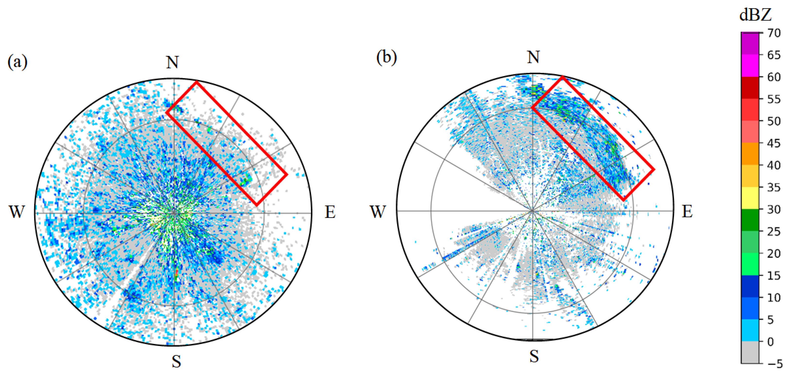
Clutter in weather radar refers to non-meteorological echoes originating from terrain, man-made structures, insects, birds, aircraft, or drones. It is generally categorized into two types: static and dynamic [10]. Static clutter, produced by stationary objects such as wind turbine towers and nacelles, typically exhibits near-zero radial velocity and can often be mitigated with clutter filters. In contrast, dynamic clutter, generated by moving targets such as rotating wind turbine blades, exhibits radial velocities that exceed the threshold of clutter filters, making it more difficult to suppress. Wind turbine clutter (WTC) can closely resemble weather-related signals in terms of power and spectral characteristics, thereby complicating its identification in Plan Position Indicator (PPI) radar observations [11]. These unwanted echoes can significantly degrade radar detection performance. Figure 1 illustrates WTC observed in the 0.5° and 1.5° elevation reflectivity data from CINRAD near Nantong Airport in Nantong City. As shown in the left panel, pronounced clutter interference appears over the northern coastal area at the 0.5° elevation, whereas no clutter is evident at 1.5°. This difference occurs because WTC impacts are typically confined to regions near the ground. A similar distribution has been reported in the United States, where examples from the WSR-88D KDDC radar near Dodge City, Kansas, also demonstrate WTC in 0.5° elevation reflectivity [6]. Figure 2 compares the changes in the distribution of WTCs observed by CINRAD in Nantong City in 2008 and 2025, under clear weather conditions. It can be seen that the WTC in the coastal area began to increase significantly, and seriously affected the detection and identification of weather targets, with the construction of a large number of wind turbines on the coast of Nantong City after 2008.
Differentiating between isolated storm cells and WTC in such mixed scenarios is challenging. WTC not only causes visual interference but also introduces bias into downstream products derived from contaminated radar data. As shown in Figure 3, wind turbine echoes (red circles) are difficult to distinguish from strong storm echoes due to their high radar reflectivity, which can cause large errors in the identification of strong convective cells and quantitative precipitation estimates in weather forecasts. Vogt’s research results found that even if there are only a few turbines near the radar, it will have a significant impact on radar observations [12].
Weather radar is essential for monitoring precipitation, wind shear, and hazardous weather phenomena like hail, heavy rain, and tornadoes. Meteorologists depend on radar data for real-time weather tracking, numerical weather prediction models [13], and hydrological models [14]. Clutter in radar data can influence the generation of radar products and impact forecast systems [15]. Several studies have shown that wind turbines can create detectable false echoes in weather radar data [16,17], and others used American S-band radar data to confirm the presence of wind turbine false echoes in three Doppler spectrum moments: reflectivity, velocity, and spectral width. Ref. [18] conducted detailed studies using a mobile X-band Doppler radar, revealing that multipath scattering predominates on clear sky days, while isolated velocity couplets are more common during precipitation events. They also noted that the radar echo from turbines can be influenced by wind direction and blade angle of attack, affecting the relative motion of the blades within the radar beam. Ref. [19] explored this using long-term Swedish C-band radar data. Subsequently, Ref. [20] used pre and post-construction data to analyze the impact of wind farms on all three Doppler spectral moments. Their study showed significant effects from wind turbines on radar data over a large area near and downstream of the wind farm, even at altitudes up to 3 km above sea level.
Some methods have been proposed to detect and suppress WTC, addressing the problem of interference in weather radar data caused by WTC. Ref. [21] proposed a frequency domain-based algorithm using wind turbines’ large radar scattering cross-section and significant Doppler frequency shift. Ref. [22] utilized range-Doppler domain signal processing to mitigate wind turbine impacts. Despite their promise, distinguishing wind turbine clutter spectra from precipitation echo spectra remains challenging. Ref. [23] applied a fuzzy logic method to automatically detect wind turbine clutter in radar echo time-domain data. Ref. [24] combined reflectivity, Doppler velocity, and spectral width from level-II radar data with a Fuzzy Inference System (FIS) to identify wind turbine clutter under typical meteorological conditions. Ref. [25] leveraged the newly enhanced dual-polarization capabilities to develop a fully automated and physically meaningful polarization algorithm. This algorithm is designed to identify and eliminate non-meteorological radar echoes caused by anomalous beam propagation and wind turbine effects. It effectively mitigates the impact of interactions between anomalous radar beam propagation and distant wind turbines on radar-based precipitation estimates. Building on this, ref. [26] used probability distribution histograms and one-dimensional range distributions to define membership functions and logic rules for adaptive clutter identification. Ref. [27] studied the impact of point targets, such as masts and wind turbines, on in-phase and quadrature-phase (I/Q) data. The study found that normalized amplitude effects of point targets on radar pulses are distinct and repeatable, independent of the wind turbine’s characteristics, and can be filtered out in radar signal processors to improve data robustness. Ref. [28] analyzed radar-based data characteristics, focusing on high reflectivity factor bulges, horizontal channel signal-to-noise ratio bulges, and significant velocity singularities. Their fuzzy logic algorithm, based on statistical results from these features, identifies wind turbine clutter in radar basedata. Compared to He Weikun’s method, Su Tianji’s approach uses fewer features, is less complex, and is more time-efficient.
Existing research focuses on analyzing the radar back reflection characteristics of WTC for identification, focusing on the importance of feature selection and evaluation. However, there is little research on WTC identification algorithms based on weather radar data commonly used in weather forecasting. In this study, a WTC detection algorithm based on Random Forest (WTCDA-RF) is proposed, incorporating three main innovations. First, it applies machine learning techniques to level-II weather radar data products for WTC detection, an application scenario that has been rarely explored. Second, it integrates dual-polarization radar products—including reflectivity, radial velocity, velocity spectrum width, differential reflectivity, differential phase shift rate, and correlation coefficient—allowing for more accurate WTC discrimination than methods relying solely on single-polarization data. Third, it employs feature engineering specifically designed for the physical and operational characteristics of wind turbines to extract spatial and physical descriptors that enhance detection performance. The algorithm processes level-II dual-polarization radar data from Nantong City, segments them into blocks, extracts WTC features for each radar product to build a labeled WTC dataset, and then applies a Random Forest classifier to achieve accurate WTC identification with a low false alarm rate. Finally, the trained WTC recognition model was then applied to Shangchuan Island, characterized by offshore wind turbines, and Changsha, dominated by land-based wind turbines, to evaluate its effectiveness and generalization capability. Experimental results indicate that WTCDA-RF can effectively identify WTC in radar data under various weather conditions, providing a reliable detection method for subsequent WTC removal.

2. Data

2.1. Jiangsu Nantong Weather Radar Data

In 2023, the Comprehensive Observation Department of the China Meteorological Administration upgraded the Nantong CINRAD-SA to a dual-polarization weather radar and incorporated it into the National Refined Radar Observation Pilot Program. Following the upgrade, the radar retained its original volume scan configuration while adding four new refined volume scan modes by default (details are provided in Table 1). The upgraded system offers significantly enhanced spatial and temporal resolution [29]. Specifically, the scan configuration was improved from a 6 min scan interval, 1.0° azimuth resolution, and 250 m range resolution to a 3 min interval, 0.5° azimuth resolution, and 62.5 m range resolution, while maintaining full compatibility with existing radar services. These advancements enable more precise monitoring of the structure and evolution of severe convective storms, thereby improving the capability to track mesoscale and small-scale weather phenomena and enhancing the accuracy of short-term heavy precipitation estimation.
The CINRAD-SAD dual-polarization radar adds vertically polarized waves to the original horizontally polarized waves, thus providing dual-polarization information on the detected targets. This enhancement enables the radar to capture three-dimensional phase characteristics of target particles, providing additional microscale physical information such as shape, phase, and hydroform type [30]. Beyond the traditional single-polarization radar parameters—reflectivity (Z), radial velocity (V), and spectrum width (W)—dual-polarization radar introduces additional detection products, including differential reflectivity (ZDR), correlation coefficient (CC), differential propagation phase shift ( Φ DP ), differential propagation phase shift rate (KDP), and linear depolarization ratio (LDR, available only in horizontal transmission and dual-channel receiving mode). For a comprehensive discussion on the theory underpinning dual-polarization radar and its applications in microphysical process understanding and quantitative precipitation estimation (QPE), refer to article [31].

2.2. Wind Turbine Clutter Dataset

Following the upgrade of the Nantong radar, the standard weather radar data format and streaming transmission support have been maintained. Initially, the radar secondary data undergoes preprocessing to address the issue of velocity ambiguity present in the radar radial velocity measurements [32]. The wind turbine clutter dataset is constructed through further processing of preprocessed radar data. Single radar volume scan data contains PPI information at nine elevation angles, formatted as 9 (elevations) × 360 (radials) × 920 (gates). Reflectivity, radial velocity, and velocity spectrum width data for the same elevation angle are extracted and recombined. For example, at an elevation angle of 0.5°, six data types (reflectivity, radial velocity, velocity spectrum width, differential reflectivity, correlation coefficient, and differential phase shift) are reorganized into a format of 6 (types) × 360 (radials) × 920 (gates).
In this study, radar data at 0.5°, the lowest elevation angle, is primarily analyzed. This is because wind turbines, typically located on land or at sea level, reach a maximum height of about 250 m. As the wind farm is situated approximately 50 km from the radar center, elevation angles of 1.5° or higher cover vertical heights exceeding 1.4 km, far beyond the height of wind turbines. Therefore, these higher angles are not suitable for capturing turbine interference characteristics.
After recombination, the radar data at 0.5° is aligned using azimuth correction from the radar scan. The 0th radial is aligned to true north, and the data is ordered clockwise up to the 360th radial. The aligned data is then segmented into smaller blocks for feature extraction. We believe that for S-band weather radar with a resolution of 0.25 km, if a smaller sliding window size (a block size of 2 × 2, corresponding to an actual distance of 0.5 km × 0.5 km) is used, although it can provide more refined data samples, it is difficult to effectively capture the complete spatial characteristics of WTC, thus potentially reducing the model’s detection capability. Conversely, if a larger sliding window size (a block size of 8 × 8, corresponding to an actual distance of 2 km × 2 km) is used, it can include more background information, but it will also introduce a substantial amount of irrelevant or redundant areas, thereby increasing the difficulty of model training. Therefore, a 4 × 4 data block (actual distance of 1 km × 1 km) was ultimately determined to be the most appropriate choice for balancing feature completeness and training efficiency. Each block is structured as 6 (types) × 4 (radials) × 4 (gates).The process of dataset construction, from preprocessing to block segmentation and feature extraction, is illustrated in Figure 4.
Wind farms exhibit pronounced power scattering and Doppler spectrum broadening characteristics, primarily manifested in high reflectivity, rapid changes in radial velocity due to blade rotation, and broad spectral width [33]. Additionally, because wind turbine clutter maintains a fixed position while meteorological targets exhibit spatial mobility, level-II data generated from multiple consecutive radar scans are processed to identify and analyze these patterns. After the radar data is divided into multiple data blocks, features are extracted for each block. The design of these features is guided by the physical principles of radar detection, the characteristics of wind turbines, and the conditions under which interference is generated. Parameters such as reflectivity, radial velocity, velocity spectrum width, differential reflectivity, correlation coefficient, and differential phase shift are calculated for each block.
For fixed targets exhibiting high reflectivity, like wind turbine clutter, the reflectivity values tend to be elevated. Conversely, for non-stationary targets, such as isolated storm cells, the characteristic values are generally lower. Thus, in a 4 × 4 reflectivity data block, key metrics such as the maximum, minimum, and average reflectivity values in the corresponding region are calculated to derive characteristic features for the wind farm data set.
The radial velocity of weather radar provides critical information on the wind speed and direction of targets moving along the radar beam. Positive radial velocity values indicate that the wind is moving away from the radar, while negative values indicate that it is moving toward the radar. This data is essential for identifying wind farm clutter. By applying Equation (1) to calculate the velocity difference V D , one can determine the presence and distribution of positive and negative radial velocities, thereby identifying areas within a wind farm. Horizontal wind shear S H [34], defined as the rate of change in wind speed with height z, can be calculated using Equation (2). It quantifies the rate at which wind speed changes at different levels. The horizontal wind direction gradient G H , described by Equation (3), represents the change in wind direction with horizontal distance. This gradient impacts turbine interactions, wake effects, power generation efficiency, and mechanical stress and fatigue. Although the calculation formulas for the horizontal wind direction gradient and windshear are similar, both involving the division of direction difference by the corresponding distance, they describe different physical quantities [35]. Here, Z represents the different distance, while Δ Z denotes the change in distance.
V D = V z 2 V z 1
Shear H = Δ V Δ Z
G H = Δ WD Δ Z
The rotation of wind turbine blades can cause a substantial Doppler frequency broadening in the radial velocity measurements at each scattering point, resulting in a relatively high average spectral width within the wind turbine clutter area. Under typical meteorological conditions, the spectral width for atmospheric targets is generally narrower compared to wind turbine clutter. However, when turbulent air movements occur, the spectral width can also increase significantly. To derive the features, the spectral width data blocks are analyzed by extracting the maximum value, minimum value, average value, range, and threshold from each corresponding region. These values are then used to characterize the spectral width grid.
Clutter caused by wind farms typically results in unusual fluctuations in the differential reflectivity (ZDR). These fluctuations may indicate that the wind turbine blades are inducing asymmetric scattering patterns, leading to different echo strengths in the horizontal and vertical polarizations. As ZDR is instrumental in identifying wind turbine clutter, it is essential to calculate and analyze the maximum, minimum, and average values of ZDR within each data block’s designated area.
Wind farms often induce in-phase scattering, leading to a correlation between echoes in horizontal and vertical polarizations. Consequently, clutter from wind turbines may result in elevated values in the correlation coefficient. Analyzing fluctuations in the correlation coefficient allows for the identification of in-phase scatterers and determination of whether they signify wind turbine clutter. In weather radar returns, atmospheric scatterers typically exhibit lower correlation coefficients due to scattering property variations between horizontal and vertical polarizations. In contrast, echoes from turbine blades in wind farms tend to display higher correlation coefficients, aiding in their differentiation from atmospheric scatterers. When combined with parameters like reflectivity and differential reflectivity, this approach improves the accurate identification of clutter in radar data.
In specific applications, the differential propagation phase shift ( Φ DP ) and correlation coefficient (CC) can be used concurrently to analyze radar returns, offering a more comprehensive understanding of the detected targets. These parameters, especially in the context of wind turbine clutter, provide essential insights into the source and characteristics of the radar echo.
A total of 40 features were extracted from six dual-polarization radar variables, including reflectivity, radial velocity, velocity spectrum width, differential reflectivity, correlation coefficient, and differential phase shift. Detailed feature names and descriptions are provided in Appendix A Table A1. After block-based features are computed, the 40 features from all blocks are sequentially organized and stored as vectorized samples, with the positional information of each block recorded simultaneously. Samples without missing values are retained as valid, while those containing NaN (NULL) values are excluded from further analysis. The experiment used 12 months of radar data from 2023 to 2024 in Nantong City, Jiangsu Province, to produce the WTC sample set. Initially, wind farm boundary data was derived from map information and subsequently converted into radar orientation and distance information. Using this positional data, clutter caused by wind turbines was extracted from the radar’s basedata to construct the wind farm dataset. A random sample of 110,000 records was drawn, consisting of 50,000 positive samples (category 1) and 60,000 negative samples (category 0).

3. Wind Turbine Clutter Classification Methodology

3.1. Random Forest Approach

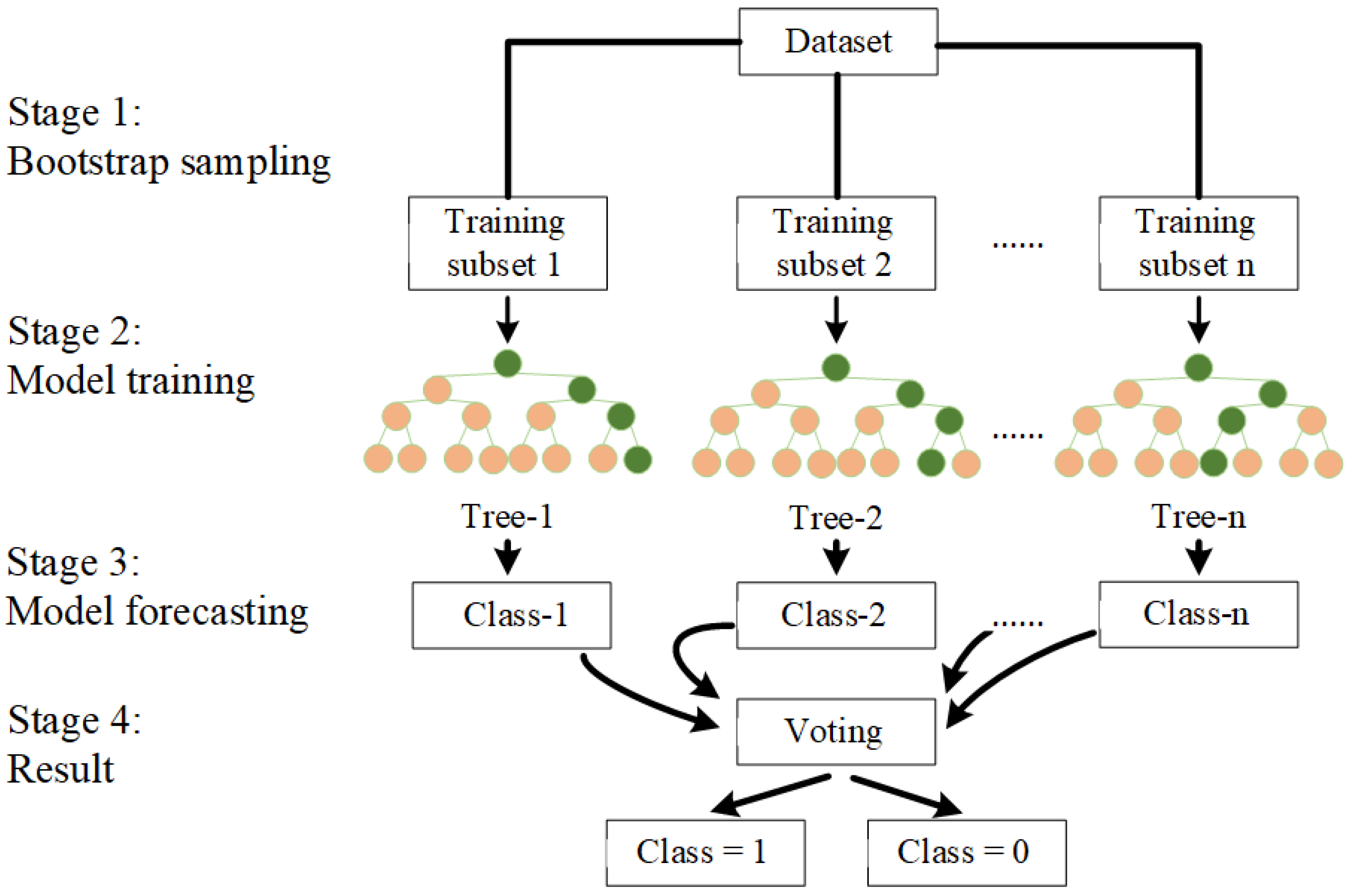
Random Forest (RF) is an ensemble learning method used for classification and regression tasks. It operates by training multiple decision trees and combining their results through a majority voting process for classification or averaging for regression tasks [36]. Each tree in the forest is trained on a subset of the original training data, and the final output category is determined by a majority vote among these trees, which is then converted into a corresponding classification probability [37]. A critical feature of the Random Forest algorithm is the random selection of a subset of variables for each node split, based on a specific metric. This approach enhances the model’s robustness and accuracy. Compared to other models, Random Forests consistently demonstrate the highest predictive accuracy in classification tasks [38] and are widely employed to handle datasets with a large number of predictors [39].
In the RF algorithm, parameters such as n estimators and max features significantly influence model performance. The n estimators parameter represents the number of decision trees in the ensemble. Increasing this value can enhance the model’s accuracy and generalization ability. The max features parameter denotes the number of candidate features randomly sampled each time a node is split. Two commonly used splitting criteria in Random Forests are Gini impurity and Information Gain [40]. Gini impurity measures the likelihood of incorrect classification of a randomly chosen element if it was randomly labeled according to the distribution of labels in the subset. The formula for Gini impurity is shown in Equation (4), which calculates the probability that two samples selected randomly from the set belong to different classes. Lower Gini impurity indicates higher purity of the subset. Information Gain is based on information entropy, which quantifies the reduction in uncertainty of the dataset after a split. Entropy measures the degree of disorder or chaos within a dataset, with higher entropy indicating more disorder. The formula for entropy is presented in Equation (5), while the formula for Information Gain is shown in Equation (6). Here, D represents the dataset, k is the number of classes, p i is the proportion of samples belonging to the i-th class, and D V is the subset of D where the feature A has value v.
Gini ( D ) = 1 i = 1 k p i 2
Entropy ( D ) = i = 1 k p i log 2 p i
Information   Gini ( D , A ) = Entropy ( D ) v Values ( A ) D v D Entropy D V
RF is an advanced decision tree model that enhances performance by incorporating additional randomness through the bagging method [41]. As illustrated in Figure 5, each decision tree within the RF ensemble serves as an individual prediction model, structured with nodes and edges. Decision trees contain two types of nodes: split (internal) nodes and leaf (terminal) nodes. Split nodes use a test function to partition the data based on different attributes, while leaf nodes correspond to the final decision result, such as a prediction or classification label. In the RF algorithm, each tree is trained on bootstrap samples (M samples) drawn from the total dataset. At each split node, only a randomly selected subset of features (max features) is considered, rather than all available features (N). This approach involves training M decision trees, and the final prediction is determined through average voting (for regression) or majority voting (for classification). The introduction of randomness serves to reduce the redundancy of explanatory variables and enhance the diversity of the individual decision trees within the ensemble, thereby improving the overall robustness and accuracy of the model [42].

3.2. Feature Importance

Random Forests use the bagging method to generate training sets, leaving approximately 1-1/N samples from the initial training set unselected. These unselected samples are known as out-of-bag (OOB) data. OOB samples are utilized not only for model training optimization but also for evaluating feature importance [43]. To determine feature importance, the reference score ( S r e f ) for a given feature X i is first calculated using the OOB sample. Then, the feature X i is randomly shuffled to obtain a new score ( S R S ). The importance score of the feature is calculated using Equation (7). This process is repeated for all features to generate an importance score for each one. The higher the score, the more important the feature is [44].
Importance X i = S r e f S R S

4. Training and Optimization of the WTCDA-RF Algorithm

When training a machine learning model, hyperparameters must be tuned and combined to optimize performance. For the RAndom Forest algorithm, commonly adjusted parameters include the split criterion (such as Entropy or Gini), the number of trees ( n _ e s t i m a t o r s ), and the size of the feature subset used for splitting ( m a x _ f e a t u r e s ). Manually tuning these hyperparameters is time consuming and challenging, so auxiliary algorithms are often employed for this task. One such method is the grid search algorithm (GSA), an exhaustive approach that explores all possible combinations of hyperparameters within a user specified range, determining the best combination through systematic training and evaluation [45].
Prior to training the Wind Turbine Clutter Classification Algorithm based on Random Forest (WTCDA-RF), the wind farm dataset is partitioned into a training set and a test set with an 8:2 ratio. The training set, comprising 7600 positive samples (class = 1) and 7600 negative samples (class = 0), is used for model optimization. The test set, consisting of 1900 positive samples (class = 1) and 1900 negative samples (class = 0), is used to evaluate model performance. Figure 5 illustrates the training and optimization process for the WTCDA-RF model.
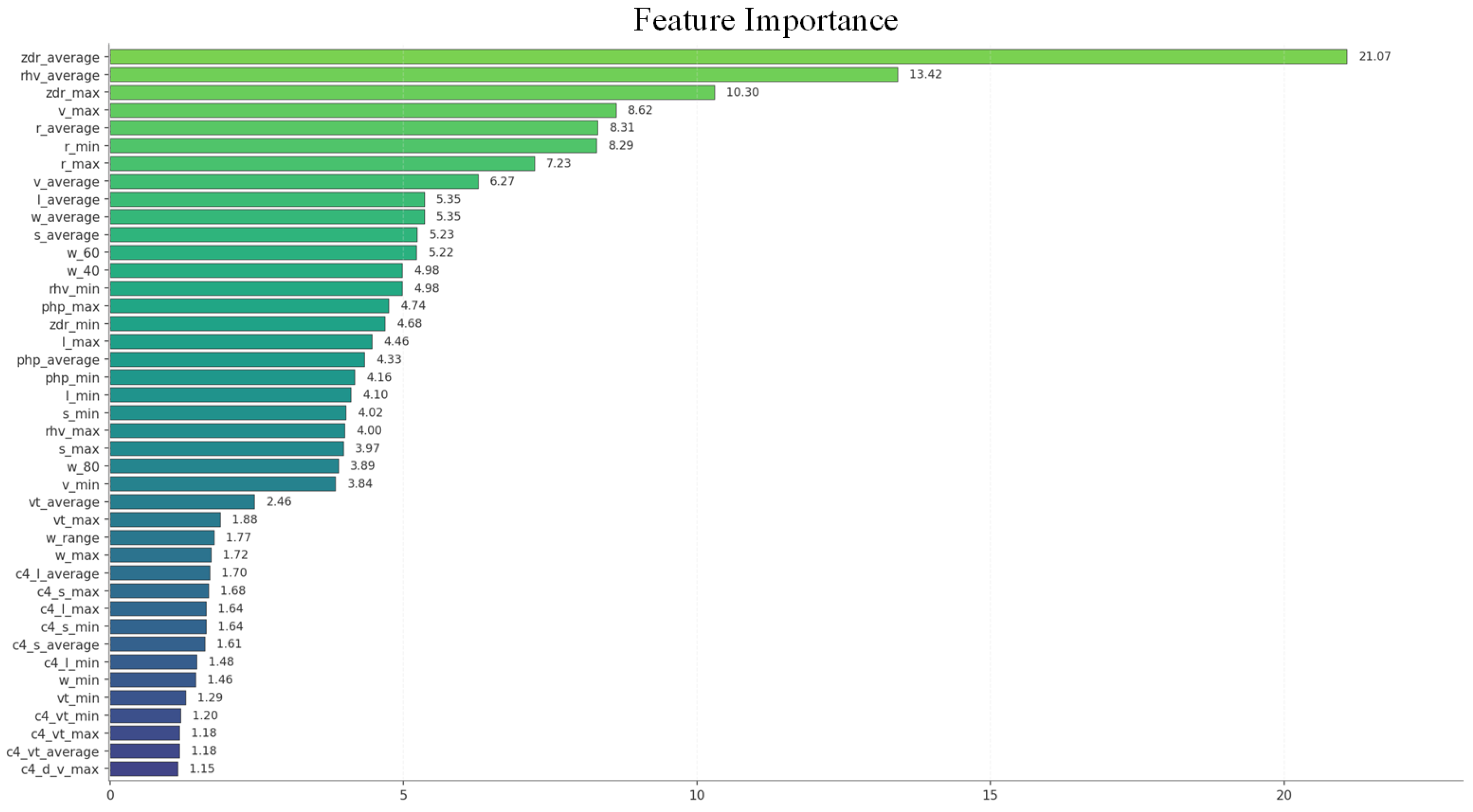
To enhance efficiency and reduce time consumption when employing grid search algorithms to explore a large number of parameter combinations, it is often necessary to conduct multiple iterations. In the initial search, the parameter range is broader with wider intervals, known as a rough search. Subsequent searches can leverage the outcomes of the initial search to further narrow the parameter range and reduce intervals for greater precision, which is referred to as fine-tuning. In Figure 6, the initial grid search produced a set of parameters: criterion: Gini, n _ e s t i m a t o r s : 230, and m a x _ f e a t u r e s : 9. Using these results as a reference, a more refined grid search was conducted, leading to a revised optimal combination: criterion: Entropy, n _ e s t i m a t o r s : 233, and m a x _ f e a t u r e s : 10. This refined search yielded the optimal model, labeled as Model-1 in Figure 6. This model represents the optimal configuration derived from training with a total of 41 features. The feature importance was then calculated using the corresponding module from the scikit-learn library, resulting in a ranked list of the 41 features, as depicted in Figure 7.
To maintain optimal model performance and speed, it is important to consider that an excessive number of features can adversely affect both model efficiency and, in some cases, classification accuracy. As a result, only the top 25 most important features are added in WTCDA-RF model, removing the remaining 16 less significant ones. In a Random Forest model, features ranked low in importance contribute least to the model’s predictive power. Such features will introduce noise, redundancy, or multicollinearity, potentially reducing model generalization. Therefore, after ranking all features by their mean decrease in impurity, only the top-ranked features that significantly improved classification performance were retained, while low-importance features were excluded to simplify the model and enhance robustness.
The WTCDA-RF model underwent retraining using a reduced set of 25 features. Hyperparameter optimization was conducted through two rounds of grid search to enhance the model’s performance. Initially, the hyperparameter set included criterion: Entropy, n _ e s t i m a t o r s : 110, and m a x _ f e a t u r e s : 7. After refinement, the updated set comprised criterion: Entropy, n _ e s t i m a t o r s : 109, and m a x _ f e a t u r e s : 6. This configuration represents the optimal WTCDA-RF model utilizing the 25 selected features, denoted as Model-2 in Figure 6. The evaluation results on the test set and the WTC recognition verification experiments in different regions will be used to verify the performance of the optimized WTCDA-RF algorithm.

5. Experimental Setup and Results

5.1. Evaluation of the WTCDA-RF Algorithm

In this study, we established a binary classification problem by categorizing samples into two groups, labeled class = 0 and class = 1. To evaluate the performance of the machine learning algorithm used for this binary classification, we utilized a confusion matrix [46]. The structure of this confusion matrix is illustrated in Table 2 below.
In the binary confusion matrix presented in Table 2, TP stands for “True Positives,” indicating the number of samples correctly predicted as positive by the model. FP refers to “False Positives,” representing the number of samples miss classified as positive. FN denotes “False Negatives,” indicating the number of samples incorrectly identified as negative, while TN, or “True Negatives,” represents the number of samples accurately classified as negative by the model. Given the two-class confusion matrix, we can derive several key metrics to evaluate the performance of the model, including accuracy (ACC), precision (PRE), F1-score, G-mean, probability of classification (POD), false alarm rate (FAR), and critical success index (CSI). These metrics are defined by the following formulas:
  • ACC (Equation (8)) represents the proportion of correct predictions within the overall dataset, reflecting the model’s overall accuracy.
  • PRE (Equation (9)) indicates the precision of the model, measuring its accuracy in identifying positive samples.
  • The F1-score (Equation (10)) is a harmonic mean of precision and recall (with Recall = TP/ (TP + FN)), offering a balanced measure of the model’s accuracy and completeness.
  • G-mean (Equation (11)) is used to evaluate models with class imbalance and reflect show balanced the model is. A higher G-mean indicates better balance.
  • POD (Equation (12)) denotes the model’s hit rate, indicating the proportion of true positives among actual positives.
  • FAR (Equation (13)) represents the false alarm rate, indicating the proportion of false positives among predicted positives.
  • CSI (Equation (14)) stands for the critical success index, providing an overall measure of the model’s performance.
A C C = T P + F N P C + N C
P R E = T P T P + F P
F 1 -score = 2 × recall × P R E recall + P R E
G -mean = T P T P + F N × T N T N + F P
P O D = T P T P + F N
F A R = F P T P + F P
C S I = T P T P + F N + F P
These metrics, taken together, offer a comprehensive view of the model’s effectiveness in predicting wind turbine clutter. Each plays a distinct role in assessing the model’s accuracy, precision, balance, and reliability [47].
After identifying the optimal parameters for the WTCDA-RF model, we constructed a wind turbine clutter identification model using these parameters. The test set was then input into this model to evaluate its performance. The specific scores calculated from a series of relevant indicators are presented in Table 3. High accuracy and precision indicate that the model performs well overall, with a low rate of false positives in positive predictions. A high F1-score suggests that the model maintains a balanced approach between false positives and false negatives. A high recall rate signifies that the model successfully captures the majority of positive instances. Probability of classification (POD) and false alarm rate (FAR) are significant metrics for risk assessment. A high POD coupled with a low FAR implies that the model accurately identifies most positive examples while minimizing false alarms. The critical success index (CSI) combines the effects of both false positives and false negatives. A high CSI score demonstrates that the model excels at accurately predicting positive instances.
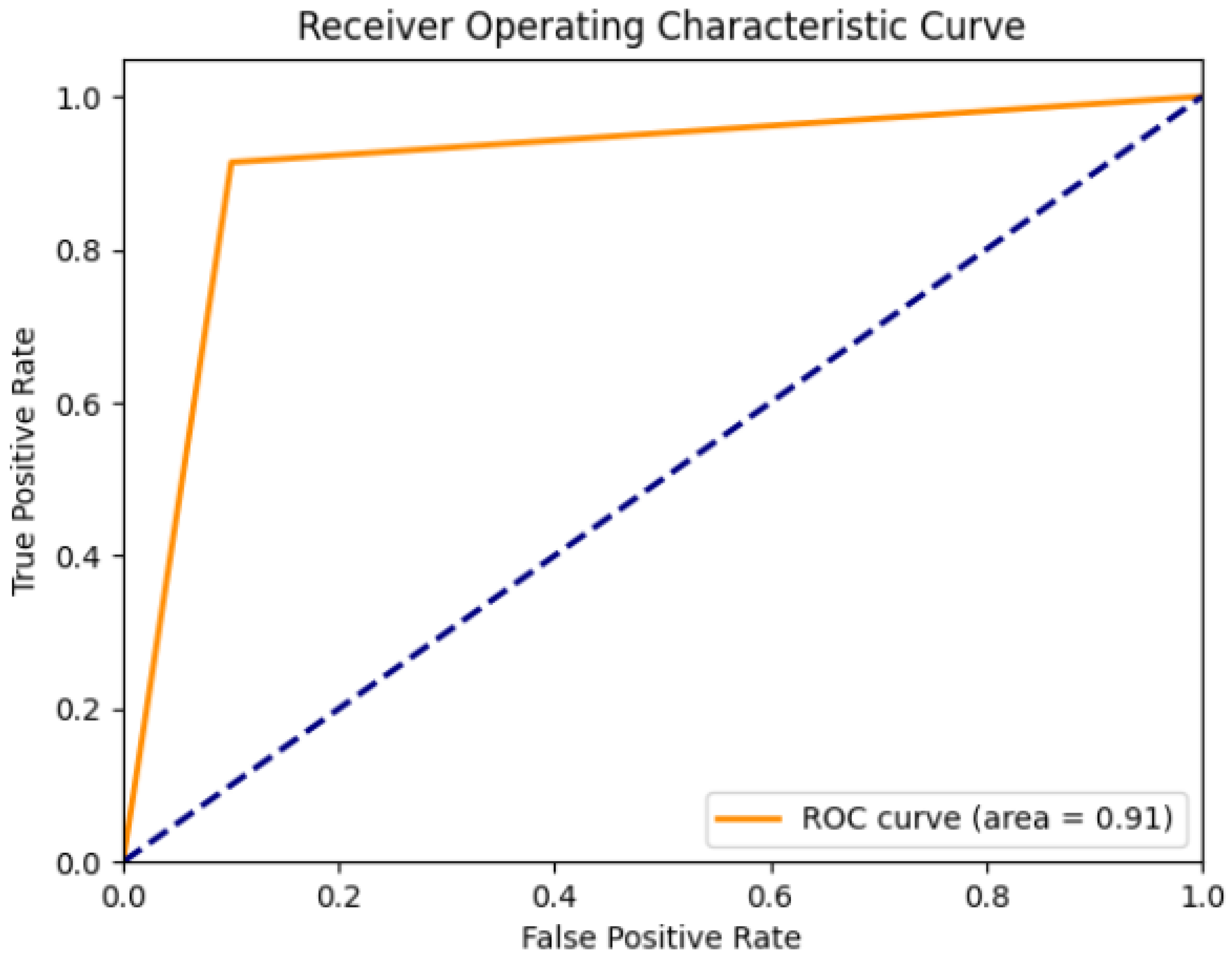
This study further presents the Receiver Operating Characteristic (ROC) curve, as illustrated in Figure 8, to evaluate the classification performance of the WTCDA-RF model. The ROC curve characterizes the trade-off between the true positive rate and the false positive rate, where a curve closer to the upper-left corner reflects stronger discriminative capability. The Area Under the Curve (AUC) is a widely adopted quantitative metric for classification performance, with values ranging from 0 to 1, and values closer to 1 indicating superior performance. Experimental results demonstrate that the AUC for both positive and negative categories is identical, at 0.9108, suggesting that the model exhibits balanced discriminative ability between wind farm clutter and non-wind farm clutter. The absence of a significant bias toward either class indicates stable prediction performance. Furthermore, the AUC value of 0.91 and the ROC curve’s proximity to the upper-left corner collectively confirm the strong classification capability of the proposed model.

5.2. Detection of Wind Turbine Clutter Using the WTCDA-RF Algorithm

The performance of the WTCDA-RF model was evaluated by conducting WTC detection experiments under different weather conditions in Nantong and WTC in other regions of China to assess the accuracy of the algorithm and its cross-regional detection capabilities.
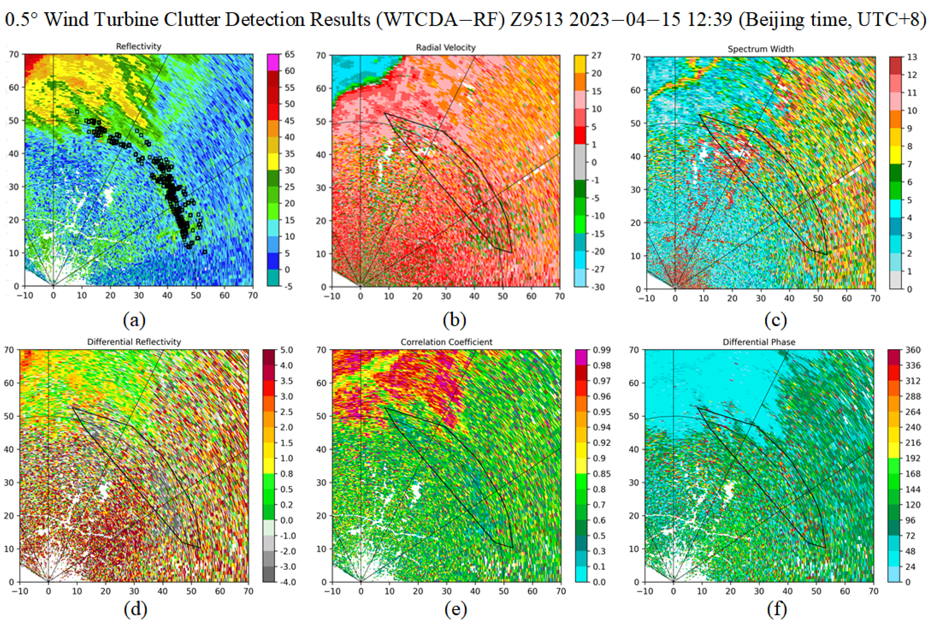
The performance of the WTCDA-RF model was evaluated through a wind turbine clutter classification study conducted in Nantong, Jiangsu Province. The wind farm, located approximately 32 miles (about 51 km) from the radar, was determined using Google Maps (refer to Figure 9). The wind turbine clutter recognition probability threshold is set to be greater than 0.6 to verify the effectiveness of the algorithm under different weather conditions. For blocks whose identification probability meets the threshold, the WTC classification hit rate is calculated, which is the proportion falling within the wind farm area. The identification results of the WTCDA-RF model are marked with small black rectangles in the reflectivity echo map. The radial velocity, spectral width, differential reflectivity, correlation coefficient and differential phase shift are also shown in the results. The significant WTC polarization characteristics can be seen by comparing the area.
From 10:39 to 18:51 Beijing time on 15 April 2023, basic radar data was collected from the Nantong radar station during six distinct weather conditions. Utilizing a pre-trained Random Forest model, features were extracted from the radar data and predictions were made on the secondary radar data. By correlating the prediction outcomes with relevant location data, the distribution of radar data with varying characteristics was visualized. This facilitated the depiction of offshore wind turbine clutter classification results as predicted by the Random Forest model.
Figure 10 illustrates a PPI under no-precipitation weather conditions. The impact of WTC on all radar parameters is visible through the 50 km radial distance ring. At an elevation angle of 0.5°, the reflectivity values hover around 30 dBZ, while the differential reflectivity (ZDR) registers slightly negative values near the 50 km radial distance mark. The observed velocities fluctuate between negative and positive values. The observed speed fluctuates between positive and negative values. It can be seen that the WTC and weather process echoes are superimposed in the radar data, which interferes with the identification of the weather process and makes it difficult to accurately predict the evolution of the weather process.
Figure 11 depicts radar parameter diagrams under different precipitation conditions. The impact of wind turbine clutter on all radar parameters within the 50 km radial range is evident. Compared to reflectivity measurements in no-precipitation conditions, the reflectivity values in these scenarios are quite similar, generally ranging from 10 to 35 dBZ. In cases of heavier precipitation, reflectivity in small localized areas can reach up to 50 dBZ. Wind turbines, due to their blocky and tall structures, cause the vertically polarized reflectivity ( Z V ) to be higher than the horizontally polarized reflectivity ( Z H ), leading to negative differential reflectivity (ZDR) within wind turbine clutter areas. The rotation of the wind turbine blades contributes to higher radial velocity measurements in cluttered areas compared to the actual wind speed. Under precipitation conditions, the wind turbines have little influence on differential phase shift ( Φ DP ) readings. The correlation coefficient (CC) measurements within the cluttered areas vary from 0.6 to 0.8.
The evaluation of the WTCDA-RF model in Table 4, combined with six independent cases outside the dataset of Nantong Z9513 radar, demonstrates the model’s reliable performance in identifying WTC under various meteorological conditions. These case studies further confirm that, when combined with dual-polarization radar data, the model can effectively capture clutter characteristics and maintain high detection accuracy in practical applications.
In the experiment, we observed significant areas of clutter interference at approximately 0.7 km and 2.5 km, both upstream and downstream of the wind farm. During precipitation events, the clutter interference areas tended to be more extensive. The identification outcomes differ notably under clear sky and precipitation weather conditions. One plausible explanation for these disparities lies in variations in the “angle of attack” of wind turbine blades. The angle of attack refers to the angle at which individual blades are vertically inclined concerning the average airflow to generate optimal lift. It is essential to clarify that, within this context, the angle of attack is not a meteorological concept but rather a hydrodynamic one employed by wind energy firms to maximize energy output from a wind farm under specific wind scenarios. Another potential explanation pertains to the operational status of wind turbines. Uncertainty prevails regarding whether the wind turbine is currently operational, which could also contribute to the disparity in results.
The Random Forest (RF)-based wind turbine clutter classification and identification method introduced in this study demonstrated robust applicability under various meteorological conditions. Under precipitation conditions, certain features may lead to misclassification and misidentification of clutter. However, prior to training the RF model, our method selects and filters features to retain the most discriminative and relevant ones. This approach enhances the model’s ability to differentiate between actual weather targets and clutter, thus improving classification accuracy. The Random Forest-based wind turbine clutter classification method proposed in this study has demonstrated effectiveness in detecting and identifying wind turbine clutter even under special meteorological conditions.
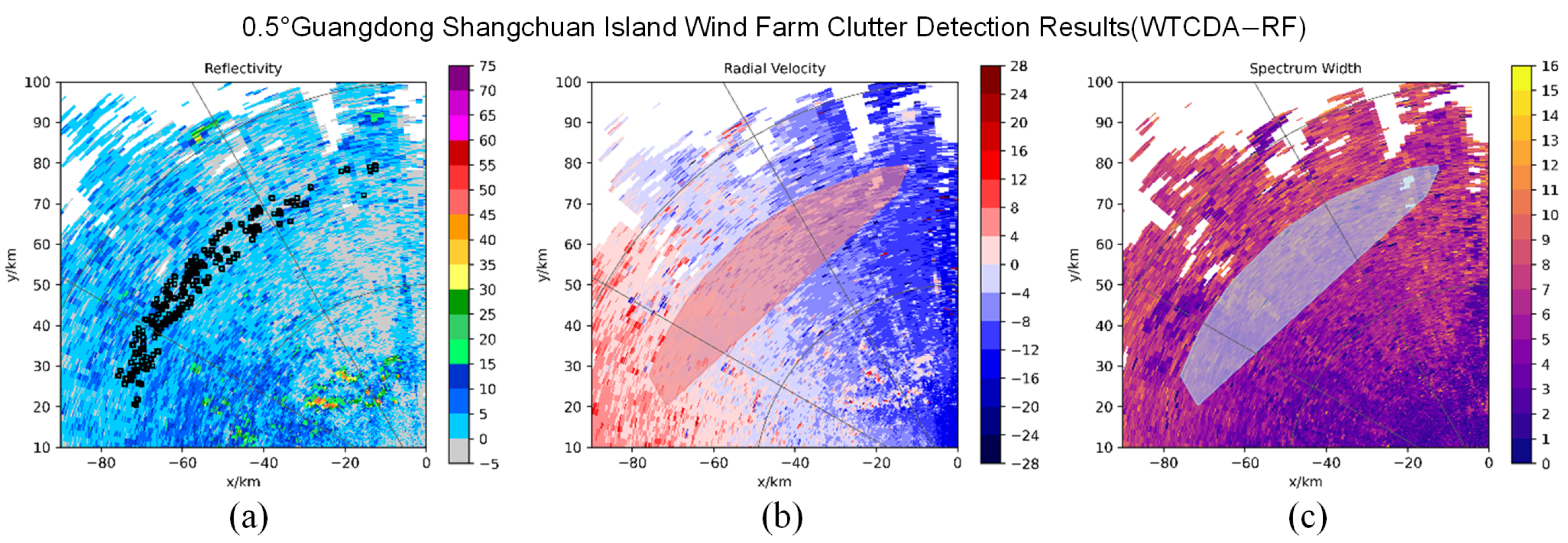
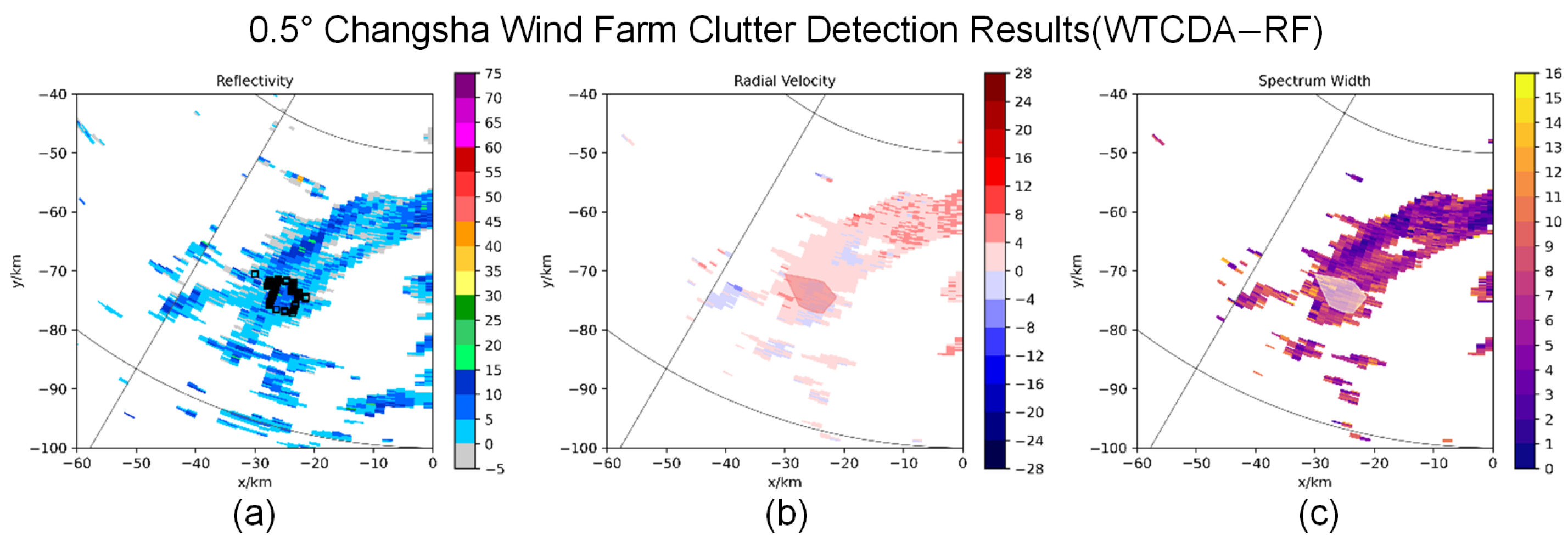
The WTCDA-RF model was applied to detect WTCs at other locations to verify the versatility of the algorithm, after training with the Nantong WTC dataset. Figure 12, Figure 13 and Figure 14 illustrate the clutter classification results of wind turbines and wind turbines obtained using the WTCDA-RF algorithm at the Shangchuan Island radar in Guangdong Province, Changsha radar in Hunan Province, and Yantai radar in Shangdong Province. Comparing the geographical location with the actual wind farm, we found a high degree of consistency between the identified clutter areas and the location of the wind farm. This suggests that the proposed algorithm successfully identifies clutter areas with a high degree of accuracy, providing reliable results when applied to radar data.
The WTCDA-RF, the fuzzy logic-based WTC detection algorithm (WTCDA-FL) proposed by [28], and a Convolutional Neural Network-based WTC detection algorithm (WTCDA-CNN) were compared and tested using WTC data from Changsha, Shangchuan Island, and Yantai that were not included in the training set. The test results are summarized in Table 5. WTCDA-RF achieved the highest POD and CSI values with the lowest FAR, demonstrating superior detection capability and generalization performance. WTCDA-CNN outperformed WTCDA-FL in all three metrics, highlighting the potential of deep learning for WTC detection, though it still lagged behind WTCDA-RF in robustness and accuracy. The WTCDA-FL algorithm relies mainly on WTC thresholds in various radar products calculated from Yantai radar data, making it sensitive to weather conditions and geographical differences and difficult to generalize to other regions. For the deep learning model WTCDA-CNN, given the limited size of the available dataset, its performance may not yet reflect its full potential; we believe that with a substantially larger and more diverse training dataset, its detection accuracy and robustness could be further improved. In contrast, the WTCDA-RF algorithm can mitigate the influence of weather conditions on detection results, enabling better adaptability across diverse scenarios.

6. Discussion

In the “feature importance ranking” approach, among the top 25 fundamental features (with importance scores exceeding 2.18), attributes associated with the differential reflectivity (ZDR) constitute a significant portion. This underscores the high sensitivity of ZDR to wind farm presence. ZDR characterizes the average particle shape within the classification volume (range cell), and its mathematical expression is as follows:
Z D R = 10 × log 10 Z H Z V
where Z H and Z V denote the radar reflectivity factors in the horizontal and vertical polarizations, respectively. When horizontal energy dominates ( Z H > Z V ), ZDR > 0 dB; conversely, when vertical energy dominates, ZDR < 0 dB. Spherical particles or randomly oriented non-spherical particles scatter energy equally in both polarizations, yielding ZDR ≈ 0 dB. ZDR is derived from filtered moments of static ground clutter, with wind farm echoes typically exhibiting distinctly negative values (−4 to −1 dB). This characteristic persists and serves as a reliable discriminator between wind farm echoes and meteorological echoes. Moreover, wind farm structures exhibit strong directional properties, producing anisotropic reflectivity that induces noticeable variations in differential reflectivity. These variations often appear as striped or patchy patterns on ZDR maps. Since wind turbine blades and other structural components possess scattering properties different from natural hydrometeors (e.g., raindrops, snowflakes), they frequently cause abnormal fluctuations in ZDR, deviating from typical meteorological values. Such anomalous ZDR signatures therefore provide a key indicator of wind farm clutter.
Reflectivity factors play a pivotal role in wind turbine clutter classification. Analysis of classification results reveals that reflectivity factor values associated with wind turbine clutter tend to be notably elevated, typically ranging from 10 to 35 dBZ on average. In certain regions, isolated areas exhibit reflectivity values surpassing 50 dBZ, indicating a non-uniform spatial distribution. Wind farm structures, including wind turbines and turbine blades, scatter radar waves, resulting in fluctuations in reflectivity. These structures, characterized by intricate geometries and diverse surface properties, typically yield higher reflectivity factors. Furthermore, other obstacles within the radar’s field of view, such as nearby highrise buildings, may also contribute to heightened average reflectivity levels. Moreover, meteorological conditions, such as atmospheric humidity and temperature, may exert influence on the reflectivity factor of wind turbine clutter. For instance, increased humidity can lead to water droplet condensation on target surfaces, intensifying radar wave scattering and consequently augmenting the reflectivity factor.
Wind turbine clutter exerts a distinctive influence on radial velocity and holds significant importance in terms of feature relevance. This clutter induces Doppler shifts in the observed radial velocity due to the motion of wind turbine blades relative to the radar, consequently altering the frequency of the received echo signal. This Doppler shift serves as a crucial indicator for detecting and distinguishing wind turbine clutter. Within wind farms, the rotational movement of wind turbine blades is typically evident in the radial velocity data obtained from weather radar. Therefore, discerning and accurately interpreting this rotational effect is imperative for precise analysis of radial velocity data and for ensuring the accuracy of weather observations.
Within the realm of wind turbine clutter analysis, the correlation coefficient emerges as a pivotal metric for assessing radar signal coherence. Typically denoted as ρ HV or CC, this coefficient quantifies the correlation between changes in amplitude and phase of radar pulses polarized horizontally and vertically. It provides insights into the consistency of particle shape and orientation within the radar beam. Spherical particles or those with minimal shape and orientation variability typically yield high correlation coefficients. In meteorological contexts, precipitation targets like rain or snow often exhibit correlation coefficients surpassing 0.8, indicating strong agreement between horizontal and vertical polarization echoes. However, structural elements such as rotating turbines and towers within wind farms can introduce instability or irregular fluctuations in correlation coefficient data. The distinct reflectivity and phase characteristics of structural targets compared to natural meteorological entities (e.g., raindrops or snowflakes) result in notable reductions in the correlation coefficient. The rotational motion of wind turbines generates erratic reflection patterns, contributing to fluctuations in the correlation coefficient and indicating diminished signal coherence compared to natural weather phenomena. Thus, diligent examination of correlation coefficient data for discontinuities or abnormal fluctuations is essential, as they may signify the presence of wind farm clutter. A comprehensive analysis of correlation coefficient data can refine weather forecasts and fortify the dependability of radar observations.
For wind farm clutter, the differential propagation phase shift ( Φ DP ) exhibits distinctive characteristics, as it represents the polarization phase difference accumulated along the radial direction within one radar pulse cycle ( Φ DP = Φ HH Φ VV ). Since direct analysis of Φ DP is often challenging, its derivative, the specific differential phase (KDP), is typically employed to describe the rate of change of phase difference. This phase shift arises due to the inherent phase difference between horizontally and vertically polarized waves as they traverse through precipitation. Non-spherical particles are the primary cause of this phase disparity: particles with greater mass distributed horizontally yield KDP > 0°/km, whereas those with greater mass distributed vertically yield KDP < 0°/km. There exists a correlation between differential propagation phase shift and reflectivity, particularly for materials like ice crystals. Wind farm clutter typically stems from structural targets, and the reflectivity–phase relationship may differ from natural meteorological targets (e.g., raindrops, snowflakes, etc.). Therefore, it is essential to consider this unique relationship between reflectivity and phase when interpreting differential phase shift rate data. Wind farm clutter induces phase discontinuities or abnormal variations in differential propagation phase shift data. These anomalies result from phase alterations caused by structural targets. Hence, during the analysis and identification of wind farm clutter, detecting and analyzing such phase discontinuities and abnormal variations is imperative.
Experiments have demonstrated that the WTCDA-RF algorithm is effective in identifying clutter distribution caused by wind farms in weather radar observations, providing a robust method for the subsequent elimination of wind turbine clutter. In future research, this algorithm will be employed to eliminate wind turbine clutter areas and to reconstruct low-level elevation data using radar high-level elevation data, as wind turbine clutter mainly affects the radar’s 0.5° and 1.5° elevation data.

7. Conclusions

This paper presents a Wind Turbine Clutter Classification Algorithm based on a Random Forest approach, designed for use with the CINRAD-SAD radar system to identify wind turbine clutter. The algorithm processes radar level-II data, including reflectivity, radial velocity, and velocity spectrum width, as well as differential reflectivity, differential phase shift rate, and correlation coefficient. The method begins by segmenting the radar data into blocks and calculating relevant features. The wind farm dataset is then labeled according to the geographic location of the wind farm. Subsequently, a Random Forest-based wind turbine clutter classification algorithm (WTCDA-RF) is developed. The following key conclusions were reached:
  • Differential reflectivity-related features play a crucial role in wind turbine clutter classification. By incorporating the differential phase shift rate from weather radar data and combining it with radial velocity-related features, the classification and identification of wind turbine clutter can be further enhanced.
  • The echo characteristics of wind turbine clutter have been analyzed, revealing features such as strong reflectivity, rapid changes in radial velocity, and a large spectral width. Notably, wind turbine clutter (WTC) signals can sometimes resemble weather signals in terms of power and spectral content, complicating their differentiation on Planar Position Indicator (PPI) weather radar images. In contrast, ground clutter primarily arises from radar wave reflections off the ground and nearby objects. Its distribution tends to be broader, with more complex reflectivity characteristics, and is heavily influenced by terrain and surrounding ground-based structures.
  • The WTCDA-RF algorithm leverages intra-block features and employs a Random Forest classification approach to address a range of influencing factors. By combining multiple sets of level-II radar echo data, it effectively detects and identifies wind turbine clutter near the radar, achieving comprehensive wind power interference identification. The WTCDA-RF algorithm demonstrates high accuracy and precision, alongside a low false alarm rate, indicating its robust applicability in wind turbine clutter recognition tasks.
Future research directions include the following:
  • Deep learning methods offer notable advantages for handling wind turbine clutter. These models are adept at learning complex nonlinear patterns and extracting relevant feature information from large datasets automatically. Moreover, deep learning techniques support end-to-end learning, allowing the model to process raw data directly and produce predictions or classifications without manual feature extraction. This capability minimizes manual intervention and reduces subjective bias, resulting in greater accuracy and efficiency in data processing.
  • The structural characteristics of wind turbines also play a crucial role in their impact on radar observations. For instance, recent studies on inflatable Savonius wind turbines with rapid deployment and retrieval capability [48] indicate that innovative designs can not only enhance wind energy utilization efficiency but also potentially reduce radar cross section (RCS) and clutter interference. Therefore, future research should consider a combined perspective of both advanced clutter detection algorithms and structural optimization of wind turbines to further improve the quality of Doppler weather radar data.
  • Expanding the dataset to include weather radar affected by both offshore and onshore wind parks will be a key step toward improving the model’s robustness and generalization. Such diverse data sources will enable the model to learn a broader range of WTC characteristics, thereby enhancing its detection capability under varying geographical and meteorological conditions.

Author Contributions

Conceptualization, F.Z., Y.G., Q.Z., H.W. and Z.R.; methodology, F.Z., Y.G., Q.Z. and Z.R.; software, Y.G., Z.R., Q.Z. and F.Z.; validation, F.Z., Q.Z. and Z.R.; formalanalysis, F.Z., Q.Z., H.W. and Z.R.; investigation, F.Z.; resources, Q.Z. and H.W.; data curation, F.Z. writing—original draft preparation, F.Z. and Y.G.; writing review and editing, Q.Z., H.W. and Z.R.; visualization, Y.G. and Q.Z.; supervision, Q.Z., H.W., Z.R. and W.C.; project administration, Q.Z. and H.W.; funding acquisition, Q.Z. All authors have read and agreed to the published version of the manuscript.

Funding

This research was funded by the National Natural Science Foundation of China (U2342216), China Meteorological Administration Tornado Key Laboratory (Grant TKL202309), China Meteorological Administration projects (CMAJBGS202316), Key Laboratory of Strait Disaster Weather (2022K04), the Joint Research Project for Meteorological Capacity Improvement (22NLTSY009); the fund of “Key Laboratory of Atmosphere Sounding, CMA” (2021KLAS01M); the Innovation and Development Project of China Meteorological Administration (CXFZ2023J022).

Data Availability Statement

The original contributions presented in the study are included in the article; further inquiries can be directed to the corresponding author.

Acknowledgments

The authors are grateful for the use of S-band radar data from Jiangsu Detection Center. The authors are also grateful to the researchers whose published papers contain information used and cited in this paper.

Conflicts of Interest

The authors declare no conflicts of interest.

Abbreviations

The following abbreviations are used in this manuscript:
WTCWind Turbine Clutter
PPIPlan Position Indicator
I/Qin-phase and quadrature-phase
FISFuzzy Inference System
RFRandom Forest
OOBOut-of-Bag
QPEQuantitative estimation of precipitation
GSAGrid Search Algorithm

Appendix A

Table A1. The 40 features and their explanations, with the critical 25 features bolded. Note: Features prefixed with “c4” are derived from calculations based on the central 2 × 2 region within the 4 × 4 grid.
FeatureImplicationUnit
r_averagethe average value in the 4 × 4 reflectivit blockdBZ
r_maxthe maximum value in the 4 × 4 reflectivit blockdBZ
r_minthe minimum value in the 4 × 4 reflectivit blockdBZ
v_averagethe average value in the 4 × 4 velocity blockm/s
v_maxthe maximum value in the 4 × 4 velocity blockm/s
v_minthe minimum value in the 4 × 4 velocity blockm/s
w_averagethe average value in the 4 × 4 spectrum width blockm/s
w_maxthe maximum value in the 4 × 4 spectrum width blockm/s
w_minthe minimum value in the 4 × 4 spectrum width blockm/s
zdr_averagethe average value in the 4 × 4 differential reflectivity blockdB
zdr_maxthe maximum value in the 4 × 4 differential reflectivity blockdB
zdr_minthe minimum value in the 4 × 4 differential reflectivity blockdB
php_averagethe average value in the 4 × 4 differential phase block°
php_maxthe maximum value in the 4 × 4 differential phase block°
php_minthe minimum value in the 4 × 4 differential phase block°
rhv_averagethe average value in the 4 × 4 correlation coefficient block
rhv_maxthe maximum value in the 4 × 4 correlation coefficient block
rhv_minthe minimum value in the 4 × 4 correlation coefficient block
s_averagethe average value of velocity difference in the 4 × 4 V blockm/s
s_maxthe maximum value of velocity difference in the 4 × 4 V blockm/s
s_minthe minimum value of velocity difference in the 4 × 4 V blockm/s
l_averagethe average value of horizontal wind sheer in the 4 × 4 V blocks−1
l_maxthe maximum value of horizontal wind sheer in the 4 × 4 V blocks−1
l_minthe minimum value of horizontal wind sheer in the 4 × 4 V blocks−1
vt_averagethe average value of horizontal wind direction gradient in the 4 × 4 V block°/m
vt_maxthe maximum value of horizontal wind direction gradient in the 4 × 4 V block°/m
vt_minthe minimum value of horizontal wind direction gradient in the 4 × 4 V block°/m
c4_s_averagethe average value of velocity difference in the 2 × 2 V blockm/s
c4_s_maxthe maximum value of velocity difference in the 2 × 2 V blockm/s
c4_s_minthe minimum value of velocity difference in the 2 × 2 V blockm/s
c4_l_averagethe average value of horizontal wind sheer in the 2 × 2 V blocks−1
c4_l_maxthe maximum value of horizontal wind sheer in the 2 × 2 V blocks−1
c4_l_minthe minimum value of horizontal wind sheer in the 2 × 2 V blocks−1
c4_vt_averagethe average value of horizontal wind direction gradient in the 2 × 2 V block/m
c4_vt_maxthe maximum value of horizontal wind direction gradient in the 2 × 2 V block/m
c4_vt_minthe minimum value of horizontal wind direction gradient in the 2 × 2 V block/m
w_rangethe range value of velocity spectral width in the 4 × 4 W blockm/s
w_40the threshold greater than 40% velocity spectral width in the 4 × 4 W blockm/s
w_60the threshold greater than 60% velocity spectral width in the 4 × 4 W blockm/s
w_80the threshold greater than 80% velocity spectral width in the 4 × 4 W blockm/s

References

  1. Liu, Y.; Zeng, Z.T. Wind Energy; Springer International Publishing: Cham, Switzerland, 2023; pp. 129–145. [Google Scholar] [CrossRef]
  2. Jiang, Q.; Yin, Z. The optimal path for China to achieve the “dual carbon” target from the perspective of energy structure optimization. Sustainability 2023, 15, 10305. [Google Scholar] [CrossRef]
  3. Lee, J.; Zhao, F. Gwec Global Wind Report 2024; Global Wind Energy Council: Brussels, Belgium, 2024. [Google Scholar]
  4. Ritschel, U.; Beyer, M. Modern Wind Turbines; Springer International Publishing: Cham, Switzerland, 2022; pp. 13–41. [Google Scholar] [CrossRef]
  5. Burgess, D.W.; Crum, T.; Vogt, R. Impacts of wind farms on wsr-88d radars. In Proceedings of the 24th International Conference on Interactive Information and Processing Systems for Meteorology, Oceanography, and Hydrology, New Orleans, LA, USA, 20–24 January 2008. [Google Scholar]
  6. Isom, B.; Palmer, R.; Secrest, G.; Rhoton, R.D.; Saxion, D.; Allmon, T.L.; Reed, J.; Crum, T.; Vogt, R. Detailed observations of wind turbine clutter with scanning weather radars. J. Atmos. Ocean. Technol. 2009, 26, 894–910. [Google Scholar] [CrossRef]
  7. Theil, A.; Schouten, M.W.; de Jong, A. Radar and wind turbines: A guide to acceptance criteria. In Proceedings of the 2010 IEEE Radar Conference, Arlington, VA, USA, 10–14 May 2010; pp. 1335–1341. [Google Scholar] [CrossRef]
  8. Chandra, M.; Gekat, F. Interference in weather radars caused by windparks: Scattering model for weather radar signal processing. In Proceedings of the 12th European Conference on Antennas and Propagation (EuCAP 2018), London, UK, 9–13 April 2018; pp. 1–4. [Google Scholar] [CrossRef]
  9. Sergey, L.; Hubbard, O.; Ding, Z. Advanced mitigating techniques to remove the effects of wind turbines and wind farms on primary surveillance radars. In Proceedings of the 2008 IEEE Radar Conference, Rome, Italy, 26–30 May 2008; pp. 1–6. [Google Scholar] [CrossRef]
  10. Hubbert, J.; Dixon, M.; Ellis, S. Weather radar ground clutter. Part II: Real-time identification and filtering. J. Atmos. Ocean. Technol. 2009, 26, 1181–1197. [Google Scholar] [CrossRef]
  11. Vogt, R.J.; Crum, T.; Snow, J.T.; Palmer, R.D.; Isom, B.; Burgess, D.Q.; Paese, M.S. An update on policy considerations of wind farm impacts on WSR-88D operations. In Proceedings of the 24th International Conference on Interactive Information Processing Systems (IIPS) for Meteorology, Oceanography, and Hydrology, New Orleans, LA, USA, 20–24 January 2008; pp. 1–11. [Google Scholar]
  12. Vogt, R.J.; Reed, J.; Crum, T. Impacts of wind farms on wsr-88d operations and policy considerations. In Proceedings of the 23rd International Conference on Interactive Information Processing Systems (IIPS) for Meteorology, Oceanography, and Hydrology, San Antonio, TX, USA, 15–18 January 2007; pp. 141–147. [Google Scholar]
  13. Droegemeier, K.K. The advanced regional prediction system (arps), storm-scale numerical weather prediction and data assimilation. Meteorol. Atmos. Phys. 2003, 82, 139–170. [Google Scholar] [CrossRef]
  14. Carpenter, T.M.; Georgakakos, K.P.; Sperfslagea, J.A. On the parametric and nexrad-radar sensitivities of a distributed hydrologic model suitable for operational use. J. Hydrol. 2001, 253, 169–193. [Google Scholar] [CrossRef]
  15. Rossa, A.; Liechti, K.; Zappa, M. The cost 731 action: A review on uncertainty propagation in advanced hydro-meteorological forecast systems. Atmos. Res. 2011, 100, 150–167. [Google Scholar] [CrossRef]
  16. Crum, T.; Ciardi, E. Wind farms and the wsr-88d: An update. Nexrad Now 2010, 19, 17–22. [Google Scholar]
  17. Vogt, R.J.; Crum, T.D.; Greenwood, W. New criteria for evaluating wind turbine impacts on nexrad weather radars. In Proceedings of the WINDPOWER 2011, Anaheim, CA, USA, 22–25 May 2011; Volume 4, pp. 13–17. [Google Scholar]
  18. Toth, M.; Jones, E.; Pittman, D. Dow radar observations of wind farms. Bull. Am. Meteorol. Soc. 2011, 92, 987–995. [Google Scholar] [CrossRef]
  19. Norin, L.; Haase, G. Doppler weather radars and wind turbines. In Doppler Radar Observations-Weather Radar, Wind Profiler, Ionospheric Radar, and Other Advanced Applications; INTECH Open Access Publisher: London, UK, 2012; Volume 53, pp. 323–327. [Google Scholar]
  20. Norin, L. A quantitative analysis of the impact of wind turbines on operational doppler weather radar data. Atmos. Meas. Tech. 2015, 8, 593–609. [Google Scholar] [CrossRef]
  21. Gallardo-Hernando, B.; Perez-Martinez, F.; Aguado-Encabo, F. Wind turbine clutter detection in scanning weather radar tasks. In Proceedings of the 6th European Conference on Radar in Meteorology and Hydrology, Sibiu, Romania, 6–10 September 2010; Volume 63, pp. 772–778. [Google Scholar]
  22. Nai, F.; Torres, S.; Palmer, R. On the mitigation of wind turbine clutter for weather radars using range-doppler spectral processing. IET Radar Sonar Navig. 2013, 7, 178–190. [Google Scholar] [CrossRef]
  23. Hood, K.; Torres, S. Automatic detection of wind turbine clutter for weather radars. J. Atmos. Ocean. Technol. 2010, 27, 1868–1880. [Google Scholar] [CrossRef]
  24. Cheong, B.L.; Palmer, R.; Torres, S. Automatic wind turbine identification using level-II data. In Proceedings of the 2011 IEEE RadarCon (RADAR), Kansas City, MO, USA, 23–27 May 2011. [Google Scholar] [CrossRef]
  25. Seo, B.C.; Krajewski, W.F. Using the new dual-polarimetric capability of wsr-88d to eliminate anomalous propagation and wind turbine effects in radar-rainfall. Atmos. Res. 2015, 153, 296–309. [Google Scholar] [CrossRef]
  26. He, W.; Wu, R.; Wang, X. Meteorological radar wind farm clutter detection and identification method based on level-II data and fuzzy logic reasoning. J. Electron. Inf. Technol. 2017, 39, 1748–1758. [Google Scholar] [CrossRef]
  27. Norin, L. Wind turbine impact on operational weather radar i/q data: Characterisation and filtering. Atmos. Meas. Tech. 2017, 10, 1739–1753. [Google Scholar] [CrossRef]
  28. Su, T.; Ge, J. Wind turbine clutter identification and suppression for cinrad. J. Mar. Meteorol. 2023, 43, 45–58. [Google Scholar] [CrossRef]
  29. Wang, Z.; Chen, H.; Yuan, S. New generation dual-polarization weather radar (cinrad/sad) refined detection technology. Meteorol. Sci. Technol. 2020, 48, 331–336. [Google Scholar]
  30. Chandrasekar, V.; Kernen, R.; Lim, S. Recent advances in classification of observations from dual polarization weather radars. Atmos. Res. 2013, 119, 97–111. [Google Scholar] [CrossRef]
  31. Bluestein, H.B.; Rauber, R.M.; Burgess, D.W. Radar in atmospheric sciences and related research: Current systems, emerging technology, and future needs. Bull. Am. Meteorol. Soc. 2014, 95, 1850–1861. [Google Scholar] [CrossRef]
  32. Schvartzman, D.; Curtis, C.D. Signal processing and radar characteristics (sparc) simulator: A flexible dual-polarization weather-radar signal simulation framework based on preexisting radar-variable data. IEEE J. Sel. Top. Appl. Earth Obs. Remote Sens. 2018, 12, 135–150. [Google Scholar] [CrossRef]
  33. Greving, G.; Malkomes, M. Weather radar and wind turbines-theoretical and numerical analysis of the shadowing effects and mitigation concepts. In Proceedings of the 5th Europen Radar in Meteorology and Hydrology Conference, Helsinki, Finland, 30 June–4 July 2008; Volume 41, pp. 1–5. [Google Scholar]
  34. Kameyama, S.; Furuta, M.; Yoshikawa, E. Performance simulation theory of low-level wind shear detections using an airborne coherent doppler lidar based on rtca do-220. IEEE Trans. Geosci. Remote Sens. 2023, 61, 5700112. [Google Scholar] [CrossRef]
  35. Hengstebeck, T.; Wapler, K.; Heizenreder, D. Radar network–based detection of mesocyclones at the german weather service. J. Atmos. Ocean. Technol. 2018, 35, 299–321. [Google Scholar] [CrossRef]
  36. Gislason, P.O.; Benediktsson, J.A.; Sveinsson, J.R. Random forests for land cover classification. Pattern Recognit. Lett. 2006, 27, 294–300. [Google Scholar] [CrossRef]
  37. Ho, T.K. The random subspace method for constructing decision forests. IEEE Trans. Pattern Anal. Mach. Intell. 1998, 20, 832–844. [Google Scholar] [CrossRef]
  38. Fernndez-Delgado, M.; Cernadas, E.; Barro, S. Do we need hundreds of classifiers to solve real world classification problems? J. Mach. Learn. Res. 2014, 15, 3133–3181. [Google Scholar]
  39. Speiser, J.L.; Miller, M.E.; Tooze, J. A comparison of random forest variableselection methods for classification prediction modeling. Expert Syst. Appl. 2019, 134, 93–101. [Google Scholar] [CrossRef]
  40. Montes, C.; Kapelan, Z.; Saldarriaga, J. Predicting non-deposition sediment transport in sewer pipes using random forest. Water Res. 2021, 189, 116639. [Google Scholar] [CrossRef]
  41. Hautaniemi, S.; Kharait, S.; Iwabu, A. Modeling of signal–response cascades using decision tree analysis. Bioinformatics 2005, 21, 2027–2035. [Google Scholar] [CrossRef]
  42. Peters, J.; De Baets, B.; Verhoest, N.E. Random forests as a tool for ecohydro logical distribution modelling. Ecol. Model. 2007, 207, 304–318. [Google Scholar] [CrossRef]
  43. Michelucci, U. Feature Importance and Selection; Springer International Publishing: Cham, Switzerland, 2024; pp. 229–242. [Google Scholar] [CrossRef]
  44. Huang, N.; Lu, G.; Xu, D. A permutation importance-based featureselection method for short-term electricity load forecasting using random forest. Energies 2016, 9, 767. [Google Scholar] [CrossRef]
  45. Ramadhan, M.M.; Sitanggang, I.S.; Nasution, F.R. Parameter tuning in random forest based on grid search method for gender classification based on voice frequency. In Proceedings of the 2017 International Conference on Computer, Electronics and Communication Engineering (CECE 2017), Sanya, China, 25–26 June 2017; Volume 10. [Google Scholar]
  46. Luque, A.; Carrasco, A.; Martn, A. The impact of class imbalance in classification performance metrics based on the binary confusion matrix. Pattern Recognit. 2019, 91, 216–231. [Google Scholar] [CrossRef]
  47. Hossin, M.; Sulaiman, M.N. A review on evaluation metrics for data classification evaluations. Int. J. Data Min. Knowl. Manag. Process 2015, 5, 1. [Google Scholar]
  48. Lin, J.; Yang, X.; Niu, S.; Yu, H.; Zhong, J.; Jian, L. Inflatable Savonius wind turbine with rapid deployment and retrieval capability: Structure design and performance investigation. Energy Convers. Manag. 2024, 310, 118480. [Google Scholar] [CrossRef]
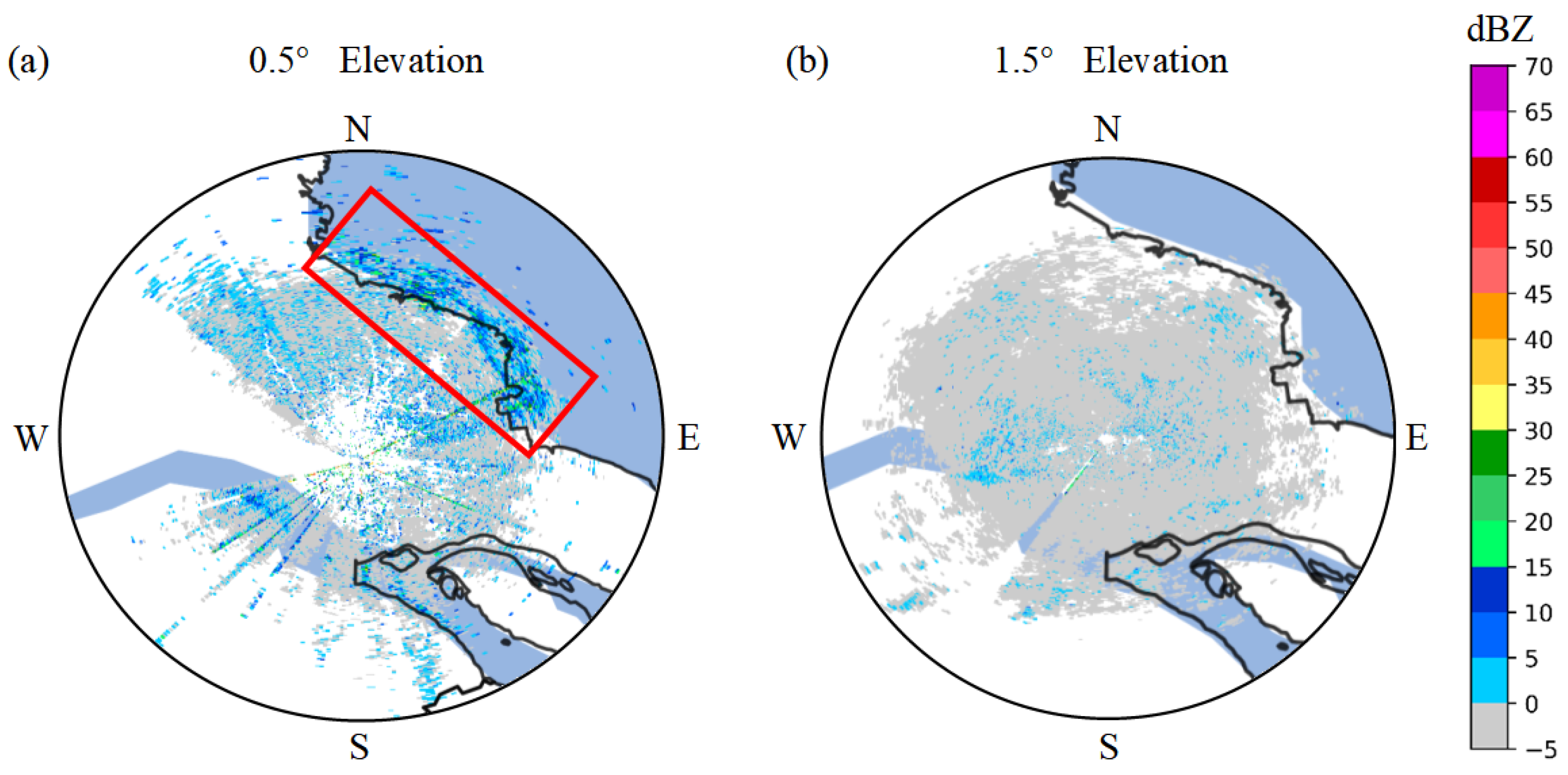
Figure 1. Wind turbine clutter captured by the CINRAD radar in Nantong City: (a) 0.5° elevation radar reflectivity echo; (b) 1.5° elevation radar reflectivity echo. (Red box represents the WTC area).
Electronics 14 03467 g001
Figure 2. Comparison of radar wind turbine clutter in 2008 and 2025 in Nantong City. (a) Radar reflectivity echo in 2008. (b) Radar reflectivity echo in 2025. (Red box represents the WTC area).
Electronics 14 03467 g002
Figure 3. Radar images captured at a 0.5° scan angle.
Electronics 14 03467 g003
Figure 4. The key procedures involved in generating a wind farm dataset, which encompass (1) dividing radar data into distinct blocks, (2) computing features related to wind turbine clutter for each block, and (3) assigning labels to samples according to the temporal and geographical coordinates of the wind farm, resulting in the formation of a wind farm dataset.
Electronics 14 03467 g004
Figure 5. The architecture of the Random Forest algorithm, which relies on the bagging (bootstrap + aggregating) technique.
Electronics 14 03467 g005
Figure 6. The overall workflow for training and optimizing the WTCDA-RF algorithm.
Electronics 14 03467 g006
Figure 7. The ranking of feature importance. Notably, the top 25 essential features score greater than 2.18.
Electronics 14 03467 g007
Figure 8. ROC curve.
Electronics 14 03467 g008
Figure 9. The distance between Nantong weather radar and the wind farm near Rudong County. The arrow indicates the radar’s location, while the wind farm is enclosed within a black polygon.
Electronics 14 03467 g009
Figure 10. WTC detection results under clear weather conditions (each black rectangle represents the center of a region identified by the algorithm, while the polygonal boundary encloses all detected points). (a) Reflectivity, (b) radial velocity, (c) spectrum width, (d) differential reflectivity, (e) correlation coefficient, (f) differential phase.
Electronics 14 03467 g010
Figure 11. WTC detection results under light rain conditions (each black rectangle represents the center of a region identified by the algorithm, while the polygonal boundary encloses all detected points). (a) Light rain, (b) Widespread light rain, (c) Moderate rain, (d) Widespread moderate rain, (e) Severe convective weather, (f) Severe convection turns into light rain.
Electronics 14 03467 g011
Figure 12. The WTC detection results for the Shangchuan Island Wind Farm (each black rectangle represents the center of a region identified by the algorithm, while the polygonal boundary encloses all detected points). (a) Reflectivity, (b) radial velocity, (c) spectrum width.
Electronics 14 03467 g012
Figure 13. The WTC detection results for the Changsha Wind Farm (each black rectangle represents the center of a region identified by the algorithm, while the polygonal boundary encloses all detected points). (a) Reflectivity, (b) radial velocity, (c) spectrum width.
Electronics 14 03467 g013
Figure 14. The WTC detection results for the Yantai Wind Farm (each black rectangle represents the center of a region identified by the algorithm, while the polygonal boundary encloses all detected points). (a) Reflectivity, (b) radial velocity, (c) spectrum width, (d) differential reflectivity, (e) correlation coefficient, (f) differential phase.
Electronics 14 03467 g014
Table 1. Newly incorporated body scanning modes for enhanced radar configuration.
Serial NumberObservation ModelNumber of Elevation AnglesVolume Scan CycleResolution RangeAdaptation Conditions
1VCP215D126 min460 km 125 mgeneral precipitation (fine resolution)
2VCP225D146 min460 km 125 mgeneral precipitation (fine resolution)
3VCP216D156 min460 km 62.5 mgeneral precipitation (ultra-fine resolution)
4VCP226D63 min330 km 62.5 mgeneral precipitation (rapid ultra-fine resolution)
Table 2. Confusion matrix for two-class classification.
Number of Elevation AnglesVolume Scan Cycle
Model predict classY (Yes WTC)TP (True Positives)FP (False Positives)
N (No WTC)FN (False Negatives)TN (True Negatives)
Column CountsPc = TP + FNNC = FP + TN
Table 3. Performance scores of the WTCDA-RF model on the test set.
ACCPREF1-ScoreG-MeanPODFARCSI
0.90920.89370.9110.9090.92890.10630.8365
Table 4. Evaluation metrics of WTCDA-RF under different weather conditions.
Weather ConditionPODFARCSI
Light rain0.8930.1150.824
Widespread light rain0.8720.1280.803
Moderate rain0.8320.1520.782
Widespread moderate rain0.8170.1680.767
Severe convective0.7930.1790.744
light rain0.8390.1470.789
Table 5. Model performance scores.
PODFARCSI
WTCDA-FL0.6870.2910.594
WTCDA-CNN0.7520.2260.683
WTCDA-RF0.7900.1820.748
Disclaimer/Publisher’s Note: The statements, opinions and data contained in all publications are solely those of the individual author(s) and contributor(s) and not of MDPI and/or the editor(s). MDPI and/or the editor(s) disclaim responsibility for any injury to people or property resulting from any ideas, methods, instructions or products referred to in the content.