Effect of Deep Recurrent Architectures on Code Vulnerability Detection: Performance Evaluation for SQL Injection in Python

Abstract

Security defects in software code can lead to situations that compromise web-based systems, data security, service availability, and the reliability of functionality. Therefore, it is crucial to detect code vulnerabilities as early as possible. During the research, the architectures of the deep learning models, peephole LSTM, GRU-Z, and GRU-LN, their element regularizations, and their hyperparameter settings were analysed to achieve the highest performance in detecting SQL injection vulnerabilities in Python code. The results of the research showed that after investigating the effect of hyperparameters on Word2Vector embeddings and applying the most efficient one, the peephole LSTM, delivered the highest performance (F1 = 0.90)—surpassing GRU-Z (0.88) and GRU-LN (0.878)—thereby confirming that the access of the peephole connections to the cell state produces the highest performance score in the architecture of the peephole LSTM model. Comparison of the results with other research indicates that the use of the selected deep learning models and the suggested research methodology allows for improving the performance in detecting SQL injection vulnerabilities in Python-based web applications, with an F1 score reaching 0.90, which is approximately 10% higher than achieved by other researchers.

1. Introduction

With the increasing complexity of modern software and the variety of potential vulnerabilities in source code, it has become nearly infeasible to detect them with static rules in code analysers. Software vulnerabilities are code-based defects that can be exploited by malicious actors, leading to unauthorised access to sensitive data and its misuse [1]. The consequences of such attacks can include loss of information or unauthorised disclosure of confidential information, manipulation, and systemic failure. Therefore, it is highly crucial to detect vulnerabilities in the code as early as possible. Although techniques exist to detect vulnerable code, improving their accuracy and effectiveness to a practically applicable level remains a challenge. Identifying potentially vulnerable code is crucial to improving the security of software systems. Today, traditional vulnerability detection methods for software code are used, such as static and dynamic analysis tools; however, their main drawback is the large number of false-positive and false-negative predictions [2,3]. However, these tools are based on rules and, therefore, are limited to engineers’ experience-based rules [4]. Traditional approaches based on manually defined rules are gradually being replaced by automated approaches empowered by data-driven methods [5]. The availability of large amounts of open-source code presents an opportunity to learn directly from mined data the patterns of software vulnerabilities [6]. Classical machine learning (ML) models are still recommended for most modelling tasks. However, the correct and accurate result depends on the data engineering and training processes and the structure of the ML model. This can lead to the removal of important information from the data set and impact the results of the ML model for vulnerability detection in source code [7]. Deep learning models (DL) can automatically extract the salient information from raw data and achieve optimal predictive performance. One type of code vulnerability is SQL injection, which has consistently ranked among the top three threats in the Top 10 reports of the Open Web Application Security Project (OWASP) from 2013 to 2021. This suggests that vulnerability detection remains ineffective.

When large language models began to be used for code generation in web-based system development, research by authors of [8] revealed that SQL injection vulnerabilities persisted in the code they generated. Based on these facts, our research aims to investigate the performance of deep learning (DL) models in detecting SQL injection vulnerabilities in Python code. The suggested DL model allows us to improve the detection of vulnerable code much more effectively. The main contributions of our research are as follows:

• Improved performance for detecting SQL injection vulnerabilities in Python-based web applications using a deep recurrent architecture, considering their architectural features.
• A systematic analysis of Word2Vector embedding hyperparameters revealed the optimal configuration that maximises vulnerability detection performance.
• Evaluated peephole LSTM and modified GRU architectures (with layer normalisation and zoneout) for SQL vulnerability detection in the system development code base.

The remainder of this research paper is structured as follows. Section 2 provides an overview of the related work. Section 3 presents a research methodology, Word2Vector model investigation, and RNN architectures research. Section 4 presents the results and a discussion. Section 5 describes threats to validity. Finally, Section 6 concludes the paper.

2. Related Works

Data comprise one of the most important assets that must be preserved and protected; therefore, databases in web-based systems should protect this data from unauthorised access. Based on the foundation OWASP Top 10 [9] and Common Weakness Enumeration lists [10], SQL injections are among the top security vulnerabilities that threaten data security in web applications. Web-based system functionalities, such as login pages, product request forms, feedback forms, search pages, and dynamic content delivery, shape modern websites’ need to communicate with users [11]. The security issue is that web-based system fields for user input allow SQL statements to pass through and query the database directly. This allows access to data or files that should not be accessible, or adding statements, changing or destroying databases [12]. SQL injection is a type of vulnerability in the source code. SQL injection attacks are one of the oldest, most prevalent, and most damaging security attacks facing web-based systems. Detecting this vulnerability has been proposed using various methods: static, dynamic, or hybrid analysis, as well as ML and data mining techniques [2]. The main issue arises when code-based software metrics (such as cyclomatic complexity, lines of code, developer activity, and churn metrics) are used to predict software vulnerabilities [13]. Several research studies show that software metrics are inadequate due to their high rate of false positives [2,3].

Due to the wide availability of open-source software code repositories, it has become possible to use these data in data-driven methods, allowing the automation of vulnerability detection in software code [14,15].

Researchers perform SQL injection detections in two ways. First, SQLi, where the data set consists only of SQL queries [16,17] and achieves a performance score of approximately 0.99. The second—SQL queries as code snippets are found in the whole system’s development code base. The second way requires more effort to detect SQL injections because to extract and catch SQL injections in the code base, one must mine relatively scarce and noisy labels from vulnerability fixing commits, leading to pronounced class imbalance and label uncertainty. Similar research on SQL injection detection in code base was carried out to detect software code-based vulnerabilities with synthetic and/or real data sets in different programming languages (C/C++, Java and PHP) for web-based system development. The researchers proposed a model with synthetic datasets, achieving an accuracy of 57% to 90% [18,19,20,21]. However, when developers leave vulnerabilities, synthetic data sets do not reflect real code [22]. Thus, we decided to analyse only research conducted with real code datasets.

Table 1. The summary of the different deep learning models used in detecting vulnerabilities in the Python codebase.

Authors	Research Objective	Vector Embedding Model	ML Model Used	Performance (F1 Score)
Bagheri & Hegeds (2021) [23]	Evaluate different source code representation methods for vulnerability prediction.	Word2Vector, FastText, BERT	LSTM	0.84–0.86 of all code vulnerabilities
Wartschinski et al. (2022) [24]	Propose the DL model for a vulnerability detection system that automatically learns features of vulnerable code from a large, real-world codebase.	Word2Vector	LSTM	0.80–0.90 of all code vulnerabilities; 80.1% of SQL injection vulnerabilities
Wang et al. (2024) [25]	Evaluate the effects of DL architectures derived from combinations of representation learning models on code vulnerability detection.	Word2Vector, FastText, Code-BERT	LSTM, XGBoost, GRU, CNN, MLP	0.78- 0.88 of all code vulnerabilities.
Tran et al. (2025) [26]	A statement-level code vulnerability detection.	BERT	GNN-based models	0.74 of all code vulnerabilities.

compares several studies that used different deep learning models to detect vulnerabilities in Python code. This study was compared only with real data sets from the GitHub platform for code vulnerability detection.

The analysis performed on related work showed (see Table 1) the variety of embedding models used for ML models: Word2Vector [27], Code-BERT [28], BERT [29], and FastText [30]. Researchers of [23,24,25] selected Word2Vector as the main or one of the main embedding models in the data preparation set for input to ML algorithms, while other studies used additional embedding models such as Code-BERT, BERT, and FastText. When analysing these publications and their experiments more closely, we identified two aspects related to preferences for vector embedding models. The first aspect is that the prediction model based on the Word2Vector representation of the code outperformed models based on FastText and BERT to detect SQL injection [23] and it was more stable than other models [25]. The second aspect is that BERT or Code-Bert models have large-scale, complex architectures and require large amounts of data and powerful resources. Previous work considers embedding model choice, but they do not investigate which hyperparameters matter and how they influence the performance score.

Deep learning models, such as LSTM and GNN-based architectures, are the most commonly used in code vulnerability detection research. The analysed works use standard LSTM/GRU or GNNs, but they do not analyse how their recurrent architectural elements and their regularisations affect code vulnerability detection’s performance. Analysis of related works (see Table 1) reveals that they achieve performance scores (F1) ranging from 0.74 to 0.90 for various code vulnerability detection tasks, producing competitive and promising results.

3. Design and Evaluation of RNN Architectures for SQL-Injection Detection

Section 3 investigates the main research question of how recurrent neural network architectural choices affect SQL-injection detection performance (F1) on real and unbalanced Python code data sets. We carried out two investigations.

3.1. Research Methodology

The first investigation consists of experimenting with different sets of hyperparameters of the Word2Vector model, which we determined for this model training. Researchers of [23] analyse the influence of hyperparameters on performance score, but they do not investigate these hyperparameters with different numbers of epochs. The second investigation involves experimenting with the architectures of the DL model using various values of the hyperparameters of the DL model. In our research, we decided to use less studied variations in LSTM and GRU deep learning models, such as peephole LSTM, GRU-R, and GRU-LN, and evaluate their performance in detecting code vulnerability.

For our investigation, we used the SQL injection vulnerability data set from the VUDENC collection [31]. The main principle of code sample generation is the analysis of the revisions of source code projects in GitHub code repositories. According to scientific work of [32], code vulnerabilities can be detected by analysing GitHub revisions and their associated commit messages. Authors of [31] went through commits with keywords in the commit messages that were indicative of a vulnerability fix. The parent version of each file that existed before the vulnerability-fixing commit was flagged as vulnerable because it contained the vulnerability that needed to be fixed. Using diff files, which list the source code-level changes made between two successive commits, allowed us to extract the exact lines that were repaired and, therefore, determine which lines were vulnerable. Based on this methodology, the data set was created with vulnerable and non-vulnerable code snipped from the Python code, and based on this information, they were labelled. In the chosen data set, 17.86% were labelled as vulnerable code samples of all the gathered code samples. With this distribution of code sample labels, the applied data set is large enough, but is imbalanced between classes, clean code, and vulnerable SQL injection code. The problem of learning from imbalanced datasets is related to an imbalance in the distribution of training data, which often causes learning algorithms to perform poorly in the minority class [33]. The common solution is to sample the data before training to rebalance the class distribution. Since the data set is imbalanced, classes should be weighed accordingly [33,34]. The balancing function (class_weight) was applied during deep learning model training, where weights are automatically adjusted inversely proportional to the frequency of classes in the input data. The weights were inversely proportional to the frequency of each class, ensuring that the model does not ignore the vulnerable code samples. This helps avoid biasing the model towards a dominant class and improves overall performance.

In our data set, most of the labels are marked as non-vulnerable, and the ratio between the two classes is imbalanced. According to [35], in unbalanced data, the commonly used accuracy metric yields misleadingly high values that result from systematically predicting the class. In this way, in our research, the effect of the effectiveness of deep learning models was measured only by the performance score F1.

The proposed research consists of four steps: (1) preparation of a Python codebase for Word2Vector embedding; (2) investigation of Word2Vector model hyperparameters; (3) investigation of deep learning models using hyperparameters; (4) evaluation results of deep learning models (see Figure 1). The first and second steps are described in the following subsections, while the third and fourth steps are covered in the next subsections.

3.2. The Preparation of the Data Set for Word2Vector Embedding

The initial step (see Figure 1) involves converting raw text into vector representations using word embeddings [27,36]. Word2Vector, a neural network-based word embedding method, can capture semantic similarity between words using generated vector representations. The Word2Vector algorithm focuses primarily on representing each word as a vector and captures the semantic similarity of words through the cosine similarity of these vectors [37]. Researchers of [38] experimented to comparatively evaluate the capabilities of natural language feature extraction models (BERT-LSTM, Word2Vector-LSTM, GRU, CNN) in detecting SQL injection vulnerabilities. The Word2Vector-LSTM model had the shortest training time (198.62 s), while the training times for BERT-LSTM, GRU and CNN were more than 204 s. [38]. These aspects and the minimisation of computation resources motivated us to choose the Word2Vector embedding technique to encode Python code into tokens. First, in pre-processed Python code, we use word tokenisation, transforming each code snippet into a list of tokens (“for” and “init”, etc.). The tokens are then entered into a Word2Vector representation learning model to generate a word embedding matrix, ensuring that each token has a unique vector. The Word2Vector model was tested using a similar token comparison function from the Gensim library, which uses the cosine similarity metric to determine the similarity between two tokens. In summary, the Word2Vector model maintained similarities between Python code tokens, ensuring that semantic relations are preserved and making SQL injection code 200-dimensional vector representations suitable for our research to ensure the model’s ability to distinguish subtle meanings [39]. The data set has been partitioned into training categories. (80%) and testing (20%) sets. After the DL models learn to detect vulnerable code, the test data evaluates the model’s performance.

3.3. Investigation of the Hyperparameters of the Word2Vector Model

Before DL models could detect SQL injection vulnerability in Python code, hyperparameter optimisation was performed to achieve the best performance of Word2Vector. In this way, the second step is to investigate the Word2Vector model, where experiments were conducted with different hyperparameters of the model. This experiment used a university computer, the characteristics of which AMD Ryzen 5 5600X, 6 Cores, 16 GB RAM, and NVIDIA GeForce RTX 3060Ti, 8 GB graphics card.

In this experimental investigation, the hyperparameters were chosen as follows:

• Number of iterations. The number of iterations refers to the number of batches required to complete the epoch.
• Vector size. When Word2Vector is used, the tokens are transformed into numerical vectors of specified sizes. Increasing the size of these vectors adds more axes to the positioning of words relative to each other, allowing the Word2Vector model to capture more complex relationships.
• Minimum count. The minimum count determines how often a token must appear in the training corpus to be assigned a vector representation. Tokens that appear less frequently are ignored and not encoded. Later, these types of tokens are ignored when complete lists of tokens are converted into lists of vectors.

The investigation of the hyperparameters of the Word2Vector model was carried out using the DL model LSTM with the following hyperparameters (base model): dropout size −0.2, the number of neurons is 100, the optimisation algorithm “adam” and batch size is equal to 128. It is important to mention that the selected parameters of the base ML model are not optimal, but they are suitable for determining how changing the hyperparameters affects the performance of the Word2Vector model. The F1 measure is used to evaluate performance because it is less influenced by a large number of true negatives and is better suited for class-imbalanced data sets.

The investigation of the hyperparameters of the Word2Vector model consisted of the following steps:

• Of the three hyperparameters, vector size, number of iterations, and minimum count, 80 combinations were created. These included:
  • the number of iterations $t\in \left\{40, 80, 120, 160\right\},$
  • vector sizes $v\in \left\{10, 100, 150, 200\right\},$
  • minimum counts $m\in \left\{1, \mathrm{10,100}, 1000, 4000\right\}.$

To create all possible combinations, Shapley values are employed as a measure of importance, indicating the significance of each parameter’s contribution [40]. The ranking is based on the Shapley value [41], a well-known concept from game theory, to estimate the importance of each feature for the task at hand, specifically taking into account interactions between features. The influence of the hyperparameter is defined by the Shapley value in Equation:

$${\varphi }_i(f, x)={\sum }_{S\text{⊆}\mathrm{F}\backslash \left\{\mathrm{i}\right\}}{\displaystyle \frac{\left|S\right|!\left(\left|F\right|-\left|S\right|-1\right)!}{\left|F\right|!}}\left[f_{S\cup \left\{i\right\}}\left(x\right)-f_S(x)\right]$$

(1)

where φ_i (f, x) is the Shapley value of the hyperparameter, which is determined as the average of its contributions across all possible permutations of the complete set (F) of {v,t,m}. Index i is the index of the hyperparameter whose contribution we want to measure, x is a particular hyperparameter tuple, and S is a subset that does not contain one of the three hyperparameters.

The objective is to analyse the impact of each hyperparameter, signifying its contribution towards attaining the best performance score F1 for the Word2Vector model. For each Word2Vector hyperparameter combination, we trained a base model LSTM model to detect vulnerabilities and recorded the F1 score. These 80 F1 scores form the basis for the Shapley value computation. The Shapley values are presented in

Table 2. Shapley values of the minimum count of the hyperparameter.

Minimum Count’s Values	Min	Max	Mean
1	0.004052	0.004052	0.004052
10	0.003995	0.003995	0.003995
100	0.003424	0.003424	0.003424
1000	−0.00229	−0.00229	−0.00229
4000	−0.02134	−0.02134	−0.02134

,

Table 3. Shapley values of the number of iterations of the hyperparameter.

Number of Iterations’ Values	Min	Max	Mean
40	0.005475	0.005475	0.005475
80	0.001825	0.005475	0.001825
120	−0.00183	−0.00183	−0.00183
160	−0.00548	0.005475	−0.00495

and

Table 4. Shapley values of the hyperparameter’s vector size.

Vector Size’s Values	Min	Max	Mean
10	−0.09699	0.09699	−0.09699
100	−0.03781	−0.03781	−0.03781
150	−0.00548	−0.00493	−0.00493
200	0.005475	0.027946	0.023789

.

2.

Based on Shapley values, an analysis was conducted that the greatest impact on the performance of the Word2Vector model was derived when the vector size value was highest (see Table 4, last row). In contrast, the lowest impact was observed when the minimum count value was the lowest (see Table 2, the first three rows), and the highest Shapley value was when the number of iterations ranged from 40 to 80 (see Table 3, the first two rows). Accordingly, it was decided to run only 32 combinations with a continuously augmented count of epochs: 40, 80, 120, 160.

3.

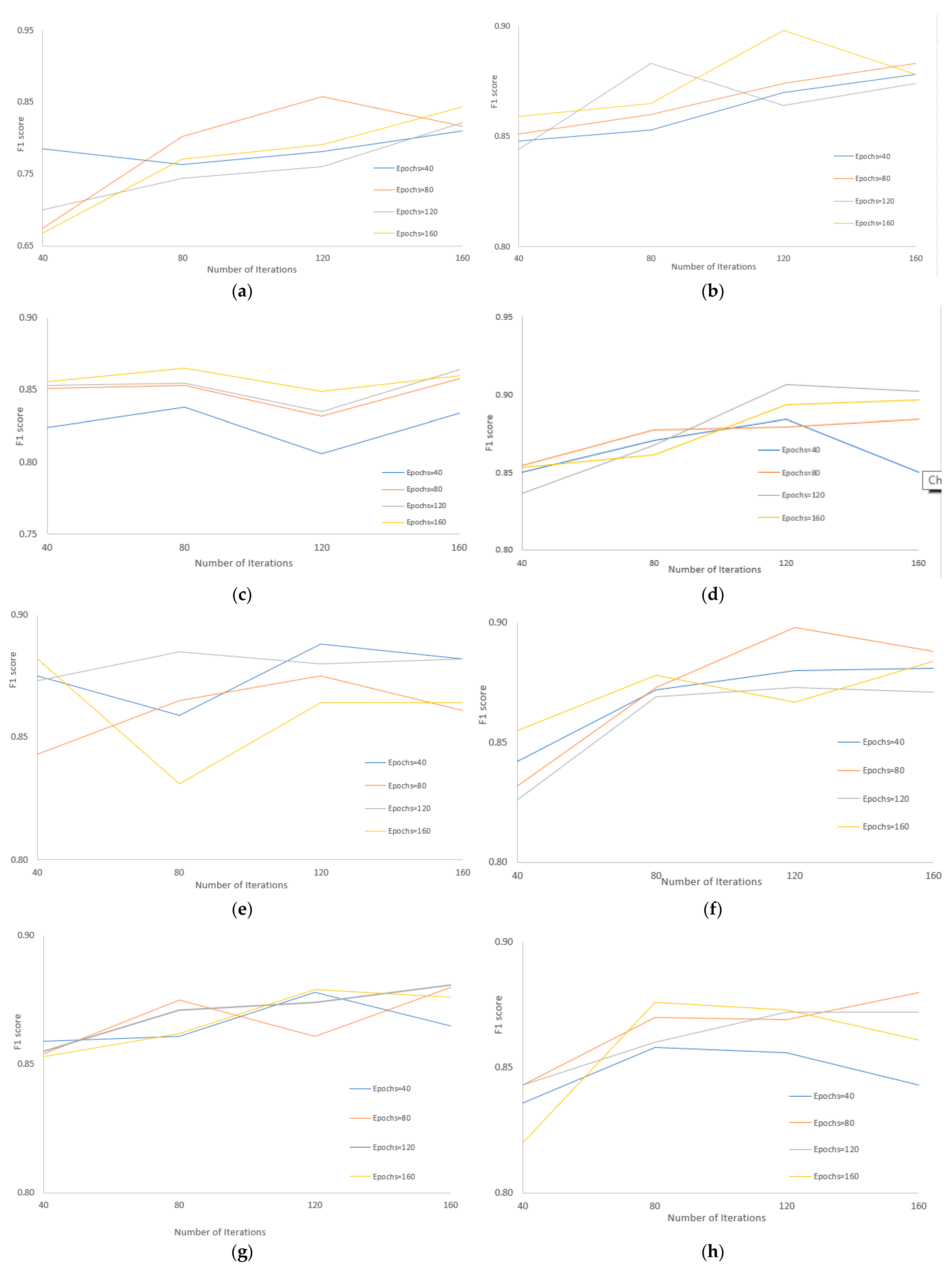
Word2Vector model performance (F1 score) was evaluated for each 32 combinations of hyperparameters (vector size, minimum count, number of iterations) with different numbers of epochs. The results of this investigation are presented in Figure 2.

Figure 2 presents the F1 score values for each of the 32 combinations, consisting of minimum count, vector size, and number of iterations. Summarising the results, it can be concluded that most of the hyperparameter combinations of the Word2Vec model performed well enough, with F1 scores greater than 0.8, except when the minimum count was 1 and the vector size was 10 (see Figure 2a). The lowest F1 score, 0.675, was achieved with the following combination of hyperparameters: minimum count = 1, number of epochs = 40, and vector size = 10 (Figure 2a). On the other hand, the highest F1 score of 0.906 was achieved with the following combination of hyperparameters: minimum count = 1, number of epochs = 120, vector size = 200 (Figure 2d). From the investigation, it was observed that the main hyperparameter that led to such different results was the vector size. Therefore, it can be concluded that this hyperparameter strongly influences the performance of the Word2Vector model. Another hyperparameter of the Word2Vector model whose influence on the performance of the Word2Vector model has a minimum impact is the minimum count. We tested five different values of this hyperparameter: 1, 10, 100, 1000, and 4000, and observed that the most efficient case was with a minimum count of 1, achieving the best F1 score of 0.906 (Figure 2d). Another best score, 0.872, was achieved with hyperparameters identical to the best-performing test case, but with a minimum count of 4000 (Figure 2g). When comparing the F1 scores of these two cases, which differ by 0.034, it can be concluded that the most effective minimum count in the study is equal to 1. Before research, it seemed reasonable to assume that ignoring rare tokens would improve performance. However, the results showed that this assumption was incorrect, as the model performs better when hardly any tokens are ignored.

The last hyperparameter studied was the number of training epochs for the Word2Vector model. The increase in the number of epochs from 40 to 80 was found to improve the F1 score. However, when the number of epochs of 120 and 160 was tested, the results became less stable. For example, in the test cases (see Figure 2e), the Word2Vector model with 120 epochs performed better than the model with 160 epochs. A similar trend was also observed in test cases where minimum count = 1000, vector size = 200 (Figure 2g). The performance difference between the number of epochs 120 and 160 usually varies between 0.001 and 0.03. Therefore, with limited computational resources, enough good results can be achieved in 120 epochs.

Investigation of the Word2Vector model with the base DL model shows that the best F1 performance score of 0.906 was achieved with minimum count = 1, vector size = 200 and number of iterations = 120 (Figure 2d).

3.4. Recurrent Neural Network Architectures Analysis for SQL Injection Detection

For our research, we decided to apply variations in the DL models of LSTM and GRU. Their selection was based on the analysis of related work (see Table 1), which showed that LSTM and GRU achieved significant results. In this research, we decided to try variations in LSTM and GRU to improve the performance of SQL injection vulnerability detection. They are more complex in structure, and we hypothesise that they could achieve improved performance for this type of task.

The input of LSTM consists of two parts: the input xt of the current time t and the output at the previous time t − 1. If the output is turned off at time t, the output of the network at time t will be 0 [42]. So, the input of the gate will be completely related to the input xt, but the historical information will be lost. One of the decisions is to add peephole connections to all gates in the same LSTM, so that all gates can detect the current cell state even when the output gate is closed [43]. Peephole LSTM was chosen because researchers of [43,44] found that peephole connections allow LSTM cells to better capture long-term dependencies in sequences.

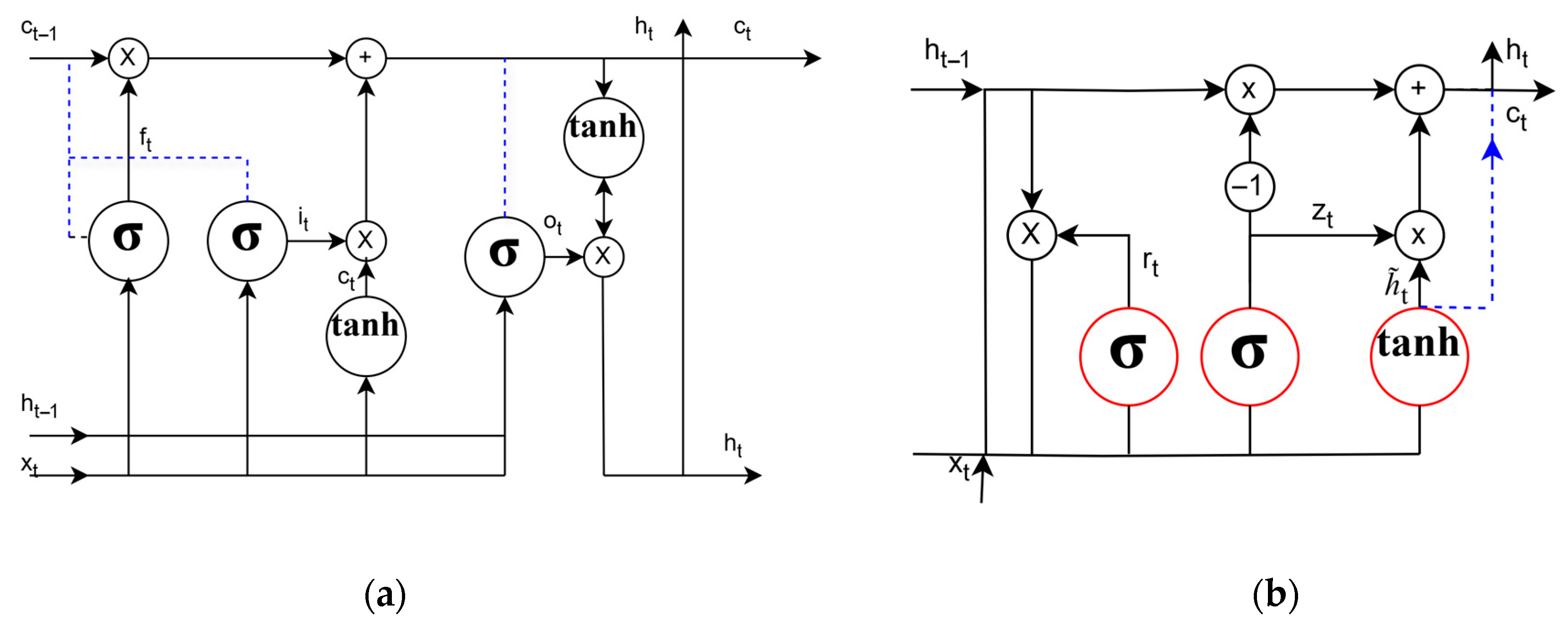
An LSTM peephole architecture is implemented by making peephole connections (see Figure 3a). Gates can be used not only on the input layer xt and the hidden previous state ℎ_t−1, but also on the preceding internal state c_t−1, which adds another term to the gate equations that also comes back from the cell ct, and the forget gate f_t is generated by the activation function [42]. All gates, and (f_t, i_t, o_t) can detect the current cell state even when the output gate is closed. The forgetting gate’s output, which allows for forgetting to hide the state of the cell in the top layer, is evaluated using the sigmoid output, which has values between 0 an output of the forgetting gate’s output, which the allows for forgetting to hide the state of the cell in the top layer, is evaluated using the sigmoid output, which has values between 0 and 1. The mathematical expressions of gates f_t, i_t, and o_t are presented in Equations (2)–(4).

$$f_t=\sigma (W_f{x}_t+W_f{xh}_{t-1}+W_f{c}_{t-1}+b_f$$

(2)

$$i_t=\sigma (W_i{x}_t+W_i{xh}_{t-1}+W_i{c}_{t-1}+b_i$$

(3)

$$o_t=\sigma (W_o{x}_t+W_o{xh}_{t-1}+W_o{c}_{t-1}+b_o$$

(4)

where W_f, W_i, W_o, are weight matrices, and b_f, b_i, b_o are bias vectors.

Classification of SQL injection vulnerabilities in Python code requires modelling long-sequence dependencies: Python programming language implementations, input parameters may be assigned, threaded through several functions, so the model must remember the long flow: at each time step, letting the network recall when and where user input first entered the data flow, track it through reassignments and joins. One of the disadvantages of this model is the severe risk of overfitting due to additional complexity when the model is trained with a small or noisy dataset, so the hyperparameters of the ML model, such as dropout, must be specially adapted to the data.

Two variations were chosen from the GRU DL models: a GRU model with layer normalisation (GRU-LN) and a GRU model with a zone-out hyperparameter (GRU-Z). The GRU-LN architecture injects layer normalisation directly into the affine transformations of the update z_t, reset r_t, and candidate ℎ̃_t gates, stabilising activations at every time step rather than across the mini-batch connections (see Figure 3b). The mathematical expression of gates z_t, r_t, ℎ̃_t is presented in Equations (5) and (6).

$$z_t=r_t=\sigma \left(LN\left(W_h{h}_{t-1}\right)\right)+\sigma \left(LN\left(W_x{x}_t\right)\right)$$

(5)

$${\mathrm{h}̃}_t=tanh(LN\left(W{x}_t\right)+r_t⨀LN(W_{h-1}\left)\right)$$

(6)

The normalisation in the layers ensures consistent input to each layer and makes the learning process more stable: it lets remember vulnerable variables or values across several code lines and still trains stably on the small datasets common in SQL injections in the Python codebase. Improved learning stability was the main advantage compared to the standard GRU model.

Zoneout is a special case of dropout, where ℎ̃_t is the hidden activation without zoneout, and the hidden state h_t has zoneout applied stochastically as represented by the dashed blue line connections (see Figure 3b). This can be seen as a dropout on the corresponding input node, which represents the difference ℎ̃_t−h_t-1. The zoneout hyperparameter to stochastically determine whether the hidden state h_t and the cell state c_t at a time step should be updated or retained from the previous time step h_t−1, which allows the model to selectively store relevant information from previous parts of the SQL query, enabling it to capture complex attack patterns over long sequences without overloading the model with unnecessary information [45]. Unlike dropout, zoneout acts as a temporal skip connection, letting information flow unchanged across time. Another aspect of the GRU-Z selection was the ability of the zoned output to maintain temporal consistency [46], which is important for tasks such as detecting vulnerabilities in program code, as it relies on the continuity and preservation of consistent data in memory.

These recurrent neural network architectural modifications, peephole LSTM and GRU-LN, GRU-Z, were designed to address limitations in standard RNNs and improve performance in tasks requiring them to better model dependencies, which is especially crucial for challenging tasks like program code analysis or anomaly detection. DL model’s architectures, peephole LSTM and GRU-LN/GRU-Z, allowed us to enable them to better model long-term dependencies in sequences (dropout/zoneout and learning rate hyperparameters.

3.5. Deep Learning Models Investigation

Our experiment to find the best hyperparameter combination for each DL model started with the initial set of hyperparameters of the base model (see

Table 5. Hyperparameters and their values in the experiment.

Name of Hyperparameter	Description and Values in the Experiment
Number of neurons	Neurons perform complex computations during training that allow ML models to recognise complex relationships between data and make predictions based on input. A higher number of neurons increases the training time. Initial value = 10. During the experiment, values from the interval [1, 200] were used.
Dropout	A regularisation hyperparameter of an ML model, where random neurons are ignored during training to avoid overfitting. This improves the performance of the model by reducing interdependencies between neurons and increasing robustness when handling new unseen data. Initial value = 0.2. During the experiment, the interval values [0, 0.6] were used.
Optimizer	Optimizer is one of the most important hyperparameters of an ML model, as it determines how the model learns and updates its parameters during learning to minimise the loss function. Initial value = “adam”. During the experiment, the values from the list [“adagrad”, “adam”, “nadam”, “rmsprop”, “adamax”, “adadelta”, “ftrl”] were used.
Number of epochs	The number of epochs determines how many times the entire data set is passed through during training. Choosing the correct number of epochs is critical because it affects how well the model learns the relationships in the data set. Initial value = 15. During the experiment, values of the interval [40, 320] were used.
Batch Size	Batch size defines the number of samples processed by the ML model during training before updating its parameters. This hyperparameter is important because it affects the learning speed and memory usage, which are important to balance model performance and computational speed. Initial value = 250. During the experiment, the values from the interval [8, 1024] were used.
Zoneout	Zoneout is a state-of-the-art method for regularising RNN by stochastically preserving previous hidden activations [46]. Zone-out can improve performance by capturing longer-term dependencies compared to GRU. Initial value = 0.2. During the experiment, the values of the interval [0, 0.6] were used.

). It is essential to note that the selected hyperparameters of the base model are not optimal; however, they are suitable for determining how changes in the hyperparameters affect the DL model’s performance.

The steps of this investigation are presented in Figure 4 and were performed with the following DL models: peephole LSTM (30 times), GRU-LN (30 times), and GRU-Z (38 times). The differences in the number of times are because peephole LSTM and GRU-LN involved tuning six hyperparameters (number of neurons, dropout, optimiser, number of epochs, batch size, zone-out), while GRU-Z included an additional zone-out hyperparameter.

During the experiment, the value of only one hyperparameter was changed at a time, while all other hyperparameters remained static (see Figure 4). This way was decided because by altering only one hyperparameter at a time, it becomes easier to directly attribute performance changes to that specific hyperparameter (the impact of each hyperparameter on the F1 score can be seen in Figure 5). This way helps isolate the impact of each hyperparameter on the model’s performance, leading to a clearer understanding of its effect.

As determined in the analysis of related study [24], a larger number of epochs can lead to better results because the model absorbs information more efficiently. However, since it will be necessary to test many different combinations of hyperparameters with three different models, we will use these basic ones to evaluate the influence of the hyperparameters, and only the best-performing combination of hyperparameters with larger numbers of epochs will be studied. It is important to mention that the search for the most efficient combination will be carried out with 15 epochs, since the number of combinations that will be explored is large enough. This process of establishing hyperparameters for DL-based models will be repeated with the peephole LSTM, GRU-Z, and GRU-LN models.

After investigating various hyperparameter values and evaluating their impact on the base model, the two highest-performing values of each hyperparameter category of the ML model were selected. These selected hyperparameters will be included in the final investigation phase, which will search for the best-performing model capable of detecting SQL injection vulnerabilities in the Python code of the web-based system. Based on F1 scores, the two best-performing combinations for each DL model architecture will be tested with a different number of epochs.

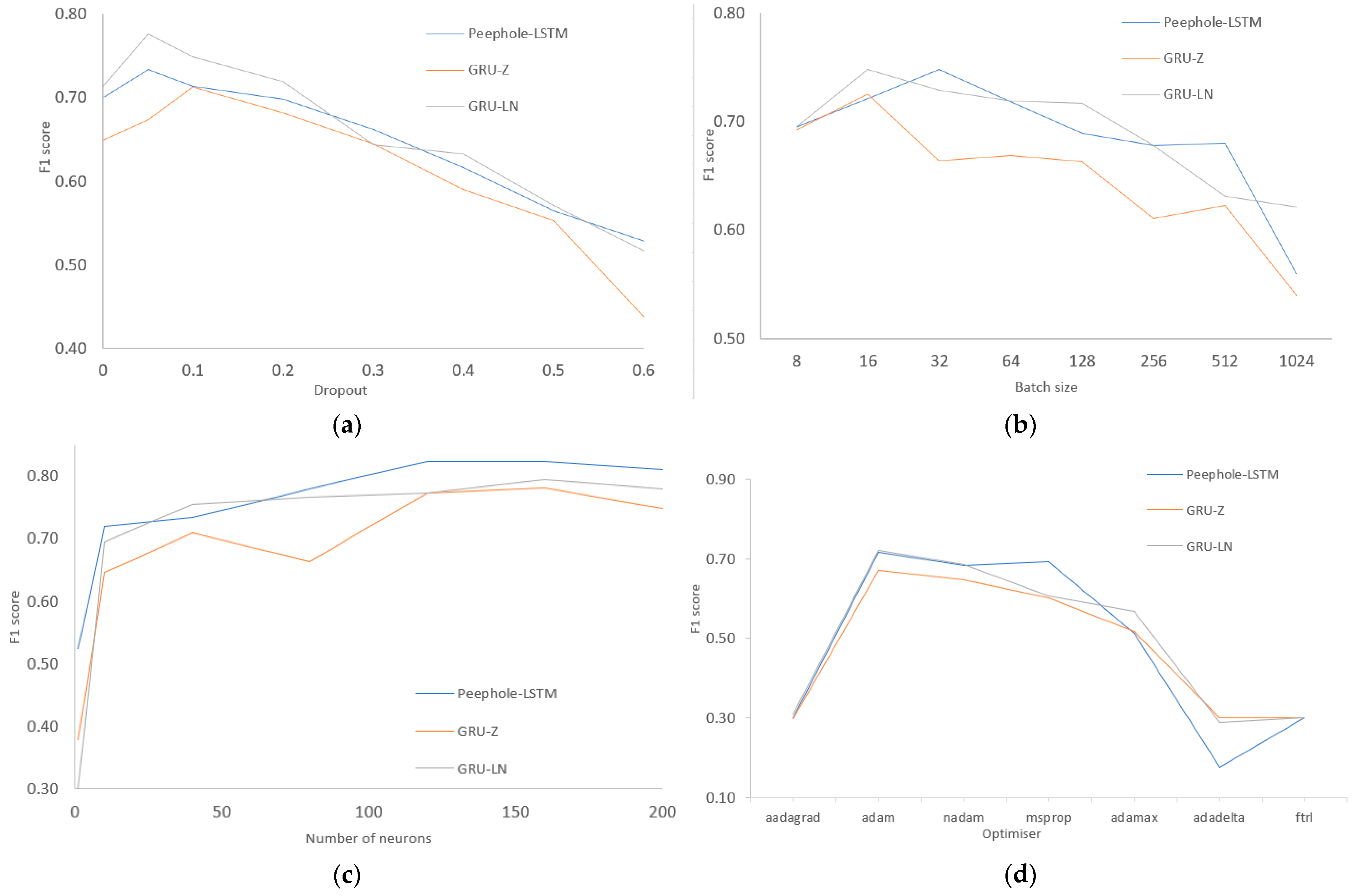
As seen in Figure 5, the base model with initial model hyperparameters showed the best performance with dropout values of 0.05 and 0.1, achieving F1 scores of 0.74 and 0.776 for the peephole LSTM and GRU-LN models (see Figure 5a). It was observed that with dropout values ranging from 0.3 to 0.6, the performance of the model steadily decreased, with a 0.206 difference between the best and worst models (see Figure 5a). This allows us to draw an initial conclusion that the dropout values strongly influence the overall performance of the model.

According to the number of neurons (Figure 5b), the performance of the model with 120 and 160 neurons ranged from 0.83 to 0.824. It is important to mention that the performance of the model deteriorated when we increased the number of neurons to 200. The batch sizes were 16 and 32, with the base model based on DL reaching a performance of 0.721 to 0.748, and the F1 score steadily decreased with a batch size of 1024, reaching 0.566 (Figure 5c).

Depending on the optimiser (Figure 5d), the base DL model achieved the best performance with the optimisation algorithms “adam” and “rmsprop”, achieving F1 scores of 0.692 and 0.715. The next closest algorithm was “nadam”, which achieved an F1 score of 0.683. The rest of the optimiser algorithms were inefficient, with the worst being “adadelta”, which achieved performance ranging from 17.6% to 30% in each DL model.

We concluded that zone output increases F1 in the GRU-Z model when the zoneout hyperparameter is 0.1 to 0.3. If the zoneout value is unused or exceeds 0.3, the model’s F1 score decreases. At a zoneout value of 0.4, the F1 score was 0.652; at 0.5, the F1 score reached 0.644; and the lowest F1 score, 0.611, occurred with a zoneout value of 0.6. We concluded that zone output increases F1 in the GRU-Z model. During the experiment with the DL models, two values of each model were found to influence performance. The second step is to choose two hyperparameter combinations that perform best for each model and test them with different numbers of epochs, ranging from 40 to 320.

To mitigate bias from class imbalance, we employed weights automatically adjusted inversely proportional to the frequency of classes in the input data, and all results were evaluated only by the performance score F1 as the main metric. Overfitting was addressed through regularisation of hyperparameters: we systematically varied dropout (0–0.6) for all architectures and zoneout (0–0.6) for GRU-Z, and selected configurations within the stable range of dropout (≈0.05–0.1), since higher rates (>0.3) degraded F1.

The observed performance differences are meaningful (see Figure 6) and were proven by paired F1 comparisons at the same number of epochs (40–320) in

Table 6. Paired F1 differences between DL models.

Number of Epochs	F1 of Peephole LSTM	F1 of GRU-LN	F1 of GRU-Z	ΔF1 (Peephole LSTM—GRU-LN)	ΔF1 (Peephole LSTM—GRU-Z)
40	0.864	0.837	0.851	0.027	0.013
80	0.873	0.844	0.856	0.029	0.017
120	0.878	0.853	0.865	0.025	0.013
160	0.889	0.874	0.88	0.015	0.009
200	0.894	0.878	0.876	0.016	0.018
240	0.9	0.869	0.872	0.031	0.028
280	0.897	0.867	0.867	0.03	0.03

.

Peephole LSTM consistently outperforms GRU-LN and GRU-Z when the same number of epochs. This indicates that the peephole LSTM is reliably better than both GRU-LN and GRU-Z. The mean F1 gains (~+0.02–0.03) are statistically significant. A paired t-test on these differences shows that peephole LSTM significantly outperforms GRU-LN (mean ΔF1 = 0.026695 and 95% CI [0.0198, 0.0334] and GRU-Z (mean ΔF1 = 0.0204, 95% CI [0.0125, 0.0282]). This proves that peephole LSTM is the more suitable RNN architecture for SQL-injection detection, when the number of epochs is between 200 and 240 and allows one to avoid the overfitting behaviour you observed for GRU-Z after ~160 epochs.

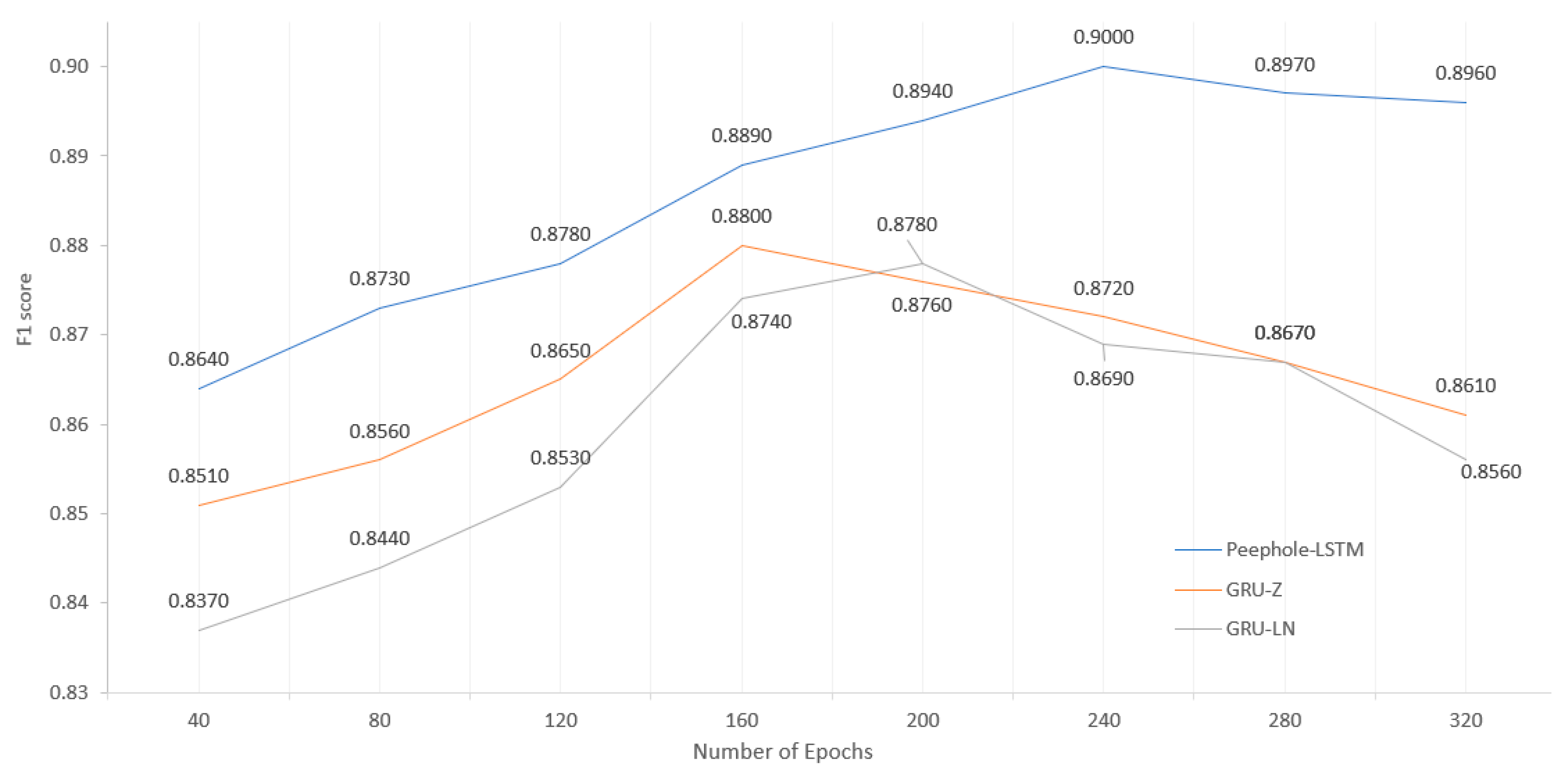
Figure 6 illustrates the clear impact of the number of epochs on the performance of the model. The results reveal that the peephole LSTM model achieved its highest F1 score of 0.90 at 240 epochs. The model’s performance steadily increased from 40 to 240 epochs, but a slight degradation in performance was observed between 280 and 320 epochs. The GRU-Z model performed reasonably well in all numbers of epochs, achieving an F1 score of 0.85 even at the lowest epoch count. The reason for the deterioration in model performance after 160 epochs is overfitting. The GRU-LN model achieved the highest result with 200 epochs, where the F1 score reached 0.878. The model’s performance steadily increased from 40 to 200 epochs but experienced deterioration between 240 and 320 epochs.

4. Results and Discussions

In the chosen SQL injection vulnerability data set, we investigated three DL models to determine the best performance in detecting vulnerable Python code. Before that, we trained the Word2Vector model and searched for the combination of hyperparameters that allowed us to achieve the best performance score. Our research reveals the outstanding results of the peephole LSTM model, which outperformed both the GRU-LN and GRU-Z models in all epoch counts. The peephole LSTM model with added peephole connections (exposing the cell state to all gates) performed the best, with an F1 score reaching 0.90. The next model that performed the best was GRU-Z, with an F1 score of 0.88. The result obtained was influenced by the GRU-Z architecture, characterised by an injecting zone-out that acted as a temporal skip connection that stochastically preserves prior hidden states. Applying layer normalisation to GRU-LN gates stabilised training on limited data and yielded smooth learning curves with fewer signs of overfitting. The model reached F1 = 0.87 at ≈200 epochs, converging slightly later than GRU-Z but earlier than peephole LSTM. Its peak F1 was narrowly below GRU-Z, suggesting that while normalisation improves optimisation stability, it did not confer the same degree of generalisation benefit as zoneout for this task. As with the other models, the smaller batch size (16) and the low dropout were consistently favourable.

The difference in results between peephole LSTM and GRU-Z is 0.02, and between peephole LSTM and GRU-LN is 0.022. The results are logical, as the study used a more complex variation in the LSTM architecture (peephole LSTM), which includes additional connections between nodes to facilitate more efficient information absorption. After investigating the results of the GRU variation models (see Figure 6), it can be observed that their performance is similar, with the GRU-Z model being 0.2% more efficient than the GRU-LN. Furthermore, it can be seen that the GRU models’ results have a greater difference in smaller epochs (40–160), while the difference in results narrows in larger ones (200–320). It was observed that GRU models achieved the highest performance at epoch sizes of 160 and 200, while peephole LSTM required 240 epochs. Such results prove that the peephole LSTM has a more complex architecture, requiring more epochs to learn effectively. In summarising the results of all the models used in the research, we highlight their common hyperparameters and their correlation. For example, comparing the number of neurons, it can be seen that the peephole LSTM achieved the most efficient result with 120 neurons, GRU-LN required 200 neurons, and GRU-Z required 160 neurons. In terms of dropout value, GRU-Z and peephole LSTM were the most efficient with a value of 0.1, while GRU-LN performed best with 0.05. All models used different optimisation algorithms. The only hyperparameter that was the same in all models was the batch size, which was set to 16. A conclusion can be drawn from the results of all three models, which should be further investigated, that a smaller batch size is more effective than a larger one because it introduces sufficient noise during learning, while maintaining the stability of the learning process.

According to the objective of the article, our research is most similar to that of [23,25], as their experimental data set also consisted of Python programming language code and used the Word2Vector model for code representation. However, our approach differs in several aspects. First, before the DL models experiment, we searched for the combination of hyperparameters for the Word2Vector model to achieve the best performance (F1 score). Second, during the experiment, we selected effective deep learning models in terms of structure and training, namely variations in LSTM and GRU deep recurrent architectures, such as peephole LSTM, GRU-Z, and GRU-LN. This allowed us to achieve results of an F1 score of 6% to 9% better than other analysed research for SQL injection detection (see Table 1). This encourages us to continue exploring hybrid models based on LSTM.

5. Threats to Validity

We discuss threats to validity related to these aspects: data quality and labelling process reliability; research result evaluation bias.

Our RNN models were trained on a set of Python code snippets labelled for SQL injection vulnerabilities (VUDENC data set). This commit-based labelling approach does not ensure full reliability because SQL injection examples are relatively rare in whore Python code base, so the data set is class-imbalanced with far fewer vulnerable than benign nonvulnerable [47]. The second aspect is that the used data set only includes vulnerabilities that have been discovered and fixed by developers; any unknown or unpatched SQL injection vulnerabilities remain unlabeled in the data. This reliance on model-based fixed vulnerabilities may create blind spots—the model might fail to recognise SQL injections that never appeared in the data set.

The ~10% performance score F1 improvement of SQL injection detection we observed over previous works must be interpreted with care– it could partly stem from the specific data set and the investigation process used, rather than an absolute superiority of our DL models. Our investigation of RNN architectures exhibits some non-determinism in training: running the same experiment with a different computational environment or different initial values, or on a different runtime can yield slightly different results due to stochastic optimisation [48,49]. The variance in the performance score metric that would result from multiple experiments is typically small and a fraction of the real number, and we did not perform multiple experiments due to computational and time costs. This variability poses a minor threat to conclusion validity and reproducibility, although we expect it does not overturn our main contributions of this paper.

Each of the above-mentioned threats to validity emphasises that there is no absolute interpretation of the results, and we suggest a direction for further work: representing SQL code representation based on structure-awareness to improve the collection of contextual information and thus improve the efficiency of SQL injection detection.

6. Conclusions

Our suggested research plan to discover the best performance (F1 score) for SQL injection detection with a recurrent neural network architecture has obtained a competitive result. The research on the Word2Vector model allowed us to identify the set of hyperparameters that influenced the performance score to detect SQL injection vulnerabilities.

Our response to our raised research question was found and indicates that recurrent neural network architecture with peephole connections and preceding internal state retention was more effective than zoneout (GRU-Z) and layer normalisation of gate activations (GRU-LN). The peephole LSTM architecture most effectively captured the characteristic of long-sequence dependencies of SQL injection in Python codebase, producing the highest ceiling performance (F1 = 0.90), but requiring more training (≈240 epochs) and careful regularisation (best with small batch = 16 and low dropout ≈ 0.05 to 0.10). In our research, there was approximately a 10% higher performance score than that of the analysed researchers in the related works.

This research could be continued and extended to adjust the research plan and the DL models to be a multiclass classification to classify between different types of SQL injection. Multiclass classification will help developers repair code more quickly and make code improvement decisions to ensure that code is clean and secure.

In future works, we will try to augment the SQL code representation based on structure-aware representations such as an abstract syntax tree (AST), control flow graph (CFG), and data flow graph (DFG). This will allow us to enhance the gathering of contextual information, thus improving the effectiveness of SQL injection detection in the RNN, because these coded representation methods provide a structured, hierarchical representation of SQL query code that keeps the logic and flow of the query, which allows us to keep to maintain more accurate semantic relations between code snippets and provide better context for the overall code.

References

1. Alhazmi, O.; Malaiya, Y.; Ray, I. Measuring, analysing, and predicting security vulnerabilities in software systems. Comput. Secur. 2007, 26, 219–228. [Google Scholar] [CrossRef]
2. Ghaffarian, S.M.; Shahriari, H.R. Software vulnerability analysis and discovery using machine-learning and data-mining techniques: A survey. ACM Comput. Surv. (CSUR) 2017, 50, 56. [Google Scholar] [CrossRef]
3. Medeiros, I.; Neves, N.F.; Correia, M. Automatic detection and correction of web application vulnerabilities using data mining to predict false positives. In Proceedings of the 23rd International Conference on World Wide Web, New York, NY, USA, 7–11 April 2014; pp. 63–74. [Google Scholar]
4. Russell, R.; Kim, L.; Hamilton, L.; Lazovich, T.; Harer, J.; Ozdemir, O.; Ellingwood, P.; McConley, M. Automated vulnerability detection in source code using deep representation learning. In Proceedings of the 2018, 17th IEEE International Conference on Machine Learning and Applications (ICMLA), Orlando, FL, USA, 17–20 December 2018; IEEE: Piscataway, NJ, USA, 2018; pp. 757–762. [Google Scholar]
5. Coulter, R.; Han, Q.-L.; Pan, L.; Zhang, J.; Xiang, Y. Code analysis for intelligent cyber systems: A data-driven approach. Inf. Sci. 2020, 524, 46–58. [Google Scholar] [CrossRef]
6. Wijekoon, A.; Wiratunga, N. A user-centred evaluation of DisCERN: Discovering counterfactuals for code vulnerability detection and correction. Knowl.-Based Syst. 2023, 278, 110830. [Google Scholar] [CrossRef]
7. Raschka, S.; Patterson, J.; Nolet, C. Machine learning in Python: Main developments and technology trends in data science, machine learning, and artificial intelligence. Information 2020, 11, 193. [Google Scholar] [CrossRef]
8. Goetz, S.; Schaad, A. You still have to study—On the Security of LLM-generated code. arXiv 2024, arXiv:2408.07106. [Google Scholar]
9. OWASP Top Ten. 2021. Available online: https://owasp.org/Top10/ (accessed on 16 September 2024).
10. Common Weakness Enumeration. Available online: https://cwe.mitre.org/ (accessed on 16 September 2024).
11. Agbakwuru, A.O.; Njoku, D.O. SQL Injection Attack on Web-Based Application: Vulnerability Assessments and Detection Technique. Int. Res. J. Eng. Technol. 2021, 8, 243–252. [Google Scholar]
12. Kumar, A.; Dutta, S.; Pranav, P. Analysis of SQL injection attacks in the cloud and in WEB applications. Secur. Priv. 2024, 7, e370. [Google Scholar] [CrossRef]
13. Subhan, F.; Wu, X.; Bo, L.; Sun, X.; Rahman, M. A deep learning-based approach for software vulnerability detection using code metrics. IET Softw. 2022, 16, 516–526. [Google Scholar] [CrossRef]
14. Harer, J.A.; Kim, L.Y.; Russell, R.L.; Ozdemir, O.; Kosta, L.R.; Rangamani, A.; Hamilton, L.H.; Centeno, G.I.; Key, J.R.; Ellingwood, P.M.; et al. Automated software vulnerability detection with machine learning. arXiv 2018, arXiv:1803.04497. [Google Scholar] [CrossRef]
15. Bilgin, Z.; Ersoy, M.A.; Soykan, E.U.; Tomur, E.; Comak, P.; Karacay, L. Vulnerability prediction from source code using machine learning. IEEE Access 2020, 8, 150672–150684. [Google Scholar] [CrossRef]
16. Sun, H.; Du, Y.; Li, Q. Deep learning-based detection technology for SQL injection research and implementation. Appl. Sci. 2023, 13, 9466. [Google Scholar] [CrossRef]
17. Kakisim, A.G. A deep learning approach based on multi-view consensus for SQL injection detection. Int. J. Inf. Secur. 2024, 23, 1541–1556. [Google Scholar] [CrossRef]
18. Li, Z.; Zou, D.; Xu, S.; Ou, X.; Jin, H.; Wang, S.; Deng, Z.; Zhong, Y. Vuldeepecker: A deep learning-based system for vulnerability detection. arXiv 2018, arXiv:1801.01681. [Google Scholar]
19. Sestili, C.D.; Snavely, W.S.; VanHoudnos, N.M. Towards security defect prediction with AI. arXiv 2018, arXiv:1808.09897. [Google Scholar] [CrossRef]
20. Dam, H.K.; Tran, T.; Pham, T.; Ng, S.W.; Grundy, J.; Ghose, A. Automatic feature learning for predicting vulnerable software components. IEEE Trans. Softw. Eng. 2018, 47, 67–85. [Google Scholar] [CrossRef]
21. Saccente, N.; Dehlinger, J.; Deng, L.; Chakraborty, S.; Xiong, Y. Project Achilles: A prototype tool for static method-level vulnerability detection of Java source code using a recurrent neural network. In Proceedings of the 2019, 34th IEEE/ACM International Conference on Automated Software Engineering Workshop (ASEW), San Diego, CA, USA, 11–19 November 2019; IEEE: Piscataway, NJ, USA, 2019; pp. 114–121. [Google Scholar]
22. Chakraborty, S.; Krishna, R.; Ding, Y.; Ray, B. Deep learning based vulnerability detection: Are we there yet? IEEE Trans. Softw. Eng. 2021, 48, 3280–3296. [Google Scholar] [CrossRef]
23. Bagheri, A.; Hegedűs, P. A Comparison of Different Source Code Representation Methods for Vulnerability Prediction in Python. arXiv 2021, arXiv:2108.02044. [Google Scholar] [CrossRef]
24. Wartschinski, L.; Noller, Y.; Vogel, T.; Kehrer, T.; Grunske, L. VUDENC: Vulnerability detection with deep learning on a natural codebase for Python. Inf. Softw. Technol. 2022, 144, 106809. [Google Scholar] [CrossRef]
25. Wang, R.; Xu, S.; Ji, X.; Tian, Y.; Gong, L.; Wang, K. An extensive study of the effects of different deep learning models on code vulnerability detection in Python code. Autom. Softw. Eng. 2024, 31, 15. [Google Scholar] [CrossRef]
26. Tran, H.C.; Tran, A.D.; Le, K.H. DetectVul: A statement-level code vulnerability detection for Python. Future Gener. Comput. Syst. 2025, 163, 107504. [Google Scholar] [CrossRef]
27. Mikolov, T. Efficient estimation of word representations in vector space. arXiv 2013, arXiv:1301.3781. [Google Scholar] [CrossRef]
28. Feng, Z.; Guo, D.; Tang, D.; Duan, N.; Feng, X.; Gong, M.; Shou, L.; Qin, B.; Liu, T.; Jiang, D.; et al. Codebert: A pre-trained model for programming and natural languages. arXiv 2020, arXiv:2002.08155. [Google Scholar]
29. Devlin, J. Bert: Pre-training of deep bidirectional transformers for language understanding. arXiv 2018, arXiv:1810.04805. [Google Scholar]
30. Joulin, A. Fasttext. zip: Compressing text classification models. arXiv 2016, arXiv:1612.03651. [Google Scholar]
31. Wartschinski, L. Vudenc—Datasets for Vulnerabilities. 2020. Available online: https://zenodo.org/record/3559841#.XeVaZNVG2Hs (accessed on 16 September 2024).
32. Zhou, Y.; Sharma, A. Automated identification of security issues from commit messages and bug reports. In Proceedings of the ACM SIGSOFT Symposium on the Foundations of Software Engineering, Paderborn, Germany, 4–8 September 2017; Part F130154. pp. 914–919. [Google Scholar] [CrossRef]
33. LemaÃŽtre, G.; Nogueira, F.; Aridas, C.K. Imbalanced-learn: A Python toolbox to tackle the curse of imbalanced datasets in machine learning. J. Mach. Learn. Res. 2017, 18, 1–5. [Google Scholar]
34. García, V.; Sánchez, J.S.; Mollineda, R.A. Exploring the performance of resampling strategies for the class imbalance problem. In Proceedings of the Trends in Applied Intelligent Systems: 23rd International Conference on Industrial Engineering and Other Applications of Applied Intelligent Systems, IEA/AIE 2010, Cordoba, Spain, 1–4 June 2010; Proceedings, Part I 23; Springer: Berlin/Heidelberg, Germany, 2010; pp. 541–549. [Google Scholar]
35. Thölke, P.; Mantilla-Ramos, Y.-J.; Abdelhedi, H.; Maschke, C.; Dehgan, A.; Harel, Y.; Kemtur, A.; Berrada, L.M.; Sahraoui, M.; Young, T.; et al. Class imbalance should not throw you off balance: Choosing the right classifiers and performance metrics for brain decoding with imbalanced data. NeuroImage 2023, 277, 120253. [Google Scholar] [CrossRef]
36. Zulu, J.; Han, B.; Alsmadi, I.; Liang, G. Enhancing Machine Learning Based SQL Injection Detection Using Contextualized Word Embedding. In Proceedings of the 2024 ACM Southeast Conference, Marietta, GA, USA, 18–20 April 2024; pp. 211–216. [Google Scholar]
37. Wang, F.; Zhang, G.; Kong, Q.; Fang, L.; Xiao, Y.; Wang, G. Semantic-Based SQL Injection Detection Method. In Proceedings of the 2023 5th International Conference on Artificial Intelligence and Computer Applications (ICAICA), Dalian, China, 28–30 November 2023; IEEE: Piscataway, NJ, USA, 2023; pp. 519–524. [Google Scholar]
38. Liu, Y.; Dai, Y. Deep Learning in Cybersecurity: A Hybrid BERT–LSTM Network for SQL Injection Attack Detection. IET Inf. Secur. 2024, 2024, 5565950. [Google Scholar] [CrossRef]
39. Dhingra, B.; Liu, H.; Salakhutdinov, R.; Cohen, W.W. A comparative study of word embeddings for reading comprehension. arXiv 2017, arXiv:1703.00993. [Google Scholar] [CrossRef]
40. Lundberg, S.M.; Lee, S.I. A unified approach to interpreting model predictions. Adv. Neural Inf. Process. Syst. 2017, 30. [Google Scholar]
41. Shapley, L.S. A value for n-person games. Contrib. Theory Games 1953. [Google Scholar]
42. Fu, L. Time series-oriented load prediction using deep peephole LSTM. In Proceedings of the 2020 12th International Conference on Advanced Computational Intelligence (ICACI), Dali, China, 14–16 August 2020; IEEE: Piscataway, NJ, USA, 2020; pp. 86–91. [Google Scholar]
43. Essai Ali, M.H.; Abdellah, A.R.; Atallah, H.A.; Ahmed, G.S.; Muthanna, A.; Koucheryavy, A. Deep learning peephole LSTM neural network-based channel state estimators for OFDM 5G and beyond networks. Mathematics 2023, 11, 3386. [Google Scholar] [CrossRef]
44. Garlapati, K.; Kota, N.; Mondreti, Y.S.; Gutha, P.; Nair, A.K. Deep Learning Aided Channel Estimation in OFDM Systems. In Proceedings of the 2022 International Conference on Futuristic Technologies (INCOFT), Belgaum, India, 25–27 November 2022; pp. 1–5. [Google Scholar]
45. Zhang, Y.; Wu, R.; Dascalu, S.M.; Harris, F.C., Jr. A novel extreme adaptive GRU for multivariate time series forecasting. Sci. Rep. 2024, 14, 2991. [Google Scholar] [CrossRef]
46. Krueger, D.; Maharaj, T.; Kramár, J.; Pezeshki, M.; Ballas, N.; Ke, N.R.; Goyal, A.; Bengio, Y.; Courville, A.; Pal, C. Zoneout: Regularising RNNs by randomly preserving hidden activations. arXiv 2016, arXiv:1606.01305. [Google Scholar]
47. Nie, X.; Li, N.; Wang, K.; Wang, S.; Luo, X.; Wang, H. Understanding and tackling label errors in deep learning-based vulnerability detection (experience paper). In Proceedings of the 32nd ACM SIGSOFT International Symposium on Software Testing and Analysis, Seattle, WA, USA, 17–23 July 2023; pp. 52–63. [Google Scholar]
48. Summers, C.; Dinneen, M.J. Nondeterminism and instability in neural network optimization. In Proceedings of the International Conference on Machine Learning, Vienna, Austria, 18–24 July 2021; pp. 9913–9922. [Google Scholar]
49. Zhuang, D.; Zhang, X.; Song, S.; Hooker, S. Randomness in neural network training: Characterizing the impact of tooling. Proc. Mach. Learn. Syst. 2022, 4, 316–336. [Google Scholar]
Figure 1. Methodology of Research.
Electronics 14 03436 g001
Figure 2. Performance score F1 of the Word2Vector model with (a) varying number of epochs (minimum count = 1, vector size = 10), (b) varying number of epochs (minimum count = 1, vector size = 100), (c) varying number of epochs (minimum count = 1, vector size = 150), (d) varying number of epochs (minimum count = 1, vector size = 200), (e) varying number of epochs (minimum count = 10, vector size = 200), (f) varying number of epochs (minimum count = 100, vector size = 200), (g) varying number of epochs (minimum count = 1000, vector size = 200), (h) varying number of epochs (minimum count = 4000, vector size = 200).
Electronics 14 03436 g002
Figure 3. The peephole LSTM architecture (a) and the GRU architecture (b), where the dashed blue line represents zoneout in the GRU-Z DL model architecture and layer normalisation (marked red line tanh and sigmoid (σ) activation functions) in the GRU-LN DL model architecture.
Electronics 14 03436 g003
Figure 4. Experiment steps for each DL model investigation.
Electronics 14 03436 g004
Figure 5. Dependence of the performance score on the hyperparameters: (a) dropout, (b) batch size, (c) number of neurons, (d) optimiser of the DL models.
Electronics 14 03436 g005
Figure 6. The dependency of performance score on the number of epochs and best-performing hyperparameter combinations (see Figure 5) of the DL models.
Electronics 14 03436 g006