An Efficient Job Insertion Algorithm for Hybrid Human–Machine Collaborative Flexible Job Shop Scheduling with Random Job Arrivals

Abstract

Human–machine collaborative scheduling has been widely applied in the modern manufacturing industry. Traditional scheduling algorithms often rely on frequent rescheduling when new jobs arrive, resulting in low responsiveness and difficulty in meeting the demands of high-paced production scenarios. Aiming at the hybrid human–machine collaborative flexible job shop scheduling problem (HHCFJSP) with random job arrivals, this paper proposes a hybrid algorithm based on improved job insertion strategy (HAIJI) dedicated to coping with sudden job insertion demands during the scheduling process. The algorithm constructs a two-dimensional evaluation vector based on minimum scheduling delay and residual scheduling flexibility to jointly assess potential insertion positions for each operation. A non-dominated sorting mechanism is employed to identify a set of promising insertion candidates, which are further evaluated using a tailored evaluation function. During the construction of the insertion plan, an A*-inspired greedy search strategy is adopted to guide the search process, followed by a backtracking mechanism to recover the globally optimal insertion sequence. Finally, the proposed algorithm is applied to the pre-scheduling phase and the dynamic rescheduling phase of a hybrid human–machine collaborative flexible job shop. Experimental results demonstrate that the proposed method achieves higher scheduling efficiency and stability in both stages and outperforms benchmark algorithms in terms of makespan and response time.

1. Introduction

Smart manufacturing enhances the manufacturing ecosystem by combining advanced information technology and manufacturing techniques, aiming to create a highly interconnected and intelligent production environment. However, the technology-driven development paradigm of smart manufacturing lacks consideration of human factors, which leads to a series of problems such as lack of flexibility to cope with dynamic environments and limitations in decision making for multi-scenario integration [1]. In order to deal with the appealing problems, the European Union proposed the concept of Industry 5.0, which emphasizes that human needs and values should also be paid attention to on the basis of manufacturing intelligence. Meanwhile, Zhou et al. [2] proposed the concept of the Human-Cyber-Physical System (HCPS) in smart manufacturing, which puts people in a dominant position in the manufacturing industry. Nowadays, it has become common for workers and machines to work together in scenarios of equipment manufacturing, vehicle manufacturing, and ship building [3].

As production demand gradually develops towards small batches and multiple varieties, the complexity and individuality of product orders on the shop floor are increasing. From the point of view of the production cycle and implementation costs, such production orders are difficult to realize full automation and usually need to be completed through the collaboration of workers and machines. In other words, simple and repetitive tasks are processed by fully automated machines, while processes of higher flexibility are handed over to the workers to operate the machine for processing. Therefore, how to design scheduling algorithms that comprehensively consider the multiple elements of human–machine objects in the workshop has become the key to enhancing competitiveness for the increasingly competitive manufacturing industry.

In recent years, the integration of human factors in various types of shop floor scheduling systems has received increasing attention. Geng et al. [4] proposed a multi-objective memetic algorithm to solve the hybrid flow shop scheduling problem with the objective of minimizing the maximum completion time, the total delay time, and the worker workload balance. Ferreira et al. [5] provided two algorithms based on Constraint Programming and Genetic Algorithm, which effectively reduced the total working time of the human–machine collaborative task. For the flexible production unit system scheduling problem considering worker transfer, Wu et al. [6] constructed a scheduling model that simultaneously optimizes the maximum completion time and worker labor time and proposed an adaptive decomposition algorithm incorporating deep reinforcement learning. Usman et al. [7] proposed an objective discrete Jaya algorithm designed to solve the job shop problem with worker resource constraints considering ergonomic factors. For the distributed hybrid flow shop scheduling problem with dual resource constraints considering worker fatigue, Song et al. [8] designed a Q-learning-driven multi-objective evolutionary algorithm. Bouaziz et al. [9] investigated the impact of human operational behavior on the production system, constructed a model that can dynamically assign the worker’s operational state to each workstation, and proposed a simulation framework based on a multi-intelligent body system to verify the validity of the model. Rahman et al. [10] considered the impact of skill level and work efficiency of operating workers on processing time, constructed a mathematical model with the objective of minimizing production cost and carbon emission, and proposed a genetic algorithm-based modelling algorithm to solve the problem. Betri et al. [11] paid attention to the impact of aging and fatigue of workers on productivity, introduced a resting mechanism in the job shop scheduling with workload constraints, and designed a heuristic method to optimize human resource allocation.

Flexible job shops are widely used in many fields such as electronics manufacturing, aerospace, and automotive manufacturing [12,13], etc. It adds machine flexibility to the traditional job shop, allowing more processing machines to be selected for each process. Therefore, the flexible job shop scheduling problem (FJSP) can better fit the actual workshop production situation. At the same time, with the depth of research, more and more researchers have begun to incorporate human factors into the study of FJSP, which provides new ideas for realizing more efficient and flexible production scheduling. Liu et al. [14] investigated the impact of workforce motivation effects on FJSP, proposed a distributionally robust chance-constrained formulation, and designed an improved heuristic algorithm. Lou et al. [15] constructed a multi-objective FJSP model based on human factors by considering worker flexibility and learning-forgetting effects and proposed a multi-objective memetic algorithm based on learning and decomposition. Shi et al. [16] introduced workers’ efficiency degradation due to boredom during repetitive operations into FJSP and designed a two-stage 3D particle swarm optimization algorithm to solve the problem. For sustainable scheduling of FJSP with economic, environmental, and human trade-offs, Destouet et al. [17] constructed two multi-objective mathematical models to balance the three factors and proposed a Q-learning-driven non-dominated sorting genetic algorithm framework to improve the search performance and the diversity of solutions. Vital-Soto et al. [18] proposed an improved elite multi-objective genetic algorithm to solve this scheduling problem with the optimization objectives of minimizing the maximum completion time, worker processing load, and weighted drag time. Teng [19] investigated the FJSP incorporating tool switching and worker skill constraints and designed an improved genetic algorithm to solve it. Barak et al. [20] introduced sequence-dependent setup time in a dual-resource FJSP and proposed an improved multi-objective invasive weed optimization algorithm aiming to minimize worker idle cost, machine load, and order advance or delay cost.

Although scholars have already considered the human–machine collaborative production model in the solution of FJSP, most scholars still focus mainly on resource planning research in static environments. In the actual production process, the scheduling system is frequently disturbed by unexpected factors, such as urgent customer orders, supply chain disturbances, equipment failures, etc., which make it necessary for the scheduling plan to be adjusted according to the actual situation. Therefore, the dynamic scheduling strategy, which aims to modify the scheduling plan in time after the disturbance occurs and minimize the negative impact on the production target, has emerged. Among the many dynamic disturbances, random job arrival is the most common type of scenario, which usually manifests itself as the temporary addition of new orders or tasks during the scheduling process. Therefore, the study of dynamic scheduling algorithms capable of fast and high-quality responses to random job arrival events has become a central issue in dynamic scheduling research surrounding FJSPs. Gao et al. [21] proposed a two-stage artificial bee colony algorithm, where the first stage solves the static scheduling problem in a flexible job shop and the second stage solves the rescheduling problem when new jobs arrive. Zakaria [22] describes a genetic algorithm-based rescheduling approach to solve the new order arrival problem by manipulating the available idle time on the machine and reordering operations. Li et al. [23] designed a hybrid optimization method combining tabu search and the artificial bee colony algorithm to solve the dynamic scheduling problem. Zhang et al. [24] built a dynamic simulation production environment with random job arrivals and machine failures and then designed a rescheduling method incorporating a tabu search component with the classical genetic algorithm to address the problem. Luo [25] developed a Deep Q-Network algorithm to adaptively select composite rules for a dynamic FJSP with new job insertions. Zhao et al. [26] proposed a DRL-based reactive scheduling method, proximal policy optimization with an attention-based policy network, to deal with the dynamic flexible job shop scheduling problem with random job arrivals for the total tardiness minimization. Lei et al. [27] proposed a novel end-to-end hierarchical reinforcement learning framework for solving the large-scale FJSP with dynamic job arrivals in near real-time. Lu et al. [28] designed a Double Deep Q-Network framework based on eight state features and eight compound scheduling rules for a flexible job shop scheduling problem with dynamic job arrivals and urgent job insertions.

From the above literature, for the global scheduling, it can be seen that most researchers divided the FJSP into a series of static subproblems. This makes it easy to fall into a local optimum. While for dynamic scheduling, it can be seen that the mainstream solution strategy is the complete rescheduling strategy. Every time a disturbance occurs, all of the remaining operations must be reallocated and rescheduled from scratch, discarding valuable scheduling information. It greatly increases the algorithm’s computational cost, which will disrupt the scheduling solution being executed on the production system, greatly reduce the stability of the production system, and even lead to production stagnation. Both methods have inherent limitations in finding the optimal solution and system stability guarantee.

To the best of our knowledge, there is no research to solve the FJSP in human–machine collaboration scenarios via job insertion algorithms. Moreover, the aforementioned works motivate us to introduce an improved job insertion algorithm to solve the FJSP with random job arrivals in near real time.

To address the above issues, this paper proposes an efficient job insertion algorithm that enhances search capability by proactively controlling the insertion behavior of jobs. Once a new job is assigned to the workshop, the proposed method can adaptively select the most suitable machine and insertion position for each operation, thereby maintaining scheduling stability while significantly improving local search quality and overall optimization efficiency. The main contributions of this paper are listed as follows:

(1)

The HHCFJSP is modeled as a discrete manufacturing job shop dynamic scheduling problem, where each process of a job can be processed by only machines or by the collaboration of workers and machines.

(2)

An efficient job insertion algorithm is designed to find a suitable machining resource and sequencing scheme for each new insertion process.

(3)

A two-stage scheduling framework of static pre-scheduling and dynamic re-scheduling is established. In the pre-scheduling phase, a job insertion algorithm incorporating tabu search is used to solve the FJSP static scheduling problem. In the dynamic rescheduling phase, the job insertion algorithm is used to insert randomly arriving jobs.

The proposed job insertion algorithm will obtain a new high-quality scheduling scheme with only small changes to the original scheduling scheme, as well as improve the system response speed.

The remainder of the paper begins by formulating the HHCFJSP (see Section 2). The proposed improved job insertion algorithm is introduced in Section 3. Section 4 details the two-stage scheduling framework of static pre-scheduling and dynamic re-scheduling. Section 5 assesses the performance of the proposal by conducting comparison experiments. Finally, the conclusions are presented in Section 6.

2. Problem Description

As shown in Figure 1, the dynamic HHCFJSP with random job arrivals addressed in this paper can be described as follows:

Machines are divided into fully automated machines and semi-automated machines. Semi-automated processing machines require workers to participate in their operation. Through the interaction and communication between humans and semi-automated machines, processes that require a high degree of flexibility can be handled. In this paper, automated machines are abstracted as the machine resource, and semi-automated machines and workers are abstracted as the human resource.

There are n new jobs J = {J₁, J₂, …, J_n} that arrives at the shop floor successively, and is required to be processed on m machines M = {M₁, M₂, …, M_m} and l humans W = {W₁, W₂, …, W_l}. A job J_i contains N_i operations O_i = {J_i,1, J_i,2, …, J_i,Ni} to be finished in the given sequence, where an operation O_i,j can be processed by a set of available resources M_i,j $\in$ M and humans W_i,j $\in$ W, and p_i,j,k denotes the processing time of O_i,j on M_k $\in$ M_i,j or W_k $\in$ W_i,j. The optimization scheduling problem aims to assign suitable processing equipment for each operation, determine the processing sequence on each machine, and establish the start and makespan for each operation, with the goal of optimizing one or more specified performance metrics within the scheduling system.

In practical production environments, the following constraints [29] must be satisfied during the processing:

• Each human/machine can process at most one operation at any given time.
• Each operation can be assigned to only one human/machine from the eligible human/machine set at any given time.
• Once processing of a job begins, it cannot be interrupted or preempted, and jobs cannot be added or removed during processing.
• Jobs are independent of each other and share the same priority level for processing.
• The processing sequence of the jobs follows the required technological routes, with precedence constraints existing among operations of the same job.
• All jobs are available for processing at time zero.

In our case, the optimization goal is to minimize the makespan C_max described by:

$$C_{\max }=\max \left\{C_{i{N}_i}\right\},i\in \{1,\dots ,n\}$$

(1)

where C_iNi denotes the completion time of the last operation of job i.

To further introduce HHCFJSP,

Table 1. A 4 × 4 HHCFJSP instance.

Job	Operation	Available Resources and Processing Time
		M1	M2	M3	W1
Job 1	O1,1	6	4	3	-
	O1,2	-	-	4	3
	O1,3	-	3	2	3
	O1,4	3	-	-	2
Job 2	O2,1	3	4	5	-
	O2,2	4	-	-	5
	O2,3	3	4	-	3
Job 3	O3,1	-	4	5	-
	O3,2	-	3	4	4
	O3,3	-	-	4	5
	O3,4	3	-	3	-
Job 4	O4,1	3	4	3	-
	O4,2	3	-	4	2
	O4,3	-	3	-	4
	O4,4	3	-	2	-

shows an example of a 4 × 4 problem, which includes four jobs, each job containing three or four operations. The set of available resources for O_1,1 of J₁ is M₁, M₂, M₃, corresponding to machining times of 6, 4, and 3, and so on. The randomly selected machines for each process and the corresponding machining times are given in the shaded portion of Table 1. A Gantt chart corresponding to the above allocation scheme is given in Figure 2, where the same color represents the same job.

3. Improved Job Insertion Strategy

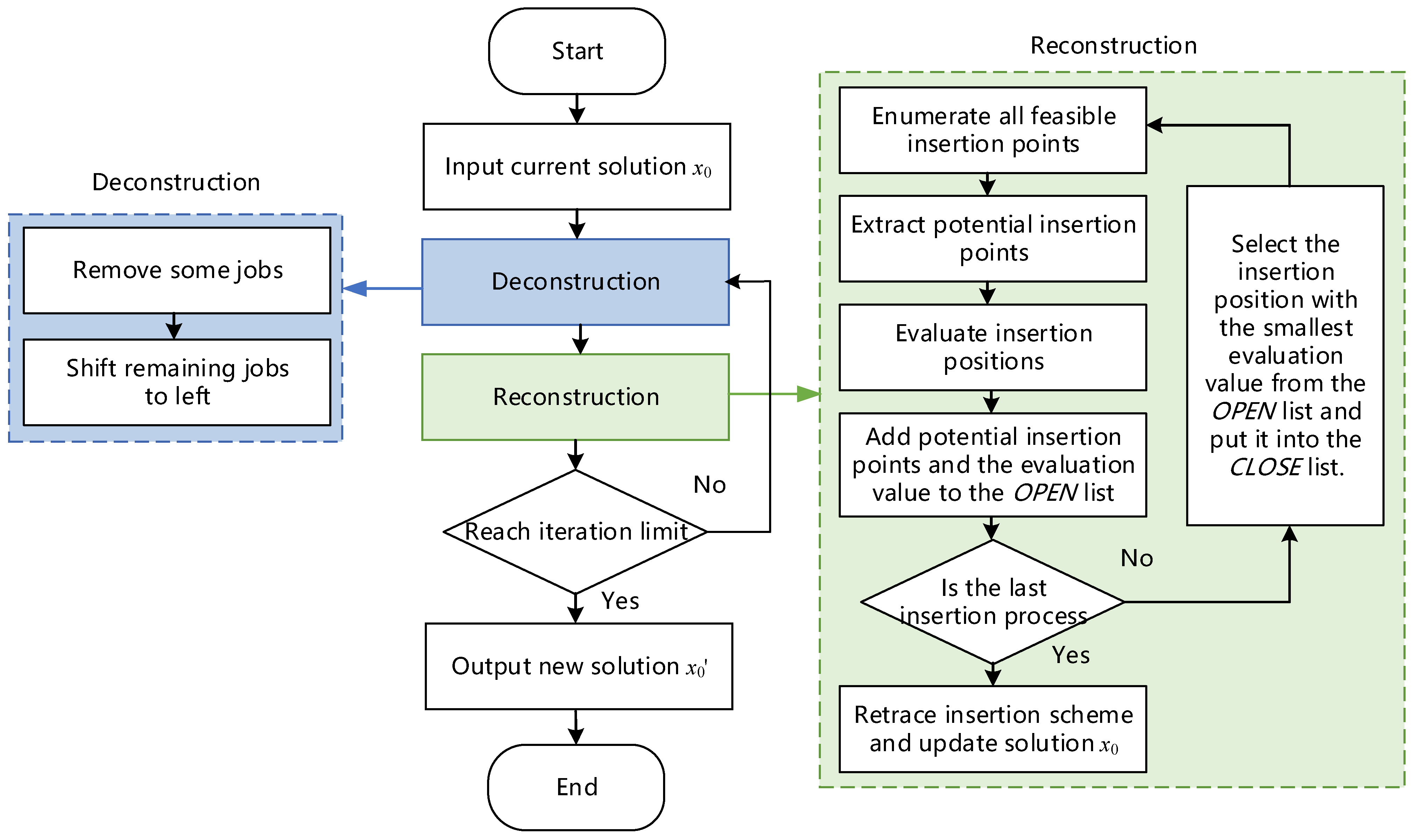
The new job insertion strategy mainly involves two operations of deconstruction and reconstruction. The operation of deconstruction aims to remove some of the currently scheduled jobs, thereby reducing completion time. As for reconstruction, the removed jobs are inserted into the scheduling system successively to obtain a new scheduling scheme. In this paper, a job insertion strategy considering the global optimum is proposed for the HHCFJSP.

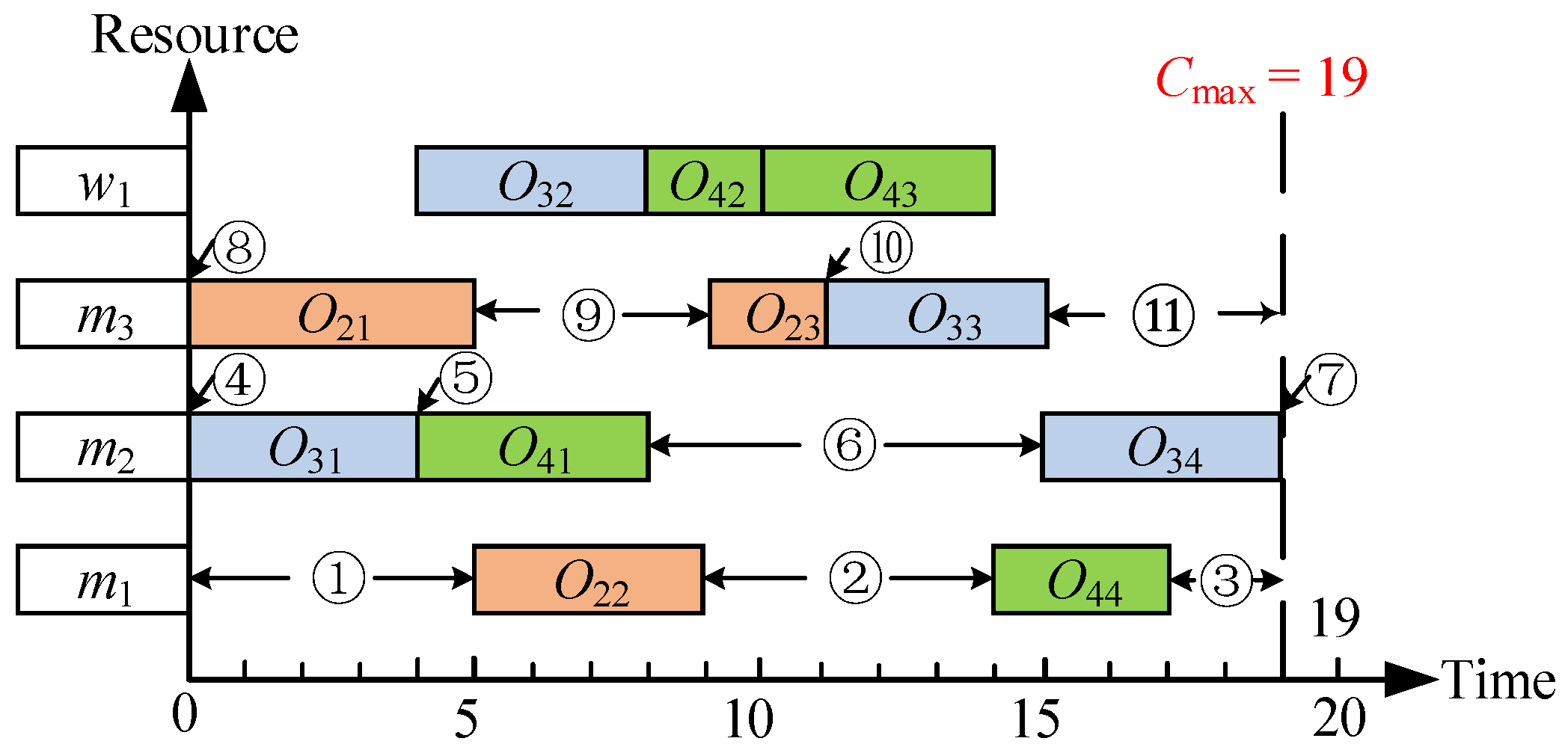
We used the data shown in Figure 2 as an example for deconstruction. As shown in Figure 3, J₁ is removed, and the remaining operations are shifted to the left, reducing C_max from 26 to 19. Next, the job insertion strategy is described in detail.

3.1. Main Framework

Traditional insertion heuristic algorithms commonly adopt the sequence-by-sequence greedy insertion strategy. Only one operation to be scheduled is selected at one time, which is inserted into the current scheduling result, and the scheduling state of the system is instantly updated after each insertion [30]. Although this method is easy to implement and applicable to most heuristic construction processes, it exposes the following two significant drawbacks in complex scheduling problems:

(1)

Obvious trap of local optimization: This strategy only considers the optimal insertion position of the current process at each step and lacks the global consideration of the overall scheduling structure of the jobs. This early optimal decision method will easily lead to the compression of the scheduling space for the remaining operations, making it difficult to insert them reasonably.

(2)

Inefficient utilization of computing resources: Since the processes are inserted one by one, and the scheduling state needs to be reevaluated each time a process is inserted, including the information of resource occupation, priority conflict, etc., the frequent state update significantly increases the computational overhead and affects the overall efficiency of the solution in the case of a large scheduling scale.

In view of this, a job insertion strategy with global optimization search is proposed. Firstly, a bi-objective function is used in conjunction with a non-dominated sorting mechanism to screen potential insertion points. Secondly, an evaluation function is designed to evaluate each potential insertion point. Finally, a heuristic path search method similar to the A* algorithm is introduced to construct a complete insertion scheme. The flow of the proposed job insertion strategy is shown in Figure 4, and the specific steps can be found in Section 3.4. For the proposed strategy, the key techniques involve the selection of operation insertion locations, the design of the evaluation function, and the construction of the insertion scheme, each of which will be described in detail below.

3.2. Selection of Insertion Position

Traditional greedy insertion approaches may seem to be optimal at the early stage of selection, but it will be difficult to insert the remaining processes reasonably due to the compression of the subsequent scheduling space and eventually fall into the local optimum. To solve this problem, this paper introduced a two-dimensional vector evaluation mechanism. The insertion point is jointly evaluated from two dimensions during the insertion process of each operation: (1) Scheduling delay cost G; (2) insertion interval of the remaining processes H.

On the basis of two-dimensional evaluation metrics, the advantages of an insertion point are often characterized by a conflicting relationship between two objectives. For example, one insertion point may greatly compress the scheduling space for subsequent processes although the current delay is minimized. One insertion point, although more flexible, is accompanied by a larger delay cost. At this point, a simple weighted sum method or a single index sort method can easily lead to a bias in favor of one target, masking out the candidate insertion point that has significant advantages in another target. Consequently, this paper introduced a non-dominated sorting mechanism, which maps all candidate insertion points to a two-dimensional target space and identifies solutions that are not simultaneously dominated by other insertion points in both dimensions. This mechanism can effectively retain the potential insertion points that are optimally balanced among a set of objectives, avoiding the distortion of preferences caused by artificial weights, and thus improving the robustness and scalability of the insertion strategy.

Specifically, for each process, all its feasible insertion position segments on the target machine are enumerated. For each insertion point [s, e], the 2D evaluation vector (G, H) is calculated. The set of insertion points satisfying the Pareto frontier is extracted by the non-dominated sorting method and used to construct an A*-like insertion path search structure, which ensures that the insertion strategy achieves a balance between local optimization and global feasibility.

For example, as shown in Figure 5, there are three machines with a total of 11 insertion positions to choose from when O₁₁ is re-inserted into the scheduling scheme. The scheduling cost of O₁₁ and the insertion intervals of the remaining processes are analyzed, and the results are shown in

Table 2. Evaluation of insertion positions.

Operation	No.	Insertion Position	Delay Cost/G	Insertion Interval of Remaining Processes/H	Pareto Front
O11	1	m1[0, 5]	1	[6, 19]/13	√
	2	m1[9, 14]	1	[15, 19]/4	×
	3	m1[17, 19]	4	[23, 19]/−4	×
	4	m2[0, 0]	4	[4, 19]/15	×
	5	m2[4, 4]	4	[8, 19]/11	×
	6	m2[8, 15]	0	[12, 19]/7	×
	7	m2[19, 19]	4	[23, 19]/−4	×
	8	m3[0, 0]	3	[3, 19]/16	√
	9	m3[5, 9]	0	[8, 19]/11	√
	10	m3[11, 11]	3	[14, 19]/5	×
	11	m3[15, 19]	0	[18, 19]/1	×

. We performed a non-dominated sorting method of the results and retained the first level of non-dominated solutions (the set of Pareto fronts) as the potential insertion points. It can be found that three potential insertion locations will be retained, which are locations 1, 8, and 9, and the remaining locations are deleted.

3.3. Design of Evaluation Function

Since the delay distance and the insertion interval of the remaining processes are two independent metrics, an evaluation function is designed in this paper to evaluate the retained potential insertion location, as shown in Equation (2):

$$F_{m_y\left[s,e\right]}^{j,i}=G_{m_y\left[s,e\right]}^{j,i}+H_{m_y\left[s,e\right]}^{j,i}$$

(2)

where $F_{m_y\left[s,e\right]}^{j,i}$ denotes the evaluation value of operation i of job j when the insertion position on machine m_y is [s, e]. $G_{m_y\left[s,e\right]}^{j,i}$ denotes the current scheduling cost. $H_{m_y\left[s,e\right]}^{j,i}$ denotes the minimum delay distance for the remaining processes in the remaining insertion interval.

The calculation of $H_{m_y\left[s,e\right]}^{j,i}$ is shown in Equation (3):

$$H_{m_y\left[s,e\right]}^{j,i}=\left|\min (t_q-t_z,0)\right|$$

(3)

where t_q denotes the length of the insertion interval of remaining processes, and t_z denotes the sum of the minimum processing time of remaining processes.

3.4. Framework of A*-like Insertion Path Search

In order to improve the overall feasibility and consistency of the scheduling solution in the job insertion process, this paper incorporates the heuristic path search idea of the A* algorithm in the minimum-delayed insertion strategy and designs a path construction framework applicable to workpiece-level insertion scheduling. The framework considers each process of a workpiece as a stage node on the path and completes the reasonable insertion of the whole process sequence in the target workshop by gradually expanding the insertion path.

A backtracking mechanism is incorporated to prevent some quality solutions from being missed during the insertion process. Firstly, the first process is scheduled, and the relevant parameters are recorded in the candidate queue. Subsequently, the system continuously selects the insertion position with the optimal evaluation index from the queue to guide the arrangement of the subsequent processes. The algorithm terminates and outputs the globally optimal scheduling scheme when the last process is successfully placed. The specific steps are shown below:

Step1: Input information. The job j = {O_j,1, …, O_j,i, …, O_j,n} to be inserted and the existing scheduling scheme are known.

Step2: Initialize the insertion processes. The details are as follows:

(1)

For the first process O_j,1, enumerate all feasible insertion points.

(2)

Calculate the 2D evaluation vector (G, H) for each insertion point.

(3)

Perform non-dominated sorting to extract potential insertion points.

(4)

Evaluate each potential insertion point with the evaluation function f_delay.

(5)

Add the potential insertion points as well as the evaluation value to the OPEN list.

Step3: Circulate insertion process. The details are as follows:

(1)

Select the insertion position information with currently minimum f_delay from the OPEN list and move it into the CLOSE list.

(2)

If the insertion position information is generated by the final process, skip to step 4. Otherwise, perform insertion for the next process O_j,i+1 (in a similar way to step 2).

(3)

Add the potential insertion points for O_j,i+1 as well as the evaluation value to the OPEN list.

Step4: Backtrack insertion scheme. Backtrack sequentially from the last process to the first process and record the insertion positions of all processes.

Step5: Update. Perform the insertion operation in the backtracking path to insert all the processes into the scheduling solution in sequence.

To visualize the search process, we continue to take the insertion of j₁ = {O₁₁, O₁₂, O₁₃, O₁₄} as an example. For the first process O₁₁, all its feasible insertion points are shown in Figure 5. We calculate the 2D evaluation vector (G, H) for each point and obtain three potential insertion points after non-dominated sorting of the results (as shown in Table 2). Then we calculate the evaluation value of the 3 potential insertion points according to the evaluation function f_delay in Equation (2). The potential insertion points as well as the evaluation value are added to the OPEN list. The information of the insertion position with current minimum f_delay is selected from the OPEN list and added into the CLOSE list.

After the first search, the OPEN list and the CLOSE list are shown in

Table 3. The OPEN list and CLOSE list after the first search.

OPEN List
Operation	Insertion position	Evaluation value
O11	m1[0, 5]	1
	m3[0, 0]	3
	m3[5, 9]	0
CLOSE List
Operation	Insertion position	Evaluation value
O11	m3[5, 9]	0

. O_{11_}m₃[5, 9], which has the smallest evaluation value in the OPEN list, is selected to be removed from the OPEN list and added to the CLOSE list.

After the second search, the OPEN list and the CLOSE list are shown in

Table 4. The OPEN list and CLOSE list after the second search.

OPEN List
Operation	Insertion position	Evaluation value
O11	m1[0, 5]	1
	m3[0, 0]	3
O12	m4[8, 8]	3
	w1[14, 19]	2
CLOSE List
Operation	Insertion position	Evaluation value
O11	m3[5, 9]	0
	m1[0, 5]	1

. O_{11_}m₁[0, 5], which has the smallest evaluation value in the OPEN list, is selected to be removed from the OPEN list and added to the CLOSE list.

We circulate the above operations until the last process is inserted.

Table 5. Insertion process of job 1.

Search Number	Operation	Insertion Position	Insertion Interval of Remaining Processes	Evaluation Value
				G	H	F
1	O11	m1[0, 5]	[6, 19]/13	1	0	1
		m3[0, 0]	[3, 19]/16	3	0	3
		m3[5, 9]	[8, 19]/11	0	0	0
Select O11_m3[5, 9] and guide the insertion of next process
2	O12	w1[8, 8]	[11, 19]/8	3	0	3
		w1[14, 19]	[17, 19]/2	0	2	2
Select O11_m1[0, 5] and guide the insertion of next process
3	O12	m3[6, 9]	[10, 19]/9	1	0	1
Select O12_m3[6, 9] and guide the insertion of next process
4	O13	m2[10, 15]	[13, 19]/6	0	0	0
		m3[10, 10]	[12, 19]/7	2	0	2
Select O13_m2[10, 15] and guide the insertion of next process
5	O14	w1[14, 19]	[16, 19]/3	0	0	0
Select O14_w1[14, 19] and end the insertion

shows the full process of reinserting job 1 into the scheduling plan. After the 5th search, the search ends because the last process O₁₄ is included. The optimal insertion scheme O_{11_}m₁[0, 5] → O_{12_}m₃[6, 9] → O_{13_}m₂[10, 15] → O_{14_}w₁[14, 19] is backtracked in the CLOSE list, and the insertion positions are shown in Figure 6a. The scheduling scheme is re-decoded after the insertion is completed. As shown in Figure 6b, the maximum completion time is reduced from 26 to 20 because the insertion position with the smallest total delay is selected for each process.

4. Two-Stage Job Insertion Algorithm

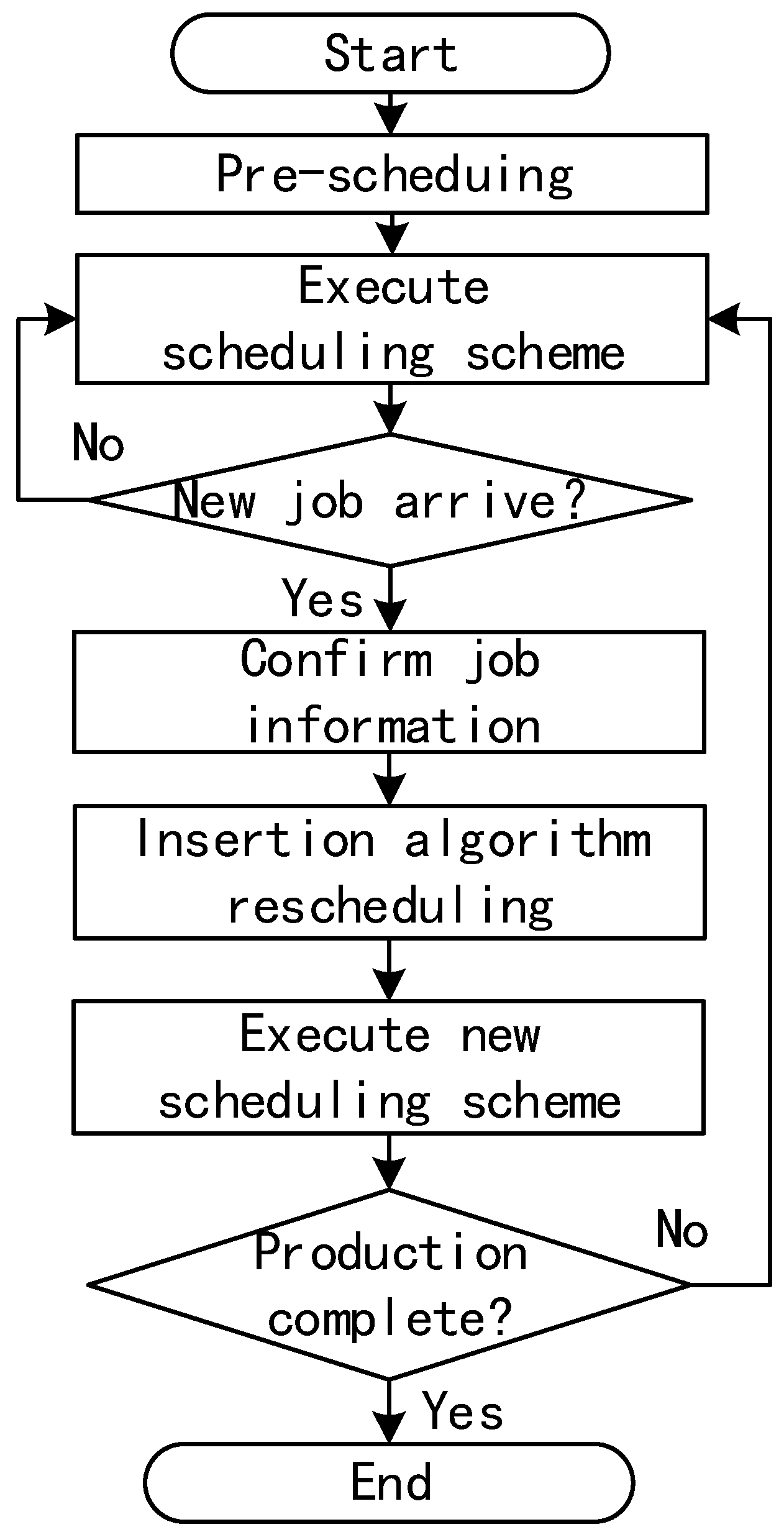
Prior to the execution of production planning, the workshop must perform pre-scheduling. Pre-scheduling is essential to ensure the smoothness of the production process and helps to avoid production delays and quality degradation due to resource shortages. Therefore, this paper adopts two-stage scheduling. We first complete the static scheduling of pre-scheduling. Then, on the basis of pre-scheduling, we do the re-scheduling operations in the face of the random job arrivals dynamically. The process framework is shown in Figure 7.

4.1. Pre-Scheduling

In the pre-scheduling phase, this section will introduce a hybrid algorithm based on improved job insertion strategy (HAIJI), as shown in Algorithm 1. Firstly, the job insertion algorithm is used to perturb the scheduling scheme globally and adjust the machining order and machine allocation of key jobs dynamically. Subsequently, the tabu search algorithm is used to make local adjustments. Thus, the balance in global as well as local search is realized.

Algorithm 1 Pseudo-code for HAIJI
	Input: the problem information, including workpiece information, machine information, process routing, etc.
	Output: the best solution xb
1:	Set algorithm parameters, iter = 0, maximum number of iterations Maxiter = 300
2:	Generate an initial solution x0, complete time f(x0), current solution xc ← x0, best solution xb ← x0
3:	While (iter <= Maxiter) do
4:	For j = {1, 2, …, n}                      //j-th job in the workshop
5:	(j, x0′) ← Deconstruction (x0)         //remove j, remaining scheduling x0′
6:	πj = Reconstruction (j, x0′)         //job insertion algorithm
7:	End For                            //neighborhood solution set π = {π1, π2, …, πn}
8:	For i = {1, 2, …, n}                      //local search
9:	Πi ← Tabu Search (πi)
10:	End For                                       //Π = {Π1, Π2, …, Πn}
11:	xb′ ← Select the best solution among (Π∪π)
12:	If f(xb′) < f(xb)
13:	xb ← xb′, xc ← xb
14:	Else
15:	xc ← Randomly select a solution from Π
16:	End if
17:	iter = iter + 1
18:	End While
19:	Return xb

4.1.1. Encoding, Decoding and Initial Solution

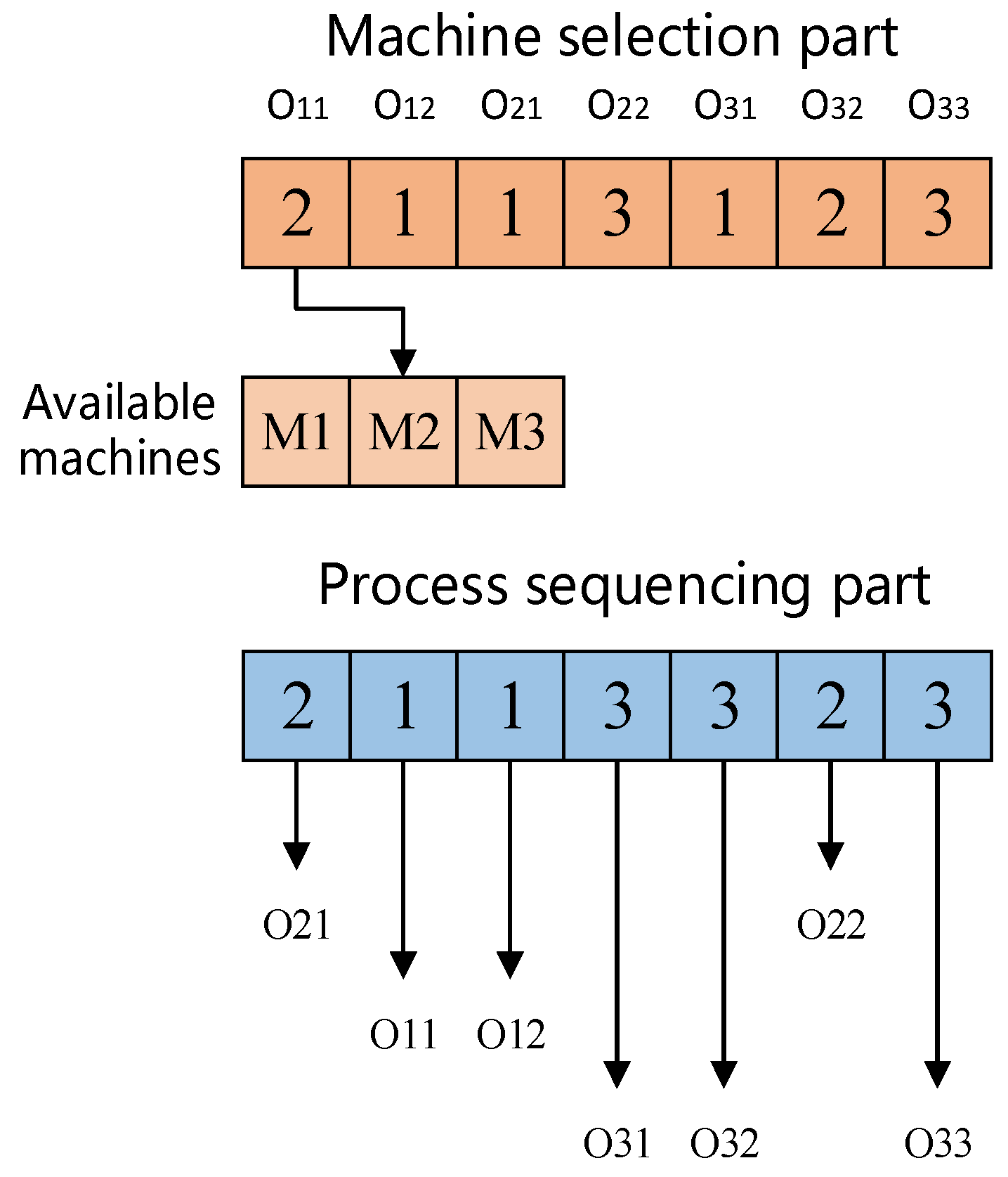
There are two main issues to consider when encoding: machine selection and process sequencing. In this paper, segmented integer encoding is used to define the feasible solution, as shown in Figure 8. The machine selection part is responsible for solving the problem of which machine each operation is processed on. The process sequencing part is responsible for solving the problem of ordering all processes. The value at each position represents the job index, which indicates the first process of the job when it appears for the first time, the second process when it appears for the second time, and so on. Decoding is done in a semi-active way, i.e., the processes on the code are processed from left to right according to the earliest start time.

It is found that the initial solution will not have a big impact on the final result of the pre-scheduling. Meanwhile, the pre-scheduling does not have strict requirements on the running time. Thus, this paper adopts a randomized generation of the initial solution, i.e., the order of the process and the selection of the machine are randomized.

4.1.2. Job Insertion Algorithm

The job insertion algorithm is the core optimization method in the pre-scheduling phase, aiming at reducing the total completion time by dynamically adjusting the machining sequence and machine allocation of the processes and gradually optimizing the initial scheduling solution. The algorithm deconstructs and reconstructs each critical job in the current solution. The deconstruction and reconstruction phases make the scheduling scheme progressively approximate a more optimal solution by iteratively removing and reinserting critical jobs.

In the deconstruction phase, the algorithm first identifies the critical job in the current scheduling solution. Critical jobs contain critical processes, which constitute the longest machining path (i.e., the process chain that has the greatest impact on makespan). The specific steps are as follows: Removing critical job: Temporarily remove the selected the critical job from the current scheduling scheme while leaving the machine allocation and the machining sequence of the other jobs unchanged. Shifting the remaining processes to the left: Shift the remaining processes to the left without changing the process order to shorten the idle time and thus reduce the temporary makespan.

In the reconfiguration phase, the algorithm reinserts the removed critical job into the left-shift scheduling scheme using the job insertion algorithm.

The algorithm progressively optimizes the scheduling scheme by executing the deconstruction and reconstruction phases several times. In each iteration, the removal and reinsertion of critical jobs leads to a potential improvement in makespan. When a predefined number of iterations is reached or makespan is no longer significantly improved, the algorithm terminates and outputs the final pre-scheduling solution.

4.1.3. Local Search

Since the job insertion algorithm is a large change in scheduling optimization, it is necessary to use local search to improve the solution. Tabu search combined with the designed neighborhood structure will have a powerful local search capability. In the hybrid algorithm, Tabu search performs a local search only on the neighborhood solution generated by the job insertion algorithm. The process generates neighborhood solutions by the neighborhood structure for each neighborhood solution π_i. To avoid falling into a local optimum, a tabu list is used to tabu the solutions that have already been searched. In the hybrid algorithm, the N7 [31] and Nk [32] neighborhood structures are used to generate a neighborhood solution, and an approximate evaluation method [33] is used to evaluate the neighborhood solution. Other components, including the tabu table, amnesty criterion, move attribute, and termination criteria, can be found in the literature [31].

4.2. Random Job Arrival

The scheduling system must react quickly after the disturbance occurs to maintain smooth execution of production on the shop floor. Dynamic rescheduling strategies are generally categorized into event-driven and cycle-driven. Event-driven rescheduling means that the rescheduling strategy is carried out immediately when a dynamic event occurs in the work shop. Cycle-driven rescheduling means that the rescheduling detection is carried out at intervals in the work shop, no matter whether there is a dynamic disturbance or not. Event-driven rescheduling has good real-time performance and minimizes the impact of disturbance events on production and processing. Therefore, an event-driven rescheduling strategy is used in this paper.

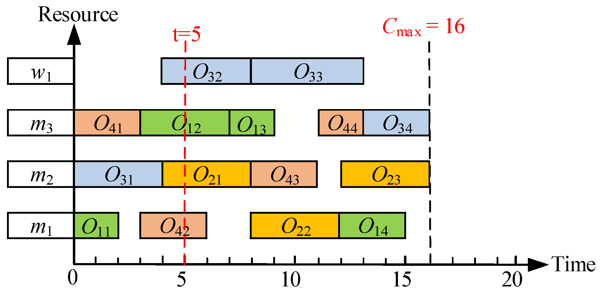
When a new job arrives at a certain time, insertion rescheduling is performed using the job insertion algorithm proposed in this paper. Taking Figure 9 as an example, at t = 5, the new job J₅ arrives. The machines selected for each process as well as the processing time are shown in

Table 6. Information of job 5 to be inserted.

Job	Operation	Available Resources and Processing Time
		M1	M2	M3	W1
Job 5	O5,1	-	4	-	3
	O5,2	-	3	3	-
	O5,3	-	3	2	3

. At this time, the processes in the scheduling plan can be divided into three categories: been processed, being processed, and to be processed. We keep the processes that have been processed and those that are being processed unchanged on the left side of the dotted line and on the dotted line. The new processes are inserted between the processes that are to be processed on the right side of the dotted line.

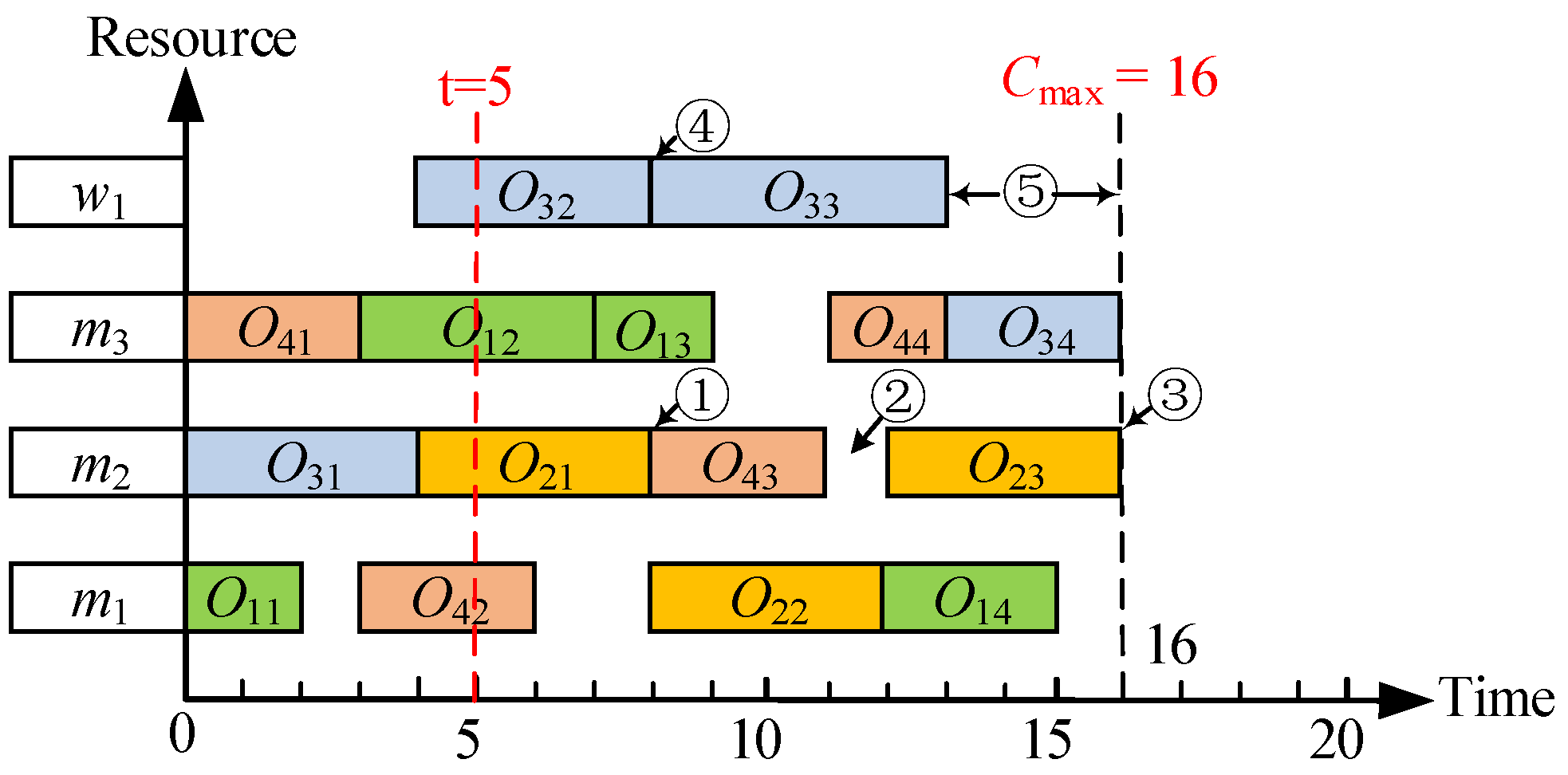
Take the insertion of O₅₁ as an example; O₅₁ can be processed on M₂ or W₁. After the arrival time, we select all interval between the processes that are to be processed as candidate insertion points. As shown in Figure 10, there are 5 candidate insertion points on the right side of the dotted line. We calculate the 2D evaluation vector (G, H) of each point and get 1 potential insertion point w₁[8, 8] after non-dominated sorting of the result. We insert the remaining 2 processes and finally get the insertion scheme: w₁[8, 8] → m₂[11, 16] → w₁[16, 19]. As shown in Figure 11, the scheduling scheme with a makespan of 19 is finally obtained.

Table 7. Insertion process of job 5.

Search Number	Operation	Insertion Position	Insertion Interval of Remaining Processes	Evaluation Value
				G	H	F
1	O51	w1[8, 8]	[11, 16]/5	3	0	3
Select O51_w1[8, 8] and guide the insertion of next process
2	O52	m2[11, 12]	[14, 16]/2	2	0	2
Select O52_m2[11, 12] and guide the insertion of next process
3	O53	w1[14, 16]	[17, 16]/-1	1	1	2
Select O53_w1[14, 19] and end the insertion

demonstrates the process of the job insertion algorithm to insert the newly arrived J₅ into the pre-scheduled schedule.

5. Experimental Studies and Results

In order to verify the effectiveness of the job insertion algorithm for random job arrival events in a flexible job shop environment, this paper carries out simulation experiments of two-stage scheduling and analyzes the experimental results in detail. The algorithms in this paper are implemented using MATLAB R2023b programming on a test computer with a CPU of 3.40 GHz and 32 GB of RAM.

5.1. Test of Pre-Scheduling

In this paper, 10 Brandimarte benchmark instances as well as 21 BCdata benchmark instances are taken as test instances for experiments. Each instance is tested 20 times, and the results are shown in

Table 8. The solution results of the Brandimarte example and the BCdata example.

Problem	n × m	LB	Proposed Algorithm
			Cmax	AV (Cmax)	AV (CPU)	RE
mk01	10 × 6	36	40	40.00	0.76	11.11
mk02	10 × 6	24	26	26.15	1.77	8.33
mk03	15 × 8	204	204	204.00	2.84	0.00
mk04	15 × 8	48	60	60.45	1.34	25.00
mk05	15 × 4	168	172	172.95	2.13	2.38
mk06	10 × 15	33	57	58.55	9.48	72.73
mk07	20 × 5	133	139	139.50	1.78	4.51
mk08	20 × 10	523	523	523.00	5.41	0.00
mk09	20 × 10	299	307	307.15	10.08	2.68
mk10	20 × 15	165	198	201.75	23.48	20.00
mt10c1	10 × 11	655	927	928.45	2.70	41.53
mt10cc	10 × 12	655	910	912.70	2.17	38.93
mt10x	10 × 11	655	918	919.70	2.07	40.15
mt10xx	10 × 12	655	918	918.55	1.77	40.15
mt10xxx	10 × 13	655	918	918.10	1.82	40.15
mt10xy	10 × 12	655	905	906.25	1.78	38.17
mt10xyz	10 × 13	655	847	858.50	1.67	29.31
setb4c9	15 × 11	857	914	920.65	3.69	6.65
setb4cc	15 × 12	857	908	913.35	3.37	5.95
setb4x	15 × 11	846	925	934.35	2.85	9.34
setb4xx	15 × 12	846	925	933.55	2.31	9.34
setb4xxx	15 × 13	846	925	933.85	3.03	9.34
setb4xy	15 × 12	845	911	922.70	2.38	7.81
setb4xyz	15 × 13	838	905	913.95	2.18	8.00
seti5c12	15 × 16	1027	1174	1185.10	4.69	14.31
seti5cc	15 × 17	955	1136	1146.30	4.56	18.95
seti5x	15 × 16	955	1200	1212.95	5.09	25.65
seti5xx	15 × 17	955	1199	1205.60	6.22	25.55
seti5xxx	15 × 18	955	1198	1206.90	4.59	25.45
seti5xy	15 × 17	955	1136	1146.20	4.62	18.95
seti5xyz	15 × 18	955	1127	1133.90	4.44	18.01

, where n × m denotes that there are n jobs and m machines in the instance, LB denotes the lower bound of the optimal solution, C_maxdenotes the optimal maximum completion time, AV (C_max) denotes the average value of the optimal maximum completion time, AV (CPU) denotes the average time spent in each time of solving for the optimal maximum completion time, and RE denotes the relative deviation of C_max from LB. MRE is the mean value of RE and can be used to comparatively measure the overall performance of different algorithms.

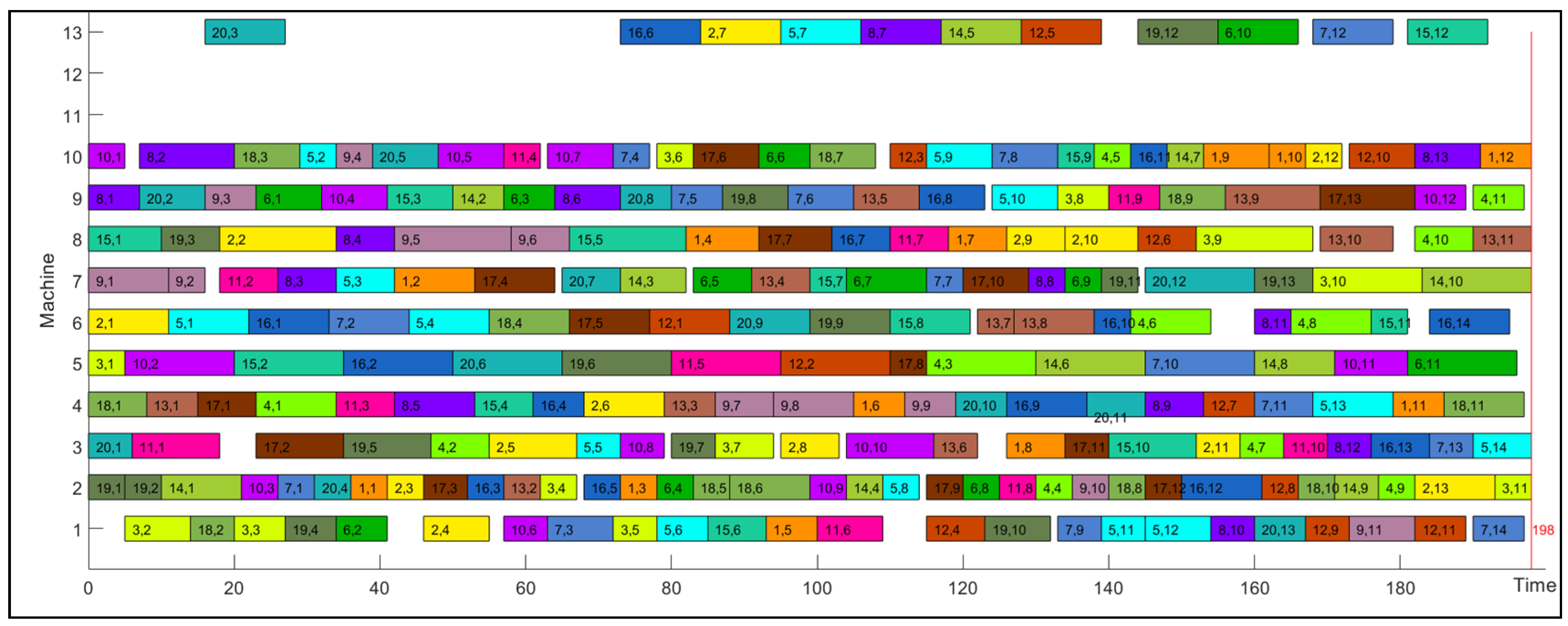
The test results of the Brandimarte instances were compared with three comparison algorithms, namely hGA [34], CDDS [35], and BEDA [36]. As shown in

Table 9. Comparative analysis of HAIJI and other algorithms in solving Brandimarte instances.

Problem	LB	hGA		CDDS		BEDA		Ours
		Cmax	RE	Cmax	RE	Cmax	RE	Cmax	RE
mk01	36	40	11.11	40	11.11	40	11.11	40	11.11
mk02	24	26	8.33	26	8.33	26	8.33	26	8.33
mk03	204	204	0	204	0	204	0	204	0
mk04	48	60	25.00	60	25.00	60	25.00	60	25.00
mk05	168	172	2.38	173	4.17	172	2.98	172	2.38
mk06	33	58	75.76	58	96.97	60	90.91	57	72.73
mk07	133	139	4.51	139	9.02	139	7.52	139	4.51
mk08	523	523	0	523	0	523	0	523	0
mk09	299	307	2.68	307	2.68	307	2.68	307	2.68
mk10	165	199	20.61	210	30.30	206	27.27	198	20.00
MRE	-	-	15.04	-	18.76	-	17.58	-	14.67

, our algorithm achieves better solutions than the comparison algorithms on mk06 and mk10. For the mk06, the three comparison algorithms obtained the C_maxof hGA (58), CDDS (58), and BEDA (60). The algorithm in this paper optimized C_maxto 57. For the mk10, the three comparison algorithms obtained the C_maxof hGA (199), CDDS (210), and BEDA (206). The algorithm in this paper optimized C_maxto 198. The Gantt chart for the mk10 case obtained by our algorithm is given in Figure 12. In addition, the MRE of our algorithm is 14.67, which is lower than that of hGA (15.04), CDDS (18.76), and BEDA (17.58).

The test results of the BCdata instances were compared with three comparison algorithms, namely hGA [35], eGA [37], and TSBM²H [38]. As shown in

Table 10. Comparative analysis of HAIJI and other algorithms in solving BCdata instances.

Problem	LB	hGA		eGA		TSBM2H		Ours
		Cmax	RE	Cmax	RE	Cmax	RE	Cmax	RE
mt10c1	655	927	41.53	927	41.53	927	41.53	927	41.53
mt10cc	655	910	38.93	910	38.93	908	38.63	910	38.93
mt10x	655	918	40.15	918	40.15	922	40.76	918	40.15
mt10xx	655	918	40.15	918	40.15	918	40.15	918	40.15
mt10xxx	655	918	40.15	918	40.15	918	40.15	918	40.15
mt10xy	655	905	38.17	905	38.17	905	38.17	905	38.17
mt10xyz	655	849	29.62	847	29.31	849	29.31	847	29.31
setb4c9	857	914	6.65	914	6.65	914	6.65	914	6.65
setb4cc	857	914	6.65	909	6.07	909	6.07	908	5.95
setb4x	846	925	9.34	925	9.34	925	9.34	925	9.34
setb4xx	846	925	9.34	925	9.34	925	9.34	925	9.34
setb4xxx	846	925	9.34	925	9.34	925	9.34	925	9.34
setb4xy	845	916	8.40	916	7.93	912	7.93	911	7.81
setb4xyz	838	905	8.00	905	8.00	903	8.00	905	8.00
seti5c12	1027	1175	14.41	1174	14.31	1174	14.31	1174	14.31
seti5cc	955	1138	19.16	1136	18.95	1136	18.95	1136	18.95
seti5x	955	1204	26.07	1209	25.65	1198	26.07	1200	25.65
seti5xx	955	1202	25.86	1204	25.45	1197	25.65	1199	25.55
seti5xxx	955	1204	26.07	1204	25.45	1197	25.55	1198	25.45
seti5xy	955	1136	18.95	1136	18.95	1136	18.95	1136	18.95
seti5xyz	955	1126	17.91	1125	18.01	1128	18.01	1127	18.01
MRE	-	-	22.61	-	22.47	-	22.52	-	22.46

, our algorithm achieves better solutions than the comparison algorithms on setb4cc and setb4xy. For the setb4cc, the three comparison algorithms obtained the C_maxof hGA (914), eGA (909), and TSBM²H (909). The algorithm in this paper optimized C_maxto 908. For the setb4xy, the three comparison algorithms obtained the C_maxof hGA (916), eGA (916), and TSBM²H (912). The algorithm in this paper optimized C_maxto 911. In addition, the MRE of our algorithm is 22.46, which is lower than that of hGA (22.61), eGA (22.47), and TSBM²H (22.52).

5.2. Test of Random Job Arrival

To verify the effectiveness of the job insertion algorithm in solving the random job arrival problem, this paper deals with the random job arrival events with the objective of minimizing the completion time. The initial scheduling scheme Gantt chart is shown in Figure 13. Assuming that a new job J₁₁ arrives at the time t = 20, the information of this job is shown in

Table 11. Information of job 11 to be inserted.

Job	Operation	Available Resources and Processing Time
		M1	M2	M3	M4	W1	W2
Job 11	O11,1	-	6	-	-	-	-
	O11,2	-	-	4	2	-	6
	O11,3	1	6	-	5	-	-
	O11,4	-	6	4	6	-	8
	O11,5	1	-	-	-	5	-

. In this case, as shown in Figure 14, the completion time of 53 is obtained using the right-shift rescheduling method. As shown in Figure 15, the completion time of 47 is obtained using the job insertion algorithm proposed in this paper.

According to the simulation experiments in Figure 14 and Figure 15, it is shown that when random job arrival events occur, the job insertion algorithm is able to maintain the stability of the scheduling scheme and achieve the desirable completion time while changing the original scheme by only a small margin.

To further verify the impact of the job insertion algorithm on the current scheduling scheme when inserting new jobs, the Delay Rate (DR) is introduced as shown in Equation (4):

$$DR={\displaystyle \frac{{C_{\max }}^{\prime }-C_{\max }}{{C_{\max }}^{\prime }}}\times 100\%$$

(4)

where C_maxdenotes the maximal completion time for static scheduling and C_max′ denotes the maximal completion time after re-scheduling. The smaller the DR is, the smaller the impact on the maximal completion time is caused by the arrival of new jobs. MDR denotes the mean delay rate.

Take Brandimarte instances (mk01–mk10) as test instances. After pre-scheduling, the jobs are simulated to arrive randomly, where the random arrival time t is uniformly distributed in [1, C_max]. The randomized jobs are the randomized jobs in the current instance. We performed 20 simulation experiments with the right-shift rescheduling method and the proposed algorithm, respectively, on each instance and counted the average delay rate. The results are shown in

Table 12. Delay rate.

Problem	Right-Shift Rescheduling	Proposed Algorithm
mk01	12.32%	2.15%
mk02	15.14%	2.06%
mk03	20.56%	5.21%
mk04	19.83%	4.78%
mk05	21.73%	5.06%
mk06	20.86%	6.73%
mk07	23.76%	6.48%
mk08	25.35%	9.79%
mk09	18.91%	10.74%
mk10	16.68%	10.31%
MDR	19.51%	6.33%

. In all 10 benchmark instances, the MDR of the proposed algorithm is significantly better than that of the traditional right-shift rescheduling method. The proposed algorithm possesses better stability. Meanwhile, the solving time of the proposed algorithm is less than 0.1 s each time, which reflects the extremely fast response speed.

6. Conclusions

In this paper, an efficient job insertion algorithm is proposed for the hybrid human–machine collaborative flexible job shop scheduling problem with random job arrivals. The proposed algorithm filters potential insertion points through a bi-objective evaluation function and a non-dominated sorting mechanism. It combines the A*-like heuristic path search framework to achieve the global balance between the scheduling delay cost and the remaining job insertion space when inserting new jobs, which effectively avoids the local optimal traps of the traditional greedy insertion strategy. The two-stage scheduling framework (pre-scheduling static scheduling and dynamic re-scheduling) is used to optimize the initial scheduling scheme with taboo search in the pre-scheduling stage and to respond to random job arrivals quickly with the event-driven strategy in the dynamic re-scheduling stage, which takes into account the stability of the production system and the quality of the scheduling. Experiments show that the proposed algorithm is able to obtain a shorter maximum completion time under static scheduling. While under dynamic scheduling, it can significantly reduce the maximum completion time with only a small change to the original scheduling scheme, which improves the equipment utilization rate and system response speed.

This paper delves into the impact of HAIJI on production efficiency within a human–machine collaborative production model, offering practical guidance for real-world applications. However, the human–machine collaboration model examined in this study is limited to single-worker, single-machine scenarios and does not account for more complex collaborative modes. In real production there are workshops with different production functions. Therefore, we will use HAIJI to solve the more complex workshop scheduling problems.

References

1. Zhou, J.; Li, P.; Zhou, Y.; Wang, B.; Zang, J.; Meng, L. Toward New-Generation Intelligent Manufacturing. Engineering 2018, 4, 11–20. [Google Scholar] [CrossRef]
2. Zhou, J.; Zhou, Y.; Wang, B.; Zang, J. Human–Cyber–Physical Systems (HCPSs) in the Context of New-Generation Intelligent Manufacturing. Engineering 2019, 5, 624–636. [Google Scholar] [CrossRef]
3. Lu, C.; Gao, R.; Yin, L.; Zhang, B. Human–Robot Collaborative Scheduling in Energy-Efficient Welding Shop. IEEE Trans. Ind. Inform. 2024, 20, 963–971. [Google Scholar] [CrossRef]
4. Geng, K.; Ye, C.; Liu, L. Research on Multi-Objective Hybrid Flow Shop Scheduling Problem With Dual Resource Constraints Using Improved Memetic Algorithm. IEEE Access 2020, 8, 104527–104542. [Google Scholar] [CrossRef]
5. Ferreira, C.; Figueira, G.; Amorim, P. Scheduling Human-Robot Teams in Collaborative Working Cells. Int. J. Prod. Econ. 2021, 235, 108094. [Google Scholar] [CrossRef]
6. Wu, Y.; Wang, L.; Li, R.; Chen, J. A Reinforcement Learning-Driven Adaptive Decomposition Algorithm for Multi-Objective Hybrid Seru System Scheduling Considering Worker Transfer. Swarm Evol. Comput. 2024, 88, 101602. [Google Scholar] [CrossRef]
7. Usman, S.; Lu, C. Job-Shop Scheduling with Limited Flexible Workers Considering Ergonomic Factors Using an Improved Multi-Objective Discrete Jaya Algorithm. Comput. Oper. Res. 2024, 162, 106456. [Google Scholar] [CrossRef]
8. Song, H.; Li, J.; Du, Z.; Yu, X.; Xu, Y.; Zheng, Z.; Li, J. A Q-Learning Driven Multi-Objective Evolutionary Algorithm for Worker Fatigue Dual-Resource-Constrained Distributed Hybrid Flow Shop. Comput. Oper. Res. 2025, 175, 106919. [Google Scholar] [CrossRef]
9. Bouaziz, N.; Bettayeb, B.; Sahnoun, M.; Yassine, A. Incorporating Uncertain Human Behavior in Production Scheduling for Enhanced Productivity in Industry 5.0 Context. Int. J. Prod. Econ. 2024, 274, 109311. [Google Scholar] [CrossRef]
10. Rahman, H.F.; Servranckx, T.; Chakrabortty, R.K.; Vanhoucke, M.; El Sawah, S. Manufacturing Project Scheduling Considering Human Factors to Minimize Total Cost and Carbon Footprints. Appl. Soft Comput. 2022, 131, 109764. [Google Scholar] [CrossRef]
11. Berti, N.; Finco, S.; Battaïa, O.; Delorme, X. Ageing Workforce Effects in Dual-Resource Constrained Job-Shop Scheduling. Int. J. Prod. Econ. 2021, 237, 108151. [Google Scholar] [CrossRef]
12. Gao, K.Z.; Suganthan, P.N.; Chua, T.J.; Chong, C.S.; Cai, T.X.; Pan, Q.K. A Two-Stage Artificial Bee Colony Algorithm Scheduling Flexible Job-Shop Scheduling Problem with New Job Insertion. Expert Syst. Appl. 2015, 42, 7652–7663. [Google Scholar] [CrossRef]
13. Fan, J.; Zhang, C.; Liu, Q.; Shen, W.; Gao, L. An Improved Genetic Algorithm for Flexible Job Shop Scheduling Problem Considering Reconfigurable Machine Tools with Limited Auxiliary Modules. J. Manuf. Syst. 2022, 62, 650–667. [Google Scholar] [CrossRef]
14. Liu, M.; Liu, X.; Chu, F.; Zhang, E.; Chu, C. Service-Oriented Robust Worker Scheduling with Motivation Effects. Int. J. Prod. Res. 2021, 59, 2328–2351. [Google Scholar] [CrossRef]
15. Lou, H.; Wang, X.; Dong, Z.; Yang, Y. Memetic Algorithm Based on Learning and Decomposition for Multiobjective Flexible Job Shop Scheduling Considering Human Factors. Swarm Evol. Comput. 2022, 75, 101204. [Google Scholar] [CrossRef]
16. Shi, J.; Chen, M.; Ma, Y.; Qiao, F. A New Boredom-Aware Dual-Resource Constrained Flexible Job Shop Scheduling Problem Using a Two-Stage Multi-Objective Particle Swarm Optimization Algorithm. Inf. Sci. 2023, 643, 119141. [Google Scholar] [CrossRef]
17. Destouet, C.; Tlahig, H.; Bettayeb, B.; Mazari, B. Multi-Objective Sustainable Flexible Job Shop Scheduling Problem: Balancing Economic, Ecological, and Social Criteria. Comput. Ind. Eng. 2024, 195, 110419. [Google Scholar] [CrossRef]
18. Vital-Soto, A.; Baki, M.F.; Azab, A. A Multi-Objective Mathematical Model and Evolutionary Algorithm for the Dual-Resource Flexible Job-Shop Scheduling Problem with Sequencing Flexibility. Flex. Serv. Manuf. J. 2023, 35, 626–668. [Google Scholar] [CrossRef]
19. Teng, G. An Improved Genetic Algorithm for Dual-Resource Constrained Flexible Job Shop Scheduling Problem with Tool-Switching Dependent Setup Time. Expert Syst. Appl. 2025, 281, 127496. [Google Scholar] [CrossRef]
20. Barak, S.; Javanmard, S.; Moghdani, R. Dual Resource Constrained Flexible Job Shop Scheduling with Sequence-Dependent Setup Time. Expert Syst. 2024, 41, e13669. [Google Scholar] [CrossRef]
21. Gao, K.Z.; Suganthan, P.N.; Tasgetiren, M.F.; Pan, Q.K.; Sun, Q.Q. Effective Ensembles of Heuristics for Scheduling Flexible Job Shop Problem with New Job Insertion. Comput. Ind. Eng. 2015, 90, 107–117. [Google Scholar] [CrossRef]
22. Zakaria, Z.; Petrovic, S. Genetic Algorithms for Match-up Rescheduling of the Flexible Manufacturing Systems. Comput. Ind. Eng. 2012, 62, 670–686. [Google Scholar] [CrossRef]
23. Li, X.; Peng, Z.; Du, B.; Guo, J.; Xu, W.; Zhuang, K. Hybrid Artificial Bee Colony Algorithm with a Rescheduling Strategy for Solving Flexible Job Shop Scheduling Problems. Comput. Ind. Eng. 2017, 113, 10–26. [Google Scholar] [CrossRef]
24. Zhang, L.; Gao, L.; Li, X. A Hybrid Genetic Algorithm and Tabu Search for a Multi-Objective Dynamic Job Shop Scheduling Problem. Int. J. Prod. Res. 2013, 51, 3516–3531. [Google Scholar] [CrossRef]
25. Luo, S. Dynamic Scheduling for Flexible Job Shop with New Job Insertions by Deep Reinforcement Learning. Appl. Soft Comput. 2020, 91, 106208. [Google Scholar] [CrossRef]
26. Zhao, L.; Fan, J.; Zhang, C.; Shen, W.; Zhuang, J. A DRL-Based Reactive Scheduling Policy for Flexible Job Shops With Random Job Arrivals. IEEE Trans. Autom. Sci. Eng. 2024, 21, 2912–2923. [Google Scholar] [CrossRef]
27. Lei, K.; Guo, P.; Wang, Y.; Zhang, J.; Meng, X.; Qian, L. Large-Scale Dynamic Scheduling for Flexible Job-Shop With Random Arrivals of New Jobs by Hierarchical Reinforcement Learning. IEEE Trans. Ind. Inform. 2024, 20, 1007–1018. [Google Scholar] [CrossRef]
28. Lu, S.; Wang, Y.; Kong, M.; Wang, W.; Tan, W.; Song, Y. A Double Deep Q-Network Framework for a Flexible Job Shop Scheduling Problem with Dynamic Job Arrivals and Urgent Job Insertions. Eng. Appl. Artif. Intell. 2024, 133, 108487. [Google Scholar] [CrossRef]
29. Xu, S.; Li, Y.; Li, Q. A Deep Reinforcement Learning Method Based on a Transformer Model for the Flexible Job Shop Scheduling Problem. Electronics 2024, 13, 3696. [Google Scholar] [CrossRef]
30. Huang, L.; Tang, D.; Zhang, Z.; Zhu, H.; Cai, Q.; Zhao, S. An Iterated Greedy Algorithm Integrating Job Insertion Strategy for Distributed Job Shop Scheduling Problems. J. Manuf. Syst. 2024, 77, 746–763. [Google Scholar] [CrossRef]
31. Zhang, C.; Li, P.; Guan, Z.; Rao, Y. A Tabu Search Algorithm with a New Neighborhood Structure for the Job Shop Scheduling Problem. Comput. Oper. Res. 2007, 34, 3229–3242. [Google Scholar] [CrossRef]
32. Mastrolilli, M.; Gambardella, L.M. Effective Neighbourhood Functions for the Flexible Job Shop Problem. J. Sched. 2000, 3, 3–20. [Google Scholar] [CrossRef]
33. Balas, E.; Vazacopoulos, A. Guided Local Search with Shifting Bottleneck for Job Shop Scheduling. Manag. Sci. 1998, 44, 262–275. [Google Scholar] [CrossRef]
34. Gao, J.; Sun, L.; Gen, M. A Hybrid Genetic and Variable Neighborhood Descent Algorithm for Flexible Job Shop Scheduling Problems. Comput. Oper. Res. 2008, 35, 2892–2907. [Google Scholar] [CrossRef]
35. Ben Hmida, A.; Haouari, M.; Huguet, M.-J.; Lopez, P. Discrepancy Search for the Flexible Job Shop Scheduling Problem. Comput. Oper. Res. 2010, 37, 2192–2201. [Google Scholar] [CrossRef]
36. Wang, L.; Wang, S.; Xu, Y.; Zhou, G.; Liu, M. A Bi-Population Based Estimation of Distribution Algorithm for the Flexible Job-Shop Scheduling Problem. Comput. Ind. Eng. 2012, 62, 917–926. [Google Scholar] [CrossRef]
37. Zhang, G.; Gao, L.; Shi, Y. An Effective Genetic Algorithm for the Flexible Job-Shop Scheduling Problem. Expert Syst. Appl. 2011, 38, 3563–3573. [Google Scholar] [CrossRef]
38. Bożejko, W.; Uchroński, M.; Wodecki, M. Parallel Hybrid Metaheuristics for the Flexible Job Shop Problem. Comput. Ind. Eng. 2010, 59, 323–333. [Google Scholar] [CrossRef]
Figure 1. Hybrid human–machine collaborative production mode.
Electronics 14 03397 g001
Figure 2. A 4 × 4 HHCFJSP Gantt chart.
Electronics 14 03397 g002
Figure 3. Deconstruction operation.
Electronics 14 03397 g003
Figure 4. Flowchart of the improved job insertion strategy.
Electronics 14 03397 g004
Figure 5. Insertion position Gantt chart.
Electronics 14 03397 g005
Figure 6. Insertion process Gantt chart.
Electronics 14 03397 g006
Figure 7. Flowchart of the two-stage job insertion algorithm.
Electronics 14 03397 g007
Figure 8. Chromosome coding.
Electronics 14 03397 g008
Figure 9. Gantt chart when the new job arrives.
Electronics 14 03397 g009
Figure 10. Insertion positions for operation O51.
Electronics 14 03397 g010
Figure 11. Insertion complete Gantt chart.
Electronics 14 03397 g011
Figure 12. Gantt chart of the mk10 obtained by HAIJI (Cmax = 198).
Electronics 14 03397 g012
Figure 13. Pre-scheduling Gantt chart.
Electronics 14 03397 g013
Figure 14. Right-shift rescheduling Gantt chart.
Electronics 14 03397 g014
Figure 15. Job insertion algorithm rescheduling Gantt chart.
Electronics 14 03397 g015