Abstract
To address the detection of stealthy False Data Injection Attacks (FDIA) that evade traditional detection mechanisms in smart grids, this paper proposes an unsupervised learning framework named SHAP-LUNAR (SHapley Additive ExPlanations-Learnable Unified Neighborhood-based Anomaly Ranking). This framework overcomes the limitations of existing methods, including parameter sensitivity, inefficiency in high-dimensional spaces, dependency on labeled data, and poor interpretability. Key contributions include (1) constructing a lightweight k-nearest neighbor graph through learnable graph aggregation to unify local anomaly detection, significantly reducing sensitivity to core parameters; (2) generating negative samples via boundary uniform sampling to eliminate dependency on real attack labels; (3) integrating SHAP for quantifying feature contributions to achieve feature-level model interpretation. Experimental results on IEEE 14-bus and IEEE 118-bus systems demonstrate F1 scores of 99.40% and 96.79%, respectively, outperforming state-of-the-art baselines. The method combines high precision, strong robustness, and interpretability.
1. Introduction
The secure and stable operation of smart grids heavily relies on the real-time data credibility of Supervisory Control and Data Acquisition (SCADA) systems. False Data Injection Attacks (FDIA) manipulate critical sensor measurements to directly affect control center decisions, causing circuit breaker malfunctions, power flow violations, or even cascading blackouts. Such attacks, which mimic normal system fluctuations, can systematically paralyze traditional threshold-based defense mechanisms, posing significant threats to grid physical security. Accurate FDIA detection is therefore critical for grid stability.
Current FDIA detection methods include model-driven and data-driven approaches. Model-driven methods build detection mechanisms based on physical models (e.g., state estimation equations, topology). For example, ref. [1] proposed an optimal measurement equipment scheduling (OMES) framework, calculating anomaly scores using grid physical constraints for attack identification. This approach predicts normal states theoretically, triggering alarms when deviations exceed thresholds. Its advantages include strong interpretability and unsupervised operation (no labeled data required). However, it heavily depends on grid physical models. Data-driven methods, by contrast, rely less on physical models and instead use machine learning (ML) or deep learning (DL) to extract patterns from historical data. Their core capability lies in data representation and nonlinear relationship mining. Existing data-driven FDIA detection methods include graph-based approaches, probabilistic methods, linear models, distance-based algorithms, outlier ensembles, and deep learning techniques.
Among these, graph-based FDIA detection methods construct graph neural networks (GNNs) using grid topology to capture spatial dependencies. For instance, ref. [2] proposed a Spectral Graph Neural Network analyzing frequency-domain features of measurement data to detect anomalies with high accuracy under sudden-variable attack scenarios. Ref. [3] employed dynamic graph convolutional networks to enhance robustness through topological change tracking. However, these methods critically depend on topological accuracy, suffering performance degradation during grid structural changes. Additionally, GNNs face high training complexity, hindering real-time detection [4].
Probabilistic models identify anomalies through statistical distribution characteristics. Ref. [5] proposed PrOuD, modeling photovoltaic inverter data streams with Gaussian distributions to calculate probability deviations. Ref. [6] integrated interval state estimation with Bayesian inference to identify attack intervals. These methods, however, strictly assume data distributions, leading to high false alarm rates when actual data deviates from Gaussianity [7]. They also struggle with high-dimensional nonlinear correlations, increasing missed detection rates [8].
Linear models construct detection thresholds using statistical distance metrics. Ref. [9] applied the Hellinger distance to track dynamic deviations between consecutive measurements for FDIA localization. Ref. [4] used linear causal analysis to extract causal edge weights between variables. However, these methods suit only low-dimensional linear systems, suffering significant accuracy drops in nonlinear grid scenarios [10]. Threshold settings also rely on empirical parameters without adaptive capabilities [11].
Distance-based algorithms measure spatial similarity for anomaly identification. Ref. [12] proposed Thresholding-based Outlier Detection (TOD), combining sparse signal processing for high-dimensional data. Ref. [8] validated the effectiveness of local distance metrics in PMU data. However, these methods face two limitations: distance calculations become ineffective under high-dimensional “curse of dimensionality,” blurring anomaly-normal distinctions [13], and noise sensitivity causing false alarms from minor power fluctuations [5].
Outlier ensembles improve robustness through multi-detector voting. Ref. [14] proposed Combination Fairness strategies, weighting heterogeneous detector outputs. Ref. [15] designed tree-based ensemble frameworks that reduce redundant feature interference in high-dimensional data. However, ensemble decisions lack interpretability [16], and their gains depend on base learner diversity; strong correlations between base detectors limit performance improvement [17].
Deep learning methods enhance detection accuracy through end-to-end feature extraction. Ref. [10] designed a Self-Attention Spatio-Temporal Collaborative Network (SASDCN) integrating CNN-LSTM for temporal-spatial correlation capture. Ref. [18] proposed Trace-based Graph Deep Learning (Trace-GDL), reconstructing measurement errors via autoencoders. However, deep models require massive, labeled data, which are scarce in grid systems, increasing overfitting risks [19]. Their black-box nature also complicates attack attribution [20].
Among these methods, supervised approaches achieve high accuracy with known attack patterns but weak generalization to novel attacks [21]. Unsupervised methods (e.g., autoencoders, Local-Global Neighborhood Networks [22]) avoid labeling requirements but depend on outlier assumption validity—overlapping attack-normal distributions reduce anomaly score discriminability [23]. Hybrid semi-supervised approaches (e.g., federated learning frameworks [24]) balance both but face communication overheads hindering industrial deployment [6].
Despite significant progress, data-driven FDIA detection still faces four challenges, as follows:
- (1)
- High parameter sensitivity with poor grid-scale adaptability: Most methods require manual parameter tuning across FDIA detection tasks of varying scales.
- (2)
- Inefficient high-dimensional data processing: Traditional methods face the dimensionality curse while deep models incur excessive computational costs.
- (3)
- Strong labeling dependence: Supervised models require extensive attack samples (scarce and costly to label); unsupervised models suffer from missed detections from assumption deviations.
- (4)
- Lack of interpretability: Decision processes in GNNs and ensembles remain opaque, hindering fault tracing and defense optimization.
These limitations necessitate an ideal detection model combining scale adaptability, parameter insensitivity, unsupervised learning, high-dimensional efficiency, and interpretability. We propose a SHAP-LUNAR (SHapley Additive ExPlanations-Learnable Unified Neighborhood-based Anomaly Ranking) based FDIA detection method, contributing with the following:
- (1)
- The construction of a latent space representation of anomaly patterns based on learnable graph aggregation. Through a lightweight k-nearest neighbor graph-based message passing mechanism, dynamically integrate neighbor node information to generate anomaly scores and learn the latent representations of anomalous data in the absence of true attack labels.
- (2)
- Develop a sample-level lightweight graph structure to efficiently process high-dimensional power grid measurements. By integrating a learnable neighbor aggregation mechanism, this approach preserves key features while reducing computational complexity, significantly improving processing efficiency and scalability for high-dimensional data.
- (3)
- Utilize SHAP to quantify and visualize contributions of individual measurements in power grids to attack detection outcomes, enabling feature-level decision explanations for attack-critical nodes and enhancing model transparency and targeted defense strategies.
2. Problem Statement
Among various FDIA scenarios, the direct targets of attacks typically include electrical measurement data, switch measurement data, synchronized clock signals, and control commands. FDIA targeting electrical measurement data in power SCADA systems is the most covert and widely studied. The credibility of real-time measurement data in smart grid SCADA systems is critical. FDIA maliciously tampers with key sensor measurements (e.g., line power, bus voltage) to construct false data streams that comply with grid physical constraints, systematically bypassing traditional bad data detectors (BDD) through residual test mechanisms (see Equations (4)–(6)). This manipulation directly misleads state estimation results (Equation (5)). Such attacks exhibit dual characteristics of high stealthiness and severe hazards, as follows:
- (1)
- Stealthiness: Attack vectors a = Hc are designed to keep residuals unchanged (Equation (6)), perfectly mimicking normal system fluctuations;
- (2)
- Hazard: Manipulating dispatch center decisions can trigger circuit breaker malfunctions, power flow violations, or even cascading blackouts.
The core detection challenges lie in the following:
- (1)
- Existing threshold-based BDD mechanisms partially fail against FDIA;
- (2)
- Data-driven methods, while capable of capturing attack patterns, face bottlenecks such as the curse of dimensionality (PMU measurements grow exponentially with node count), labeling scarcity (real attack samples are rare), and lack of physical interpretability (black-box models struggle to locate tampered sources—see Section 2.4 for challenge analysis).
Thus, revealing the mathematical mechanism of FDIA and designing a detection framework with efficiency, robustness, and interpretability is urgently needed to ensure grid security. The following sections will introduce state estimation and BDD in SCADA systems (Section 2.1 and Section 2.2), followed by a formal description of FDIA’s mathematical model and its manipulation of state estimation in Section 2.3.
2.1. State Estimation
State estimation is a core component in power system monitoring. To reduce computational complexity, DC-based state estimation is often used to approximate AC-based estimation. Its primary task is to infer the system’s real-time operating state from measurement data provided by grid instruments. For the DC state estimation model, the fundamental assumption is that active power flows are proportional to bus voltage phase angles. This model relates measurements z to system state variables x (mainly voltage phase angles) through a linearized measurement Jacobian matrix H, as follows:
where e denotes the measurement error vector. To solve for the estimated state variables , the weighted least squares (WLS) method is typically employed, with the following objective function:
Here, W is the weight matrix, usually defined as the inverse of the measurement error covariance matrix. Solving this optimization yields the estimated state variables, as follows:
State estimation results provide critical data support for applications such as economic dispatch and emergency analysis. The accuracy of these results is vital for the safe and economic operation of the power grid.
2.2. Bad Data Detector (BDD)
The bad data detector (BDD) serves as a critical tool for ensuring data quality in power systems. Its primary function is to detect, identify, and eliminate measurement errors originating from random noise, equipment malfunctions, or malicious attacks. Traditional BDD methods rely on residual tests, specifically calculating chi-square statistics or the largest normalized residual (LNR) of measurement residuals to determine data anomalies. Under the DC model with unit weight matrix W = I, BDD typically computes the L2-norm of measurement residuals for bad data detection, as follows:
where ϵ denotes a predefined threshold. Exceeding this threshold indicates the presence of bad data. However, such residual-based detection proves ineffective against stealthy FDIA. FDIA attack vectors are deliberately designed to preserve residual invariance, evading traditional residual tests.
2.3. FDIA in Power Grids
The FDIA represents a highly covert cyberattack aiming to mislead state estimation by tampering with sensor data. Attackers construct an attack vector a, inject it into measurement data z, and generate corrupted measurements zbad = z + a. Under the DC model, to remain undetected, attackers ensure a = Hc, where c denotes the state variable deviation vector. The corrupted state estimate becomes the following:
While the measurement residual remains unchanged;
This enables attackers to mislead dispatch centers without triggering BDD alarms. FDIA’s stealthiness and flexibility make it a critical cybersecurity threat to power systems. As grid digitization advances, FDIA risks escalate. Effective detection and defense mechanisms are thus imperative for ensuring grid security.
2.4. Challenges
Despite significant progress in FDIA detection, four fundamental challenges persist in practical smart grid deployments, as follows:
- (1)
- Parameter sensitivity and poor scalability of detection mechanisms: Most models rely on fine-tuning critical parameters (e.g., number of neighbors k, anomaly threshold ϵ). Minor parameter variations can cause significant performance fluctuations, and optimization must be repeated for different power grid scales, severely limiting generalization capabilities.
- (2)
- Computational efficiency-accuracy imbalance under high-dimensional measurements: PMU measurement dimensions surge with node numbers in smart grids. Traditional methods face dual challenges: distance/density-based algorithms suffer from the “curse of dimensionality” where distance metrics become invalid in high-dimensional space, reducing anomaly discrimination; deep learning approaches capture nonlinear features but incur substantial computational costs.
- (3)
- Strong dependency on labeled data: Supervised methods require extensive attack samples for training, but FDIA samples are scarce in actual grids with diverse attack patterns, making labeling extremely costly; unsupervised methods avoid labeling but assume “attack data distributions separable from normal data”, leading to significantly increased missed detection rates for stealthy FDIA attacks (gradually overlapping attack patterns with normal distributions).
- (4)
- Black-box decision-making is hindering defense optimization: Data-driven models generally lack interpretability, making it impossible to trace the impact of each feature on model outputs, failing to provide operational references for maintenance personnel; additionally, attack pattern analysis becomes difficult, limiting targeted defense strategy optimization.
The fundamental contradiction underlying these challenges is that ideal detection models must simultaneously satisfy stringent requirements of low parameter sensitivity, high-dimensional adaptability, unsupervised learning, and interpretable decision-making, yet existing methods focus only on single dimensions. For example, probabilistic models (QMCD) offer unsupervised advantages but fail in high-dimensional scenarios; Graph Neural Networks (GNNs) capture spatial correlations but heavily depend on physical topological connections in power grids while sacrificing interpretability. This contradiction requires an innovative framework integrating graph structure learning, adaptive aggregation, and attribution interpretation. To address this, we propose the SHAP-LUNAR-based FDIA detection method for power grids, detailed in Section 3.
3. SHAP-LUNAR-Based FDIA Detection in Power Grids
Anomaly detection is a critical task in many practical applications, especially in unsupervised learning scenarios. Supervised methods significantly increase complexity due to the need for extensive manual labeling, necessitating unsupervised approaches to reduce dependency on labeled data. Among unsupervised methods, traditional proximity-based techniques such as Local Outlier Factor (LOF), k-Nearest Neighbors (KNN), and Density-Based Spatial Clustering of Applications with Noise (DBSCAN) detect anomalies by calculating distances between samples and their nearest neighbors. While these methods perform well on unstructured, feature-based data, they lack trainable parameters and cannot be optimized for specific datasets. To address this limitation, the Learnable Unified Neighborhood-based Anomaly Ranking (LUNAR) framework was proposed, unifying local anomaly detection within a Graph Neural Network (GNN) framework and introducing learnability to enhance detection performance and robustness [25]. Additionally, we integrate SHapley Additive exPlanations (SHAP) to improve interpretability. Section 3.1 introduces the core principles of LUNAR, while Section 3.2 details the SHAP-driven interpretability enhancement. The schematic diagram of the proposed method is shown in Figure 1.
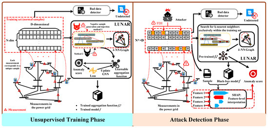
Figure 1.
SHAP-LUNAR-Based FDIA Detection Method.
3.1. Core Principles of LUNAR
LUNAR unifies local anomaly detection within the message-passing framework of GNNs. In this framework, each data sample is treated as a graph node, with edges representing sample similarity. Through message passing, LUNAR aggregates information from neighboring nodes to iteratively update target node representations. This process enables the model to learn complex feature representations, improving anomaly detection accuracy.
3.1.1. Unified Framework: Message Passing in GNNs
LUNAR integrates local anomaly detection methods into the GNN message-passing framework. Each data sample corresponds to a node, with edges defined by Euclidean distances between samples. Using message, aggregation, and update functions, LUNAR collects neighbor information and updates node representations.
The message function is defined as follows:
where represents the message from the source node j to the target node i, which is the edge feature corresponding to the distance ej,i between node samples.
We uniformly define the aggregation of messages from neighboring nodes as hNi(k);
The message-passing function φ determines the information content each neighbor node sends to the target node. The aggregation function T integrates multiple incoming messages into a single information stream through operations like average pooling or max pooling. In this study, the aggregation function is learnable rather than using traditional fixed operations like average pooling. Finally, the update function γ computes the subsequent hidden representation based on the aggregated information and the current node state. hi(0) = xi, where Ni denotes the set of adjacent nodes for node i, and hNi(k) represents the aggregated neighbor messages. hi(k−1) and hj(k−1) denote the representation vectors of the target node i and the neighbor node j in the (k − 1)-th layer, respectively. In summary, the k-th layer of the graph neural network (GNN) calculates node hidden representations through the aforementioned mechanism.
The update function is defined as follows:
This formula indicates that the aggregated message serves as the anomaly score for the target node.
3.1.2. Model Design: K-Nearest Neighbor Graph and Learnable Aggregation
Each data sample is represented as a node connected to its k-nearest neighbors, with edges weighted by Euclidean distances. Unlike fixed aggregation, LUNAR employs a neural network to learn optimal neighbor aggregation, enabling adaptability across datasets.
The k-nearest neighbor graph is constructed as follows:
For each sample xi, connect to its k-nearest neighbors j ∈ Ni, with edge features defined as follows:
The learnable aggregation function is defined as follows:
where F is a neural network with learnable parameters θ.
3.1.3. Negative Sample Generation: Enhancing Discriminative Capability
In unsupervised FDIA anomaly detection tasks, the training phase uses only normalized, attack-free normal samples. This avoids reliance on attack samples required by supervised data-driven methods, where attack samples are scarce and diverse, imposing high sample quality demands for supervised training. The proposed method introduces supervisory signals without incorporating attack samples by generating synthetic anomalies to simulate manual attacks. These anomalies must be distinguishable from normal samples but not overly simplistic, ensuring the model learns effective decision boundaries.
Anomaly generation methods include the following:
Uniform Distribution Method: Anomalies are sampled from a uniform distribution to cover data boundaries, formulated as follows:
where ε is a small positive constant.
Subspace Perturbation Method: Negative samples are generated by adding Gaussian noise to randomly selected feature dimensions of normal samples, formulated as follows:
where z~N(0, I), and M ∈ ℝd is a binary random vector in which each element is set to 1 with probability p and 0 otherwise, indicating the feature dimensions to be perturbed.
3.1.4. Loss Function and Training: Optimizing Anomaly Detection Performance
The model is trained to output anomaly scores of 0 for normal samples and 1 for attacked samples. Training is performed using the Adam optimizer, with model parameters selected based on validation set performance. The LUNAR loss function is defined as follows:
where yi is the label for sample xi (0: normal, 1: anomalous), and s(xi) is the model-predicted anomaly score.
In summary, the training workflow of the model is illustrated in Figure 2.
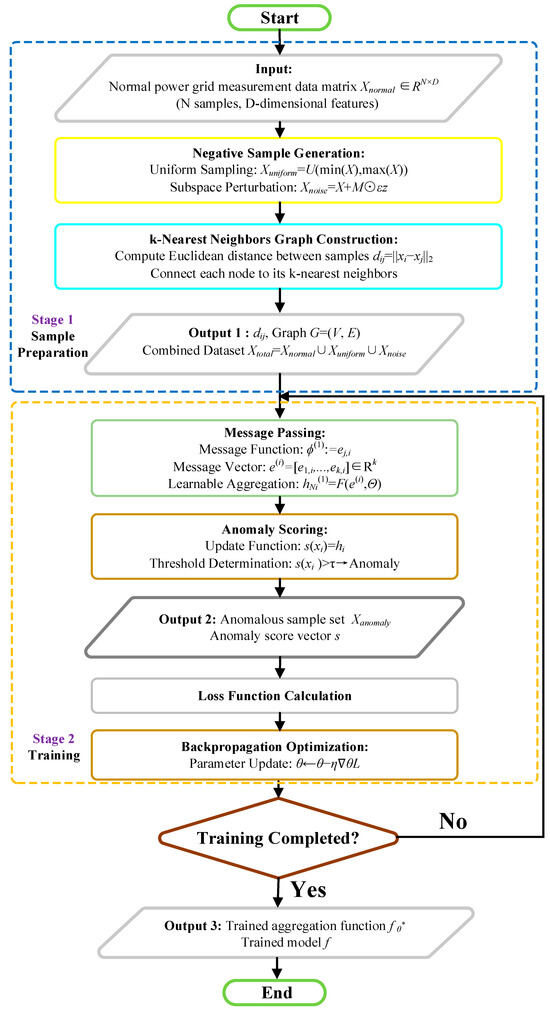
Figure 2.
LUNAR Training Workflow Diagram.
3.1.5. Robustness of LUNAR: Insensitivity to Neighbor Size
Traditional local anomaly detection methods are highly sensitive to the choice of k; varying k values can cause significant performance fluctuations. LUNAR employs a learnable aggregation function to extract effective information from all neighbor nodes, making it more robust to k selection. Experimental results demonstrate that LUNAR’s performance variance across different k values is substantially smaller than that of traditional methods.
3.2. SHAP-Driven Interpretability Enhancement for LUNAR
SHAP (SHapley Additive exPlanations) enhances machine learning model interpretability by quantifying feature contributions through Shapley values from cooperative game theory [26]. It provides explanations for individual predictions, clarifying how input features influence model decisions—specifically, the contribution of each sensor measurement to attack detection outcomes.
SHAP adapts the Shapley value concept from cooperative game theory to measure feature contributions. In this work, the Shapley value represents the average marginal contribution of a sensor measurement across all possible sensor measurement combinations, quantifying its impact on model predictions. For an attack detection model f and input features x, the SHAP value ϕi(x) denotes the contribution of feature i to the model’s predicted output, defined as follows:
where F is the full feature set, and S is a subset of F. The model prediction f(S) is computed over the feature subset S.
The main properties of SHAP are as follows:
- (1)
- Local interpretability: SHAP provides a local explanation for each prediction, where each predicted outcome can be decomposed into the sum of contributions from individual features plus a base value (representing the model’s prediction when no features are present).
- (2)
- Global interpretability: By aggregating SHAP values across all predictions, SHAP reveals the overall dependency and importance of features in the model.
- (3)
- Model-agnosticism: The SHAP method does not depend on the specific structure of the model and is applicable to any machine learning model, such as decision trees or neural networks.
In this study, we adopt KernelSHAP from SHAP as the approximation method. KernelSHAP is a model-agnostic approximation approach in the SHAP framework, whose core innovation transforms Shapley value computation into a weighted linear regression problem, as follows:
where, z′ is a binary vector indicating feature presence states (1 = present, 0 = absent). z represents the sample mapped from z′ to the original feature space. Specifically, for each feature, if z′i = 1, then zi = xi (original sample value); if z′i = 0, zi is replaced by a randomly selected value of that feature from the background dataset (typically the training set or random samples). πx(z′) denotes the Shapley kernel weights, defined as follows:
where |z′| indicates the number of active features.
Notably, unlike traditional SHAP methods such as TreeSHAP, KernelSHAP is fundamentally model-agnostic and can explain arbitrary black-box models. In contrast, TreeSHAP relies on tree model structures to achieve exact and efficient computation, making it applicable only to tree-based models.
In LUNAR-based FDIA detection for power grids, SHAP can explain model predictions. For instance, for anomalies detected as compromised, calculating SHAP values of their features identifies which features contribute most to the detection outcome. This helps researchers or engineers understand the model’s decision logic, trace attack pathways, and further optimize the model or implement targeted inspections and maintenance for the power grid.
It should be noted that while SHAP provides valuable feature-level interpretability by attributing anomaly scores to input sensor measurements, it cannot directly interpret the learned graph structures in the SHAP-LUNAR framework (i.e., k-nearest neighbor connections and learnable edge weights). In this framework, the graph structure is dynamically constructed based on inter-sample distances and further optimized through trainable aggregation functions. However, from a power grid application perspective, the graph structure itself maintains inherent interpretability: each node’s k nearest neighbors represent its most similar operational states in the feature space; analyzing the weighted contributions of neighbor nodes during aggregation helps understand local data manifold characteristics or reveal cluster structures of similar states (normal or attacked). Therefore, systematic exploration of interpretability for GNNs’ internal graph structures and aggregation mechanisms remains a promising direction for future research.
4. Case Study
4.1. Data and Parameter Settings
To evaluate the identification accuracy of the proposed algorithm on imbalanced samples under different scales, FDIA attacks with certain proportions were simulated in IEEE14 and IEEE118 systems. The FDIA mainly includes four typical attack types: (1) Pulse, (2) Random, (3) Ramping, and (4) Scaling. Notably, only samples affected by FDIA attacks by passing BDD were selected as attacked samples for testing. Measurement points were deployed at multiple buses or lines in power grids of different scales, where measurement values included bidirectional line power flows or bus power injections. We present the dataset information below in Table 1.

Table 1.
Sample Information.
As shown in Table 1, experiments employed IEEE 14-bus (19-dimensional PMU data) and IEEE 118-bus (180-dimensional PMU data) standard power systems, each containing 20,000 normal samples and 2000 FDIA samples. LUNAR parameters were systematically optimized as presented in Table 2.
Table 2.
Key LUNAR Parameters.
A learnable weighted aggregation mechanism (model_type = “WEIGHT”) was adopted, with neighbor number k = 130 covering the node degree distribution. Negative samples were generated through boundary uniform sampling (negative_sampling = “UNIFORM”) to simulate global anomalies. Contamination parameter (0.01) decoupled from real attack proportions prevents model overfitting. Min-Max scaling preserved physical constraints like voltage magnitude bounds ([0.95, 1.05] p.u.). This configuration balanced high-dimensional data processing requirements with power grid physical characteristics.
Notably, all experiments were validated on a Google Colab base configuration (single-core CPU @2.3 GHz, 12.7 GB RAM) without hardware acceleration.
4.2. Detection Accuracy Comparison Across Grid Scales
Four accuracy metrics were established in experiments: Accuracy (ACC), Precision (PRE), Recall (REC), and F1-score. FDIA detection results for IEEE14 and IEEE118 systems are recorded in Table 3 and Table 4.
Table 3.
FDIA Detection Results Under IEEE 14.
Table 4.
FDIA Detection Results Under IEEE 118.
In sensor systems of higher-dimensional complex power grids (IEEE 118-bus system), the graph-based method LUNAR demonstrates significant advantages with an F1-score of 96.79%. Its balanced precision (97.04%) and recall (96.55%) reflect deep adaptation to power grid samples. Through a learnable weight aggregation mechanism, this method dynamically focuses on latent connections between samples, maintaining high accuracy in 180-dimensional PMU data. In contrast, probabilistic unsupervised methods like GMM achieve 100% recall but suffer from over-sensitivity, as indicated by their low precision (89.73%). The Gaussian mixture model misidentifies normal fluctuations complying with Kirchhoff’s laws as attacks due to neglecting nonlinear constraints in power grids. Density estimation methods like COPOD completely fail in high-dimensional spaces (F1 < 25%), confirming the “curse of dimensionality” that undermines traditional probabilistic models.
Linear models (e.g., PCA and OCSVM) perform poorly on IEEE 118 (F1 ≤ 83.45%). Principal component analysis improves computational efficiency through dimensionality reduction but destroys latent sample features via linear projection, causing sharp increases in false alarms. Support vector machines fail to capture multi-pattern collaborative tampering in FDIA attacks due to linear kernels, resulting in a recall drop to 41.16%. These methods fundamentally compress physical mappings of power grids into linear spaces, creating decision boundaries that deviate from actual anomaly distributions.
The proximity-based representative LOF achieves an F1-score of 81.49% on IEEE 118, but its static aggregation rules pose risks. For example, detection accuracy may drastically change when neighbor count k varies, as fixed averaging cannot distinguish critical from minor sample connections. More critically, COF distorts density estimation in sparse regions through chain effects, yielding F1 scores below 20% and revealing inherent limitations of connectivity-based methods in circular power grid topologies. Outlier ensemble methods like FB improve F1 to 83.31% by integrating LOF/KNN, but remain significantly inferior to LUNAR, exposing their inability to deeply analyze feature differences between attacked and normal samples.
Neural network-based deep learning methods show polarization: AE/VAE achieves a maximum F1 of 94.61% on IEEE 14 through automated feature extraction, but becomes insensitive to localized attacks in IEEE 118 (F1 ≈ 83.45%). Adversarial generative models like ALAD completely fail against stealthy FDIA (F1 = 13.85%). The key limitation of these black-box models lies in decision-making opacity—operators cannot determine why specific nodes are flagged as anomalies. LUNAR, combined with SHAP interpretability analysis, could address this limitation in future work to assist attack path localization.
Supervised methods perform well in specific scenarios (e.g., random forests achieving F1 = 91.63 on IEEE 118) but face engineering deployment barriers due to dependency on attack labels. The “100% F1” of XGBOD on IEEE 14 is actually a dataset-specific coincidence. When tested on IEEE 118 data, XGBOD’s F1 score plummets to 43.88%. In contrast, LUNAR approaches supervised model accuracy through unsupervised learning by uniformly sampling negative samples to simulate unknown attack patterns, demonstrating unique value in label-scarce power grid environments. It achieves stable detection accuracy across different grid scales.
Cross-dimensional comparisons of two grid scales further validate core conclusions: In medium-scale grids (IEEE 14), LUNAR achieves near-perfect detection with 99.40% F1-score; in 180-dimensional complex grids (IEEE 118), it maintains 96.79% F1-score, representing a 2.21 percentage point improvement over the suboptimal unsupervised method GMM. This demonstrates LUNAR’s strong scalability and its ability to overcome the historical failure of traditional methods in high-dimensional dynamic systems.
4.3. Training and Detection Efficiency Comparison
To evaluate detection efficiency, we compare the proposed method with classical anomaly detection algorithms in terms of training and testing durations on both power grid datasets. Results are summarized in Table 5.
Table 5.
Training and Detection Efficiency of FDIA Methods.
From Table 5, we observe that LUNAR demonstrates industrial-level efficiency potential: the IEEE 118 test takes only 2.16 s, indicating its capacity to meet real-time PMU data processing requirements after further optimization. This efficiency stems from two key designs: (1) Input reduction from 180-dimensional raw PMU data to 130-dimensional distance vectors significantly lowers computational complexity; (2) Graph-structured parallelization enables node-independent computation. Comparative experiments show AE training consumes 207.78 s (12.7× LUNAR), making online updates impractical; LOF achieves faster training (10.57 s) but suffers a 13.03-s testing delay (6× LUNAR), failing real-time response. Lightweight COPOD (1.83-s test) achieves only 24.62% F1-score, revealing inherent accuracy-efficiency trade-offs. LUNAR approaches the accuracy-efficiency Pareto frontier with 16.35-s training and 2.16-s testing, providing reliable technical support for smart grid dynamic defense.
Theoretical complexity analysis further confirms LUNAR’s scalability. From the perspective of computational complexity for each component during training and testing: the k-NN graph construction scales as O(d n log n), while core message passing requires O(T n k d) for training and O(k d) per test instance (d: feature dimension, n: sample count, T: training epochs, k: neighbor count). SHAP interpreter (KernelSHAP) computational complexity is O(|S| M k d) (M: Monte Carlo sampling count, |S|: sample count requiring explanation). Despite high computational costs in the interpretation phase, constraining explanation sample count and implementing asynchronous execution strategies could achieve lower detection-plus-interpretation latency combinations in power systems.
The lightweight design enables deployment on SCADA edge computing nodes, which subscribe to PMU data streams via OPC UA interfaces. Notably, current testing did not employ hardware acceleration—deploying on substation edge devices equipped with NVIDIA T4 GPUs could further reduce latency. The integration proposal suggests containerized packaging interacting with the SCADA control layer through Modbus/TCP protocol, requiring minimal additional communication bandwidth to transmit anomaly localization results (SHAP feature contributions). This “edge detection + centralized alerting” hierarchical architecture avoids SCADA master station modification risks while satisfying IEC 62443-3-3 requirements for real-time threat response latency.
4.4. Comparison with Other Graph-Based Algorithms
To evaluate the advantages of the proposed method in FDIA identification accuracy and efficiency compared to other graph-based algorithms, we selected the classic unsupervised graph-based algorithm R-Graph for comparison. Results are summarized in Table 6.
Table 6.
Comparison Results Between the Proposed Method and R-Graph.
As shown in Table 6, R-Graph achieves over 90% accuracy on IEEE14 and 80% on IEEE118 tests. However, compared with the proposed algorithm, its accuracy is at least 5% lower in both cases. Additionally, its training and testing time is significantly higher, at least tenfold greater than the proposed method. This demonstrates the proposed algorithm’s substantial advantages in both precision and efficiency over R-Graph.
4.5. Parameter K Sensitivity Analysis
Algorithm sensitivity to hyperparameters critically impacts generalization capability. To investigate the proposed method’s sensitivity to key parameter k (number of neighbors), we test LUNAR against classical Proximity-Based methods on IEEE 118 under varying k values. Results are recorded in Table 7.
Table 7.
Detection Accuracy of Proximity-Based Methods at Different k Values.
Table 7 analysis reveals LUNAR’s strong robustness to neighbor count k as its distinguishing feature. In the IEEE 118 grid, when k increases from 5 to 150, LUNAR’s F1-score fluctuates only 0.21% (97.46%→97.25%), while KNN drops 15.76% (89.02%→73.26%). This advantage originates from neural network adaptability: learnable weights automatically filter redundant neighbors, preventing anomaly signal dilution. At k = 150, LUNAR assigns near-zero weights to low-correlation neighbors, focusing on critical topological connections. In contrast, KNN’s fixed averaging aggregates numerous irrelevant nodes at large k values, causing distorted anomaly detection. This feature reduces engineering maintenance costs: unlike conventional methods requiring frequent parameter tuning under dynamic grid topologies (e.g., line faults), LUNAR maintains performance across wide k ranges after single training. Except for KNN, all baseline methods exhibit significantly greater F1-score fluctuations across varying k values, with absolute performance inferior to LUNAR, failing to meet requirements for parameter robustness and detection accuracy.
4.6. Hyperparameter Sensitivity Analysis
Besides the core parameter k, sensitivity analysis of other parameters such as learning rate, epoch, and contamination is equally important. We present sensitivity analysis results under IEEE14 testing while keeping other parameters fixed. Table 8 lists the parameter values, and the results are recorded in Table 9.
Table 8.
Hyperparameter Value Settings.
Table 9.
Test Results Under Different Hyperparameters.
Table 9 presents parameter sensitivity analysis results (focusing on the IEEE 14 dataset), revealing key conclusions. Within the tested learning rate range (0.0001–0.01), the model demonstrates high stability. All learning rates achieve accuracy (ACC) above 0.9880 (98.80%) with most F1-scores approaching 1.0. For instance, at a 0.001 learning rate, ACC reaches 0.9988 and F1-score reaches 0.9935, indicating strong robustness against learning rate variations. Training epochs show minimal impact with slight performance fluctuations, suggesting good convergence. However, contamination rate emerges as a critically sensitive parameter. When the contamination rate increases to 0.1, the F1-score drops sharply to 0.9107 (9% decrease from near-optimal results) while precision (PRE) falls to 0.8361 (83.61%). This highlights the model’s weak adaptability to high contamination rates (increased anomaly proportions), requiring careful parameter calibration for reliable detection.
The proposed method demonstrates strong robustness against learning rate and epoch variations with minimal performance fluctuations, but elevated contamination rates significantly degrade detection capability, particularly affecting PRE and F1-score. This suggests that the contamination rate requires priority calibration in practical applications, while learning rate and epochs can vary within broad ranges. Parameter sensitivity differences validate the model’s stability under normal training conditions while revealing potential improvement directions for varying anomaly distributions.
4.7. K-Fold Cross-Validation Experiment
To verify the training and testing stability of the proposed method on the datasets, a k-fold cross-validation was conducted using ACC as the loss function. We set k = 5. The average loss and standard deviation (Std) results for training and testing are presented in Table 10.
Table 10.
K-Fold Cross Validation Summary.
As shown in Table 10, k-fold cross-validation results (k = 5) demonstrate the following: On the IEEE 14 dataset, the proposed method (Ours) achieves superior performance with a mean accuracy of 0.9943, significantly outperforming KNN (0.9088), LOF (0.9008), and COF (0.8823). It also attains the lowest standard deviation (0.0036), indicating optimal stability. On the IEEE 118 dataset, the proposed method maintains a leading mean accuracy (0.9809) with standard deviation (0.0043) only slightly higher than COF (0.0019). Notably, COF performs well on IEEE 118 (0.9778) but poorly on IEEE 14 (0.8823), revealing its sensitivity to data scale. Baseline models KNN and LOF show stable but lower accuracy across both datasets (0.90–0.91) with higher standard deviations (0.0037–0.0071), indicating limited generalization.
In summary, the proposed method achieves high accuracy and strong stability across datasets, particularly on IEEE 14. COF shows comparable performance on IEEE 118 but larger fluctuations in small-scale scenarios, while KNN and LOF demonstrate overall inferior performance. Cross-validation results confirm the proposed method’s superior robustness compared to mainstream models.
4.8. Statistical Significance Tests
Meanwhile, statistical significance tests play a critical role in validating the performance improvement of the proposed method. To statistically verify its effectiveness, paired t-tests were conducted against representative baseline models, with results summarized in Table 11 (dataset: IEEE 14; evaluation metric: F1-score).
Table 11.
Statistical Significance Test Results.
According to the statistical test results in Table 11, the following comprehensive analysis can be drawn: The proposed method demonstrates significant advantages over various baseline models in the FDIA detection task. The statistical significance of performance differences is confirmed by extremely high t-values (ranging from 100.7790 to 1390.4463) and highly significant p-values (all < 0.0001). Notably, Cohen’s d effect size metric ranges from 63.7383 to 879.3955, far exceeding Cohen’s threshold of 0.8 for large effect sizes, indicating substantial practical significance of performance differences. Specifically, the effect size of 63.7383 against GMM confirms the method’s substantial value, while the 879.3955 effect size against COF reveals fundamental limitations of traditional connectivity-based outlier factor algorithms in power grid anomaly detection. These results statistically validate the detection accuracy of the proposed method, where the learnable neighbor aggregation mechanism and graph neural network framework provide reliable technical solutions for smart grid security.
4.9. Ablation Studies
Ablation studies play a critical role in validating key components of the proposed method. To verify the importance of different sampling strategies in the sample generation module and the impact of using weighted distance summation for anomaly scoring, we conducted ablation experiments on the IEEE 14 and IEEE 118 datasets, as shown in Table 12. LUNAR I refers to generating a weight set for k distances with the anomaly score calculated as their weighted sum. LUNAR II directly outputs anomaly scores without weight generation. LUNAR I (without “SUBSPACE”) excludes subspace perturbation as negative sampling. LUNAR I (without “UNIFORM”) excludes uniform sampling. LUNAR I (Mixed) combines both negative sampling strategies.
Table 12.
Ablation Study Results on Sample Generation and Anomaly Scoring.
Based on the experimental results provided in Table 12, the following key conclusions can be drawn: First, the hybrid use of negative sampling strategies is critical. LUNAR I (Mixed) achieves optimal performance on both IEEE 14 and IEEE 118 datasets (ACC: 99.89%/99.41%, F1: 99.40%/98.21%). Removing subspace perturbation (without “SUBSPACE”) or uniform sampling (without “UNIFORM”) leads to performance degradation, particularly significant on IEEE 118 (F1 drops to 96.79% and 97.22%, respectively). This indicates complementary effects between the two negative sample generation methods—subspace perturbation simulates covert anomalies through local feature shifts, while uniform sampling covers explicit anomalies outside global distributions. Their combination provides more comprehensive guidance for learning decision boundaries. Secondly, the weighted distance aggregation mechanism is indispensable. LUNAR II (direct anomaly score output) shows severe performance deterioration, with F1 plummeting to 34.74% on IEEE 118. Compared with LUNAR I (outputting k distances’ weights and weighted summation), this proves that the learnable distance weighting mechanism constitutes the core advantage. It enables adaptive adjustment of neighbor importance rather than relying on fixed rules. This design significantly improves generalization capability on complex data. Additionally, IEEE 118 demonstrates higher sensitivity to design variations. Performance degradation across all ablation variants on IEEE 118 exceeds that on IEEE 14, with LUNAR II’s F1 collapsing to 34.74%, highlighting stringent requirements for anomaly scoring mechanisms in large-scale networks. Hybrid negative sampling achieves 1.4–1.5% F1 improvement over single strategies on this dataset, further confirming its necessity.
Ablation experiments confirm the synergistic value of subspace perturbation and uniform sampling, as well as the decisive role of weighted distance aggregation in model performance; their combination enables LUNAR to maintain high precision and robustness in complex scenarios.
4.10. Adversarial FDIA Sample Experiments
Investigating model performance under adversarial FDIA samples remains crucial. On IEEE 14, we employ a Wasserstein GAN with Gradient Penalty (WGAN-GP) generator to learn and generate adversarial samples that resemble normal data distributions yet evade detection. Attack samples with different perturbation magnitudes are generated, with 1000 samples per average perturbation magnitude. These are combined with normal samples from IEEE 14’s test set to evaluate the model’s detection capability against GAN-based covert FDIA attacks.
Based on test results of adversarial FDIA samples generated by Wasserstein GAN with Gradient Penalty (WGAN-GP) in Table 13, the proposed method demonstrates detection characteristics varying with perturbation intensity on the IEEE 14-bus system: At the minimum perturbation level (5.17%), the model achieves 92.93% accuracy, but the F1-score drops to 62.34% due to insufficient balance between precision (60.41%) and recall (64.40%), indicating that slightly perturbed adversarial samples can still effectively simulate the boundary of normal data distribution and partially evade detection mechanisms; When perturbation increases to 6.96%, recall significantly rises to 93.80%, reflecting enhanced sensitivity to moderate anomalies, with 74.44% precision producing an improved F1-score of 83.01%, revealing this perturbation range more easily triggers effective alarms; Under maximum perturbation (9.77%), recall reaches 99.20% peak but precision declines to 72.04%, suggesting excessive deviations from normal distribution are easily captured yet violate physical constraints, causing partial false alarms and resulting in 83.47% F1-score. This non-monotonic variation highlights the model’s dual sensitivity to perturbation magnitude-low perturbations challenge detection robustness through boundary ambiguity, while high perturbations enhance detectability through significant physical law violations, simultaneously implying future optimization potential for generative adversarial samples’ boundary adaptation capabilities against stealthier attack variants.
Table 13.
Adversarial FDIA Sample Experiment Results.
4.11. K-NN Graph Representation Evaluation
It should be noted that in the proposed method, graph nodes represent individual samples (i.e., measurement vectors at each time point), not physical nodes in the power grid. The graph structure reflects relationships between measurement samples rather than physical topology. To evaluate the k-NN graph’s representation capability for original data in the proposed method, we designed a k-NN graph evaluation experiment. PMU measurement data from IEEE 14-bus and IEEE 118-bus systems were used, analyzing 1000 time point samples each (including normal operation and FDIA attack samples). Parameter settings: k = 5 neighbors for the IEEE 14-bus system, k = 25 neighbors for the IEEE 118-bus system. Evaluation focuses on four core metrics: average degree reflecting graph connectivity density, clustering coefficient measuring local connection compactness, distance correlation evaluating graph-structure consistency with original data, and neighbor overlap testing local structure preservation capability. Evaluation results are shown in Table 14.
Table 14.
k-NN Graph Evaluation Results.
Experimental results reveal: in the IEEE14 system, the average degree is 5.48 ± 1.69, indicating actual connection counts slightly exceed the k value, reflecting sample interconnectivity; the IEEE118 system shows a higher average degree (33.42 ± 12.47), with its larger standard deviation (12.47) demonstrating increased sample connectivity variance in high-dimensional space. Both systems exhibit low average clustering coefficients (IEEE14: 0.1147; IEEE118: 0.1701), a characteristic suitable for anomaly detection since low clustering coefficients indicate samples lack tightly connected triangular relationships, facilitating differentiation between normal clusters and anomalies. Distance correlation metrics perform outstandingly, reaching 0.9459 (p < 10−15) for IEEE14 and maintaining 0.8587 (p < 10−12) for IEEE118, confirming k-NN graphs preserve global data structures effectively. Neighbor overlap ratios show IEEE14 achieves 67.17% while IEEE118 maintains 55.39%, indicating over half of the original neighbor relationships remain preserved in high-dimensional systems.
In-depth analysis reveals significant dimensionality effects. The IEEE118 system’s distance correlation declines by 0.0872 compared to IEEE14, with neighbor overlap ratio decreasing 12%, directly related to high-dimensional data sparsity. Calculated neighbor overlap decay rate (17.6%) aligns with the curse of dimensionality theory. Notably, despite high-dimensional representation degradation, k-NN graphs still provide solid foundations for the proposed method. Subsequent learnable graph aggregation mechanisms can further enhance representation capabilities. This design enables adaptive strengthening of critical connections and weakening of noisy edges, effectively compensating for high-dimensional structural loss.
Overall, experiments confirm k-NN graphs effectively represent sample relationships: global structure preservation (distance correlation > 0.85) and local neighborhood preservation (neighbor overlap > 55%) reach satisfactory levels. Though measurable representation degradation exists in high-dimensional systems, it remains within acceptable ranges. These findings provide theoretical foundations and design guidelines for optimizing GNN-based anomaly detectors on tabular data within high-dimensional dynamic systems.
4.12. SHAP-Based Interpretability Analysis
To enhance method interpretability, feature contribution heatmaps are generated for 20 attacked samples under IEEE 14 (19 total measurement variables). This is shown in Figure 3.
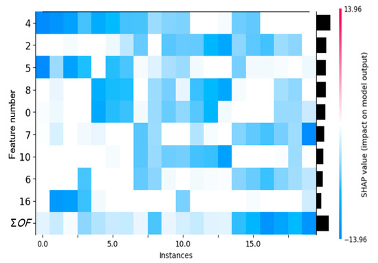
Figure 3.
SHAP Feature Contribution Heatmap (Note: ΣOF denotes Sum of 10 Other Features).
The heatmap’s x-axis represents power grid state samples across time points, with each sample corresponding to a PMU array data snapshot. The y-axis labels critical PMU sensor IDs (0, 2, 4…), which directly map to core monitoring nodes in the grid. Color mapping indicates SHAP value states: deep red marks high SHAP value ranges, while blue indicates low states. The right-side black bar length quantifies the absolute SHAP value sum, reflecting each sensor’s contribution magnitude to anomaly scores—negative values significantly elevate anomaly probability, whereas positive values suppress false alarms.
Sensor IDs carry explicit grid security implications: Sensor 4 dominates with the highest SHAP absolute value, whose anomaly fluctuations directly trigger FDIA detection; Sensor 2 contributes the second-highest SHAP absolute value, with pattern variations typically recognized by LUNAR as FDIA signatures; Sensor 5 ranks third in contribution among the 20 samples. Collectively, the nine explicitly displayed sensors show differential attention during detection, with contribution patterns varying across individual samples.
The heatmap reveals two attack patterns: In Sample 13, Sensors 2/8/10 synchronously display blue low-SHAP states, indicating attackers may manipulate correlated physical quantities collaboratively; In Sample 19, only Sensor 7 shows a blue peak, suggesting precise single-point tampering targeting critical sensors, which often evades traditional statistical detection. The bottom “Sum of 10 other features” bar quantifies residual sensor contributions—high values (e.g., Sample 16) imply distributed anomalies accumulating across multiple nodes, while near-zero values (e.g., Sample 2) confirm attack energy concentration on head sensors. This metric directly guides defense strategies: high residual contributions necessitate full-grid topology scanning, while low values prioritize critical equipment diagnostics.
The heatmap’s value lies in transforming LUNAR’s black-box decisions into actionable physical insights. A critical sensor’s high SHAP value pinpoints anomalies, aiding operators in tracing fault paths and attack vectors. Compared to traditional black-box models (e.g., VAE outputting only reconstruction errors), LUNAR achieves closed-loop defense from anomaly alerts to precise protection through sensor-level attribution—red hotspots not only mark attacked locations but also reveal tampering mechanisms, enabling both timely and targeted responses.
This visualization embodies spatial mapping of grid security logic: Dominant sensors (4/2/5) align with critical-node-first protection principles; multi-feature collaboration patterns expose attackers’ physical knowledge; the red-blue spectrum bridges abstract data to concrete device actions. When operators observe sustained blue alerts on key sensors, they recognize not just numerical anomalies but the causal chain of “cyberattacks inducing cascading failures”—a cognitive enhancement LUNAR brings to smart grid defense systems.
4.13. SHAP Explanation Fidelity Evaluation Experiment
To evaluate SHAP explanation fidelity, experiments were conducted using normal and attack samples from the IEEE14 dataset through feature perturbation strategies and Spearman rank correlation analysis. Experimental settings: For each sample, the top 5 SHAP-ranked features (r = 5) were selected, with 5 independent perturbation trials (trials = 5) per feature. Perturbation involved replacing target feature values with distribution-matched values from normal datasets, calculating absolute anomaly score changes caused by feature perturbations. The fidelity metric was defined as the Spearman correlation coefficient (ρ) between SHAP feature importance ranking and measured impact ranking, with a value range [−1, 1]. ρ > 0.8 indicates a strong correlation. Evaluation results are shown in Table 15.
Table 15.
SHAP Explanation Fidelity Evaluation Results.
The experimental results show that the fidelity of attack samples reaches 1.0 ± 0.0, indicating SHAP’s feature importance ranking on attack samples perfectly matches the model’s actual sensitivity ranking to feature perturbations (i.e., when SHAP-identified important features are replaced with normal values, the maximum output change occurs). The fidelity of normal samples is lower (0.4), suggesting SHAP’s feature importance ranking shows weaker consistency with the model’s actual behavior on normal samples. This may result from inherently low anomaly scores in normal samples, where feature perturbations cause minimal score changes, increasing ranking randomness. The overall sample fidelity (0.7) falls between these values, primarily driven by the high fidelity of attack samples. This confirms SHAP explanations are reliable for attack samples but less interpretable for normal samples, aligning with practical needs where attack sample explanations are prioritized. These results validate SHAP’s high reliability in attack diagnosis scenarios, despite weaker consistency under normal conditions. However, since smart grid security applications mainly focus on attack analysis, this characteristic meets engineering requirements.
4.14. SHAP Computation Parameter Sensitivity Analysis
The background dataset size parameter affects SHAP explanation efficiency. To evaluate this impact on the IEEE 14-bus system, this study conducted sensitivity experiments on the background dataset sampling parameter n during SHAP interpreter initialization. Experiments focused on assessing how varying n (the number of synthesized samples approximating background expectations) affects single-sample explanation efficiency. As shown in Table 15, parameter n was systematically set to 10, 50, and 100, and the average computation duration for generating SHAP explanations per sample was precisely measured. Results are recorded in Table 16.
Table 16.
Experimental Results of SHAP Explanation Fidelity Evaluation.
The results clearly show that parameter n significantly and approximately linearly increases the explanation computation duration. When n = 10, the average per-sample explanation duration was 2.1797 s; increasing n to 50 raised the computation time to 10.6124 s; further increasing n to 100 caused a sharp rise in computational burden, with average duration reaching 21.1023 s. This directly confirms that increasing background sample size n, while potentially improving Shapley value estimation reliability, inevitably causes significant increases in explanation computation costs. The computation duration growth trend with n provides critical empirical evidence for selecting appropriate n values in practical applications to balance explanation accuracy requirements and computational efficiency.
5. Conclusions
This paper addresses the challenges in detecting false data injection attacks (FDIA) in smart grids, including high parameter sensitivity, inefficient high-dimensional data processing, strong dependency on labeled data, and lack of interpretability. We propose an unsupervised detection framework based on SHAP-LUNAR, achieving breakthroughs through the following three contributions:
- (1)
- Learnable graph-based anomaly detection architecture: A lightweight k-nearest neighbor graph is constructed. By leveraging the message passing mechanism of graph neural networks (GNN), this method unifies local anomaly detection approaches and incorporates learnable aggregation functions to dynamically integrate neighbor information. Experiments demonstrate significantly reduced sensitivity to the key parameter k: when k increases from 5 to 150 in the IEEE 118 system, the F1-score fluctuation is only 0.21%, compared to 15.76% for traditional methods like KNN.
- (2)
- Unsupervised training mechanism: Boundary-uniform sampling generates negative samples to simulate attack patterns, eliminating reliance on scarce attack labels. The method achieves F1-scores of 99.40% and 96.79% on IEEE 14/118 systems, respectively, improving by 6.54% and 2.21% over the best unsupervised baseline (GMM). For high-dimensional scenarios (180 dimensions in IEEE 118), detection time is only 2.16 s, 6 times faster than LOF.
- (3)
- Enhanced interpretability: SHAP values quantify each sensor feature’s contribution to anomaly scores. Generated heatmaps accurately localize critical attack features (e.g., meter measurements 4/2/5 with the highest contribution) and distinguish coordinated tampering from single-point attacks, providing actionable defense insights for operators.
Limitations include: (1) Negative sample generation relies on uniform distribution assumptions, potentially missing complex attack patterns; (2) Current experiments use static topologies without considering grid dynamic reconfiguration. Future work will explore advanced sample generation strategies for sophisticated attacks and adaptive solutions for dynamic topologies, incorporating physical constraints to enhance sample rationality. Additionally, future work may incorporate time-varying graphs or topology-invariant GNN models, and connect with practical scenarios like renewable energy integration and self-healing grids. (3) This paper focuses on addressing the overall interpretability of black-box models and discusses feature-level interpretability, but does not fully resolve the interpretability of the GNN itself and its internal graph structure. Future work will further explore interpretability methods for GNN internal graph structures and aggregation mechanisms.
In conclusion, the proposed method provides a reference solution for FDIA detection in smart grids with high accuracy, strong robustness, high efficiency, and interpretability. Its integrated “unsupervised training-graph structure learning-attribution explanation” architecture offers universal value for anomaly detection in high-dimensional dynamic systems.
Author Contributions
Conceptualization, J.L. and H.G.; methodology, J.L.; software, H.G.; validation, H.K., X.H. and S.L.; data curation, D.Z., G.L. and Z.R.; writing—original draft preparation, J.L. and H.G.; writing—reviewing and editing, J.L. and H.G.; visualization, Y.L. and W.Z.; supervision, K.-W.L.; project administration, K.-W.L.; funding acquisition, J.L. All authors have read and agreed to the published version of the manuscript.
Funding
This research was funded by the Science and Technology Project of China Southern Power Grid Company Limited (Project Name: Security Protection Technologies against Data Anomalies and Cyber Attacks in Urban Integrated Energy Cyber-Physical System, Project Number: 031900KC23120066).
Data Availability Statement
The data presented in this study are available on request from the corresponding author. The data are not publicly available due to institutional restrictions.
Conflicts of Interest
Author Jinman Luo, Huichao Kong, Shimei Li, Guozhang Li, Yuan Li and Weile Zhang were employed by the company Dongguan Power Supply Bureau of Guangdong Power Grid Corporation. The authors declare that this study received funding from China Southern Power Grid Company Limited. The funder was not involved in the study design, collection, analysis, interpretation of data, the writing of this article or the decision to submit it for publication.
References
- Li, H.; Li, T.; Chen, T.; Zhao, G. A Detection Based on OMES and MTAD-GAT for False Data Injection Attack in Smart Grid. In Proceedings of the 2022 IEEE 6th Conference on Energy Internet and Energy System Integration (EI2), Chengdu, China, 11–13 November 2022; pp. 1578–1584. [Google Scholar]
- Li, N.; Zhang, J.; Ma, D.; Ding, J. Enhancing Detection of False Data Injection Attacks in Smart Grid Using Spectral Graph Neural Network. IEEE Trans. Ind. Inform. 2025, 21, 4543–4553. [Google Scholar] [CrossRef]
- Li, X.; Wang, Y.; Lu, Z. Graph-based detection for false data injection attacks in power grid. Energy 2023, 263, 125865. [Google Scholar] [CrossRef]
- Wu, S.; Yang, C.; Wang, J.; Shi, D. A Lightweight Framework for Measurement Causality Extraction and FDIA Localization. IEEE Trans. Smart Grid 2025, 16, 2587–2598. [Google Scholar] [CrossRef]
- He, Y.; Huang, Z.; Vogt, S.; Sick, B. PrOuD: Probabilistic Outlier Detection Solution for Time-Series Analysis of Real-World Photovoltaic Inverters. Energies 2023, 17, 64. [Google Scholar] [CrossRef]
- Wei, S.; Wu, Z.; Xu, J.; Hu, Q. Multiarea probabilistic forecasting-aided interval state estimation for FDIA identification in power distribution networks. IEEE Trans. Ind. Inform. 2023, 20, 4271–4282. [Google Scholar] [CrossRef]
- Hu, D.; Dong, Y.; Wang, J.; Shi, D. Detection of false data injection attacks in smart grids under power fluctuation uncertainty based on deep learning. In Proceedings of the International Conference on Power System Technology (PowerCon), Jinan, China, 21–22 September 2023; pp. 1–6. [Google Scholar]
- Patel, V.; Kapoor, A.; Sharma, A.; Chakrabarti, S. Taxonomy of outlier detection methods for power system measurements. Energy Convers. Econ. 2023, 4, 73–88. [Google Scholar] [CrossRef]
- Qu, Z.; Yang, J.; Wang, Y.; Georgievitch, P.M. Detection of false data injection attack in power system based on Hellinger distance. IEEE Trans. Industr. Inform. 2023, 20, 2119–2128. [Google Scholar] [CrossRef]
- Zu, T.; Li, F. Self-Attention Spatio-Temporal Deep Collaborative Network for Robust FDIA Detection in Smart Grids. Comput. Model. Eng. Sci. 2024, 141, 1395–1417. [Google Scholar] [CrossRef]
- Komadina, A.; Martinić, M.; Groš, S.; Mihajlović, Ž. Comparing threshold selection methods for network anomaly detection. IEEE Access 2024, 12, 124943–124973. [Google Scholar] [CrossRef]
- Yang, X.; Wang, Z.; Zi, X. Thresholding-based outlier detection for high-dimensional data. J. Stat. Comput. Simul. 2018, 88, 2170–2184. [Google Scholar] [CrossRef]
- Yu, K.; Chen, H. Markov boundary-based outlier mining. IEEE Trans. Neural Netw. Learn. Syst. 2019, 30, 1259–1264. [Google Scholar] [CrossRef]
- Mukhriya, A.; Kumar, R. Combination fairness with scores in outlier detection ensembles. Inf. Sci. 2023, 645, 119337. [Google Scholar] [CrossRef]
- Liu, F.T.; Kai, M.T.; Zhou, Z.-H. Isolation-based anomaly detection. ACM Trans. Knowl. Discov. Data 2012, 6, 1–39. [Google Scholar] [CrossRef]
- Thomas, R.; Judith, J.E. Voting-based ensemble of unsupervised outlier detectors. In Advances in Communication Systems and Networks: Select Proceedings of ComNet 2019; Springer: Singapore, 2020; pp. 501–511. [Google Scholar]
- Bii, J.K.; Rimiru, R.; Mwangi, R.W. Adaptive boosting in ensembles for outlier detection: Base learner selection and fusion via local domain competence. ETRI J. 2020, 42, 886–898. [Google Scholar] [CrossRef]
- Ida Evangeline, S.; Darwin, S.; Peter Anandkumar, P.; Chithambara Thanu, M. Anomaly detection in smart grid using a trace-based graph deep learning model. Electr. Eng. 2024, 106, 5851–5867. [Google Scholar] [CrossRef]
- Ding, Y.; Ma, K.; Pu, T.; Wang, X.; Li, R.; Zhang, D. A deep learning-based classification scheme for cyber-attack detection in power system. IET Energy Syst. Integr. 2021, 3, 274–284. [Google Scholar] [CrossRef]
- Reda, H.T.; Anwar, A.; Mahmood, A.N.; Tari, Z. A taxonomy of cyber defence strategies against false data attacks in smart grids. ACM Comput. Surv. 2023, 55, 1–37. [Google Scholar] [CrossRef]
- Pinto, S.J.; Siano, P.; Parente, M. Review of cybersecurity analysis in smart distribution systems and future directions for using unsupervised learning methods for cyber detection. Energies 2023, 16, 1651. [Google Scholar] [CrossRef]
- Li, R.; Chen, H.; Liu, S.; Li, X.; Li, Y.; Wang, B. Incomplete mixed data-driven outlier detection based on local–global neighborhood information. Inf. Sci. 2023, 633, 204–225. [Google Scholar] [CrossRef]
- Sun, L.; Zhou, K.; Zhang, X.; Yang, S. Outlier data treatment methods toward smart grid applications. IEEE Access 2018, 6, 39849–39859. [Google Scholar] [CrossRef]
- Li, H.; Dou, C.; Yue, D.; Hancke, G.P.; Zeng, Z.; Guo, W.; Xu, L. End-edge-cloud collaboration-based false data injection attack detection in distribution networks. IEEE Trans. Industr. Inform. 2023, 20, 1786–1797. [Google Scholar] [CrossRef]
- Goodge, A.; Hooi, B.; Ng, S.K.; Ng, W.S. Lunar: Unifying local outlier detection methods via graph neural networks. Proc. Conf. AAAI Artif. Intell. 2022, 36, 6737–6745. [Google Scholar] [CrossRef]
- Lundberg, S.M.; Lee, S.-I. A Unified Approach to Interpreting Model Predictions. arXiv 2017, arXiv:1705.07874. [Google Scholar] [CrossRef]
Disclaimer/Publisher’s Note: The statements, opinions and data contained in all publications are solely those of the individual author(s) and contributor(s) and not of MDPI and/or the editor(s). MDPI and/or the editor(s) disclaim responsibility for any injury to people or property resulting from any ideas, methods, instructions or products referred to in the content. |
© 2025 by the authors. Licensee MDPI, Basel, Switzerland. This article is an open access article distributed under the terms and conditions of the Creative Commons Attribution (CC BY) license (https://creativecommons.org/licenses/by/4.0/).