Article

Optimization Design of Microwave Filters Based on Deep Learning and Metaheuristic Algorithms

College of Transportation, Inner Mongolia University, Hohhot 010021, China
*
Author to whom correspondence should be addressed.
Electronics 2025, 14(16), 3305; https://doi.org/10.3390/electronics14163305
Submission received: 8 July 2025 / Revised: 4 August 2025 / Accepted: 18 August 2025 / Published: 20 August 2025

Abstract

To address the efficiency bottlenecks of traditional full-wave simulation methods in the high-performance design and rapid optimization of microwave filters, this study proposes an efficient design method based on an improved surrogate model and a hybrid optimization algorithm. A one-dimensional dense convolutional autoencoder (1D-DenseCAE) model is constructed to enhance the model’s ability to extract key features and improve convergence speed. Additionally, the Ivy–Hiking optimization algorithm (IHOA) is introduced, combining the advantages of global search and local fine-tuning. Experiments demonstrate that this method achieves approximately a 25% improvement in convergence speed over the standard one-dimensional convolutional autoencoder (1D-CAE) in cavity filter design, and enables efficient optimization in complex structures such as interdigital filters and seventh-order cross-coupled cavity filters, meeting design requirements of return loss below −20 dB and in-band ripple under 0.5 dB. This method provides an effective technical pathway for the intelligent design of microwave filters.

1. Introduction

Microwave filters represent a pivotal component within contemporary wireless communication systems, exerting a direct influence on the systems’ signal selectivity and their capacity to withstand interference. Electromagnetic (EM)-based yield optimization is a challenging task in microwave design due to its need for extensive EM simulations, which are typically time-consuming [1]. Employing EM-based fine models within the traditional Monte Carlo (MC) framework incurs prohibitive computational costs, owing to the extensive EM simulations required to achieve significant yield improvement [2]. Developing efficient yield-driven optimization techniques for microwave systems with high computational costs has been the objective of substantial research efforts throughout the last decade [3,4,5,6,7].
Significant progress has been made in the research and application of surrogate models in the field of microwave. In 2020, Zhang et al. proposed a neuro-TF-based surrogate model [1]. In terms of optimization methods in the microwave field, Jin et al. proposed an advanced cognition-driven electromagnetic optimization approach based on a transfer-function feature-based surrogate model [8]. Zhao et al. put forward a homotopy optimization approach using an artificial neural network (ANN)-based surrogate model [9]. Compared with conventional ones, these methods considerably improve computational efficiency. Subsequently, a hybrid surrogate model-assisted evolutionary algorithm for filter optimization (H-SMEAFO) method [10], an AI-assisted surrogate modeling and optimization (SAO) method [11], a pattern search optimization-based surrogate modeling space definition (PSOMSD) method [12], and an offline surrogate model-assisted evolutionary algorithm [13] were proposed. These have effectively cut electromagnetic simulation costs and shortened the design cycle.
In recent years, studies in this field have introduced methods like neural networks and spatial mapping into surrogate models. For example, a microwave microfluidic sensor optimization and design approach based on the particle-ant colony optimization algorithm (PACO) and wolf colony algorithm (WCA) has been proposed [14]. By optimizing the microfluidic channel routing, the sensor sensitivity was enhanced by approximately 78.6%. An improved biogeography-based optimization algorithm with multiple adaptive mutation operators (BBOIMAM) [15] was proposed to strengthen local search abilities. Recent innovations have integrated response feature extraction technology with the particle swarm optimization (PSO) algorithm [16], resulting in a significant reduction in the required number of training data points. The Ivy algorithm (IVYA) [17] exhibits remarkable global exploration and diversity maintenance capabilities, offering extensive solution-space coverage during optimization. However, it is relatively less effective in fine-tuning near solutions. The Hiking optimization algorithm (HOA) [18] excels at leveraging “gradient” information for local solution fine-tuning, achieving high-precision convergence. However, when used alone, it may encounter premature convergence or insufficient global exploration in complex, high-dimensional problems. In order to address the aforementioned challenges, a hybrid approach combining IVYA and HOA can be adopted. In the early search phase, the IVYA mechanism is dominant, utilizing the diffusion growth strategy of ivy to extensively explore the solution space and rapidly identify several regions in close proximity to the global optimum. In the subsequent search phase, the local search mechanism of HOA is introduced. The utilization of gradient information, in conjunction with the direction provided by a lead hiker, serves to further explore the regions of potential solution identified in the initial stages of the process. This approach enables the refinement of filter parameters, thereby ensuring the optimal performance of the system. The present paper puts forward a collaborative innovation framework based on a “surrogate model optimization algorithm”:
  • The proposed 1D-DenseCAE surrogate model incorporates cross-layer feature reuse through DenseNet [19] (densely connected convolutional network) connectivity, effectively mitigating the gradient-vanishing problem. Furthermore, the embedded efficient channel attention (ECA-Net) mechanism dynamically weights key frequency-band features, enhancing the accuracy of S-parameter prediction.
  • The IHOA integrates IVYA’s population-collaborative diffusion mechanism with HOA’s terrain-adaptive step-length strategy, establishing a closed-loop optimization framework that balances global exploration and local exploitation.
  • The 1D-DenseCAE surrogate model substitutes electromagnetic simulation for fitness evaluation in the optimization process. When integrated with IHOA, this combined approach enables efficient exploration of the parameter space.
Experimental results demonstrate 25% faster convergence with the 1D-DenseCAE model compared to conventional 1D-CAE for cavity filter optimization. Notably, the IHOA integrated with 1D-DenseCAE achieves significant performance in diverse complex microwave filters, satisfying stringent specifications, including passband return loss below −20 dB and in-band ripple under 0.5 dB. This work provides a robust theoretical foundation and an efficient computational framework for high-performance microwave filter optimization.

2. Construction of the 1D-DenseCAE Surrogate Model

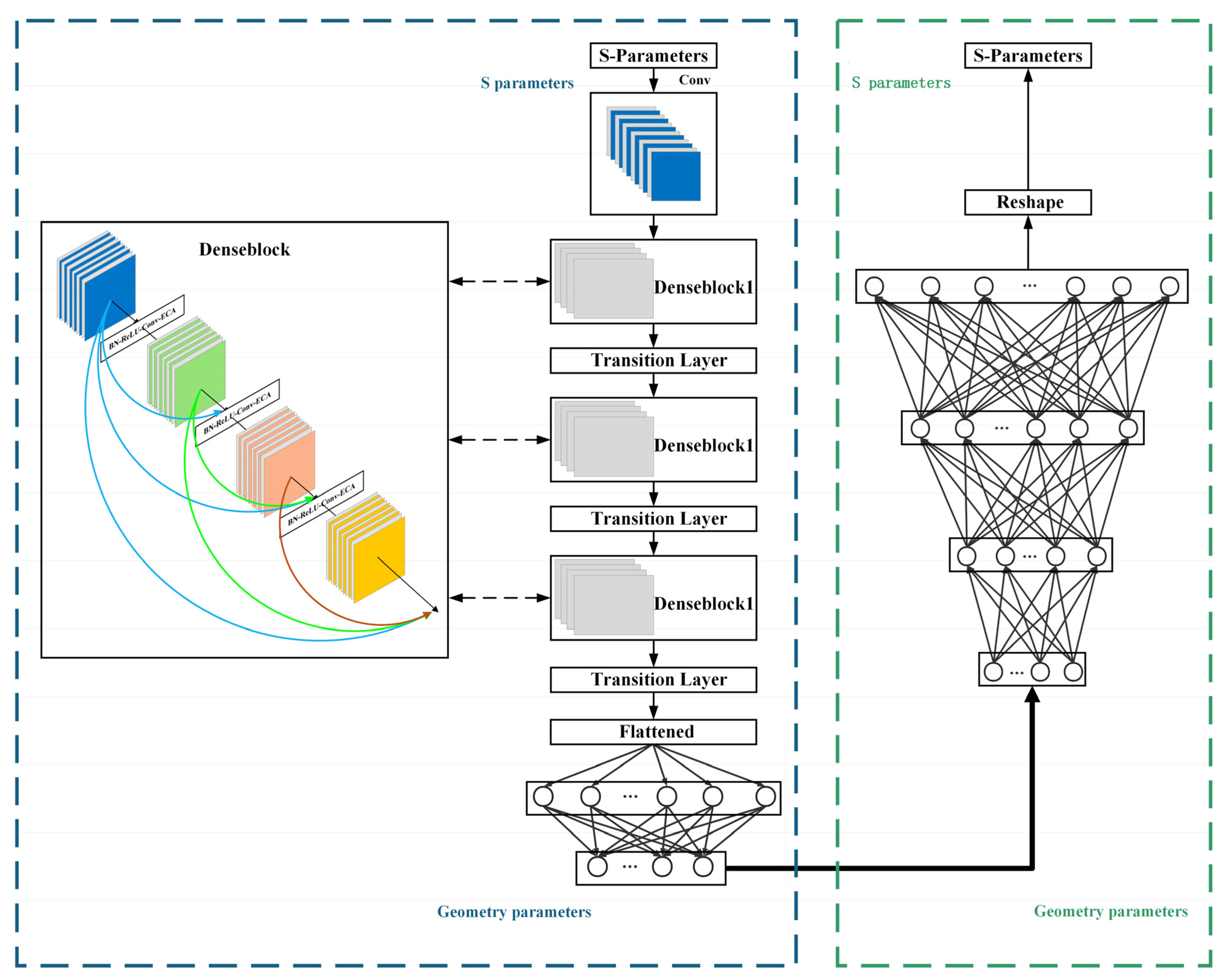
Manufacturing errors can significantly degrade filter performance. Thus, obtaining a filter design robust to such errors is crucial. However, the main challenge in filter yield optimization is efficiency. To address this, surrogate models have been proposed [20,21,22,23]. Surrogate models are computationally cheap approximation models mapping the filter design parameters to the filter responses or features extracted from filter responses [1]. As the most advanced technique for feature learning with convolution kernels in an unsupervised way, the convolutional autoencoder (CAE) has been recently developed to tackle the issue of feature extraction for classification tasks [24]. However, standard CAE has limitations: it depends heavily on random initialization and data statistics and lacks explicit control over the physical significance of filters, shape adaptability, feature diversity, and sensitivity to subtle features. There is also a risk that optimization goals may not fully align with final application objectives. To address these issues, we improve upon the standard CAE and introduce the 1D-DenseCAE surrogate model. The network structure comprises two core components: an encoder and a decoder. The encoder transforms input S-parameter responses (including real and imaginary parts) into corresponding geometric design parameters. The decoder performs the reverse mapping, reconstructing the S-parameters from geometric parameters. The key innovation lies in integrating a dense feature reuse mechanism and channel attention guidance, significantly enhancing prediction accuracy and generalization ability. The model architecture is illustrated in Figure 1.

2.1. Encoder: Multi-Scale Feature Extraction

The encoder compresses the input S-parameters (dimension [400, 2]) into a 256-dimensional latent vector through hierarchical feature extraction. The first layer is a 1D convolutional layer with 16 filters of size 3 and stride 1, producing a feature map of [400, 16]. Three cascaded DenseBlocks perform deep abstraction; each contains four convolutional layers (with 3 × 3 kernels), utilizing dense connections to maximize feature reuse and gradient propagation. An efficient channel attention (ECA) module (with a 1D convolutional kernel of size 3) follows each convolutional layer, adaptively weighting key channels. Transition layers, incorporating downsampling with stride 2, connect the blocks and progressively compress the spatial dimensions ([400, 64] → [200, 32] → [100, 44] → [50, 44]), while expanding the receptive field. Finally, the feature maps are flattened and passed through a fully connected layer to generate the latent representation.

2.2. Decoder: High-Fidelity Response Reconstruction

The decoder maps the 256-dimensional latent vector back to the original S-parameter space of [400, 2]. The first fully connected layer (256 nodes, Mish activation [25]) decodes the latent features. The second fully connected layer (1024 nodes, Mish activation) expands the feature dimensionality. The third fully connected layer (800 nodes, Mish activation) outputs a vector reshaped into a [400, 2] matrix, reconstructing the S-parameter response.

2.3. Loss Function

During the training of the 1D-DenseCAE model, the loss function is based on reconstruction error, aiming to evaluate the model’s ability to reconstruct the input data. The mathematical expression is as follows:
L rec = 1 N i = 1 N | T real , i T pred , i |
In this context, T real , i denotes the actual value input to the encoder, and T pred , i represents the reconstructed value output by the decoder.
The specific technical details of the constructed 1D-DenseCAE model are depicted in Figure 2. Table 1 presents a comprehensive overview of the main parameter configurations for the 1D-DenseCAE model, including layer names, the scale of nodes or convolutional kernels, stride, output shape, and the activation functions utilized.

3. Design of IHOA

To address local optima entrapment and slow convergence in microwave filter optimization, this study proposes the IHOA. The IHOA implementation process is as follows. During initialization, the population is generated using max–min Latin hypercube sampling (LHS) [26] to ensure uniform coverage of the solution space. In the global search phase, the IVYA is employed to simulate vine spreading behavior [18]. Individuals sense the direction of the global optimum and dynamically adjust their positions for extensive exploration. For local optimization, the best-performing individuals are selected, and the HOA is applied. Utilizing Tobler’s hiking function [27] to dynamically adjust step sizes, position updates incorporate global guidance and random perturbations. Boundary handling ensures solution validity. Throughout iterations, global spreading and local exploitation alternate. Elite individuals are retained until the maximum iterations or a convergence threshold is met, and the global optimum is ultimately output.

3.1. Mathematical Models of Algorithm Components

3.1.1. Mathematical Model of the IVYA Global Search Module

The IVYA module drives population diffusion via a vine-growth-based model, exploring the global optimum through fitness guidance and position updates. Its formula for calculating the global optimum X best is as follows:
X best = arg min X i Pop f X i
Here, f X i represents the fitness of individual X i , and Pop denotes the current population. The position update mechanism enables individuals to adjust their growth direction according to the global optimum. The update formula is as follows:
X i new = X i + α X best X i
Here, X i is the current position of individual i , and α is the factor controlling the guidance strength of individuals towards the global optimum.
The module mimics vine phototropism [28]. Within the maximum iterations, it updates individuals’ growth rates and positions, calculates new fitness values, and decides on accepting new positions. After each iteration, it updates the global optimal individual and fitness, finally outputting the global optimum. Through population collaboration and adaptive search, IVYA efficiently optimizes in complex spaces.

3.1.2. The HOA Local Optimization Module

The HOA module performs a sophisticated search on the premium solution regions that have been generated by the IVYA module. The system performs exhaustive local solution mining through velocity modelling and position updates. The velocity modeling adopts the Tobler hiking function:
V i , t = 6 exp 3.5 tan θ i , t + 0.05
Here, V i , t is the velocity of individual i at iteration t , and θ i , t 0 ,   50 is the random slope angle used to simulate the steepness of terrain. After obtaining the walking velocity, each individual performs a guided-offset update based on the position information of the current global best individual X best . The position update formula is as follows:
X i , t + 1 = X i , t + V i , t + γ i , t X best α i , t X i , t
In the above formula, X i , t is the current position of individual i ; α i , t is the sweeping factor, controlling the offset intensity of individuals from the optimal direction, with α i , t [ 1,2 ] ; γ i , t is the perturbation coefficient, indicating the adjustment amplitude of the individual update direction, and γ i , t 0,1 . By dynamically adjusting velocity and position, HOA conducts a fine-grained local search to avoid falling into a local optimum.

3.2. A Case Study of Filter Design Based on Surrogate Model and IHOA

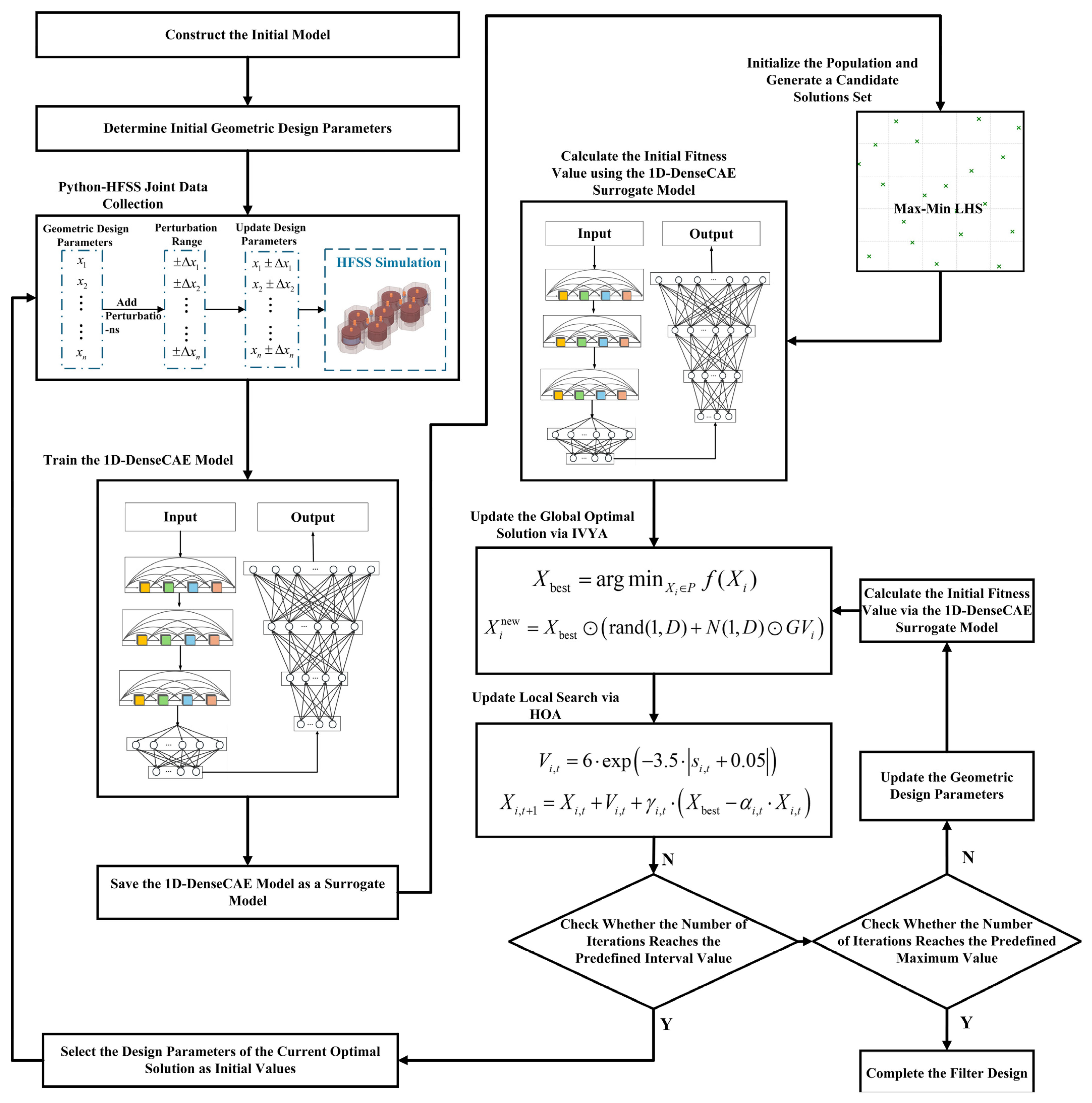
Figure 3 illustrates the design process driven by the 1D-DenseCAE model and IHOA. The 1D-DenseCAE surrogate model, trained on EM simulation data by integrating DenseNet and ECA-Net, accurately captures the mapping between filter geometry and S-parameters. The trained model is integrated into the IHOA framework, which combines IVYA and HOA. These algorithms work together to iteratively optimize filter design parameters until preset performance criteria are met, significantly boosting design efficiency without sacrificing accuracy.
IHOA first initializes the population and related parameters and then enters the main loop. After performing a global and local search, the algorithm screens the population based on the fitness results and dynamically adjusts the step size to improve convergence and search accuracy. Finally, when the termination conditions are met, the global optimal solution and its corresponding filter performance are output. The algorithm implementation process is detailed in Algorithm 1.
Algorithm 1: IHOA (data processing automation and output reading)
Input: Population size N p o p , dimension D, search bounds   I m a x and I m i n , max iterations MaxIter
Output: Global best individual   I b e s t and its fitness   f b e s t
1. Initialize the population using LHS
2. Evaluate the fitness of all individuals
3. Identify current global best   I b e s t and   f b e s t
4. For each iteration until the maximum iteration limit is reached:  // IVYA’s global search
5. Generate a new candidate solution by updating position based on global diffusion (Use the IVYA strategy to simulate growth and expansion)
6. If the new fitness is better, Then update the current individual with this new solution
7. Rank individuals based on fitness and select the top-K with the highest fitness for local refinement
8. For each of the selected K individuals:  // HOA’s local optimization
9. Randomly generate a terrain slope angle between 0° and 50°
10. Compute walking velocity based on slope using Tobler’s hiking function
11. Calculate a global guidance component to follow the current global best
12. Update the individual’s position based on walking direction and velocity
13. If the new solution improves fitness, Then replace the original individual
14. Return the best solution ( I b e s t ) and its corresponding fitness ( f b e s t )

4. Experimental Results and Discussion

4.1. Validation of the 1D-DenseCAE Model

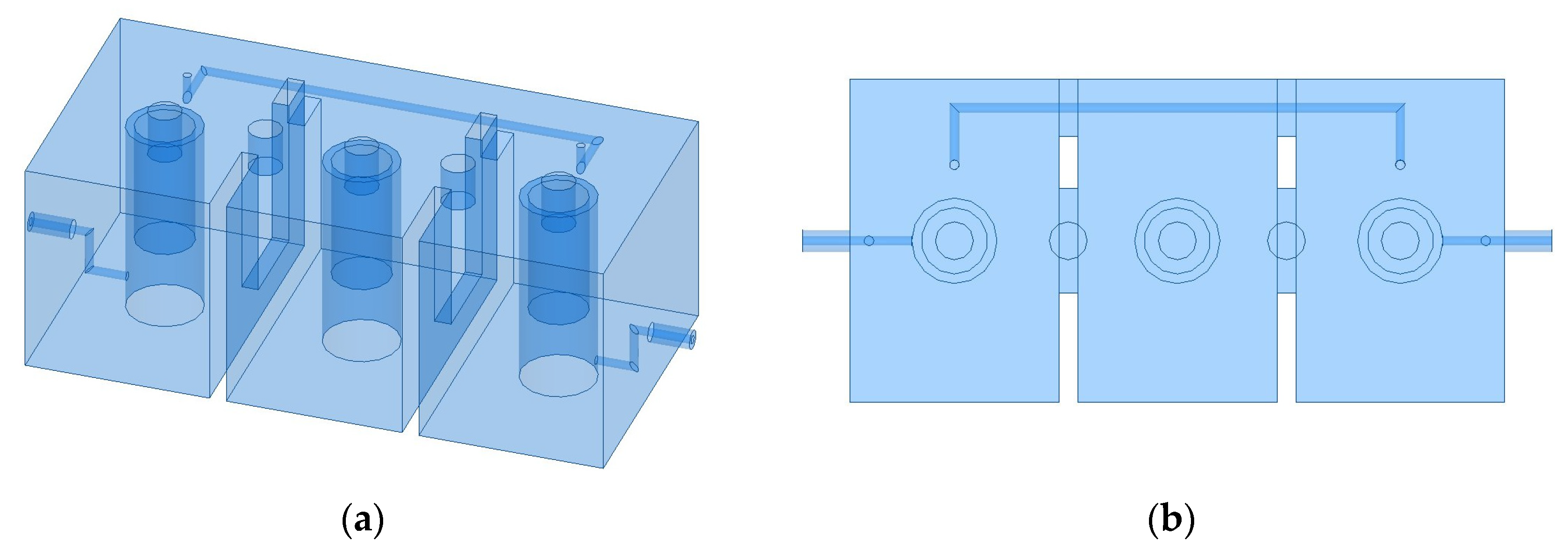
This section validates the 1D-DenseCAE model using a cavity filter model (Figure 4). Data were collected via Python (3.13.5)-HFSS co-simulation. First, the geometric parameters H = h 1 , h 2 , h 3 , w 1 , w 2 T were determined and randomly perturbed within a reasonable range. These parameters were input into HFSS to obtain S 11 and S 21 data. This process continued until 350 data points were collected.
After data collection, the 1D-DenseCAE model was trained using these sample data, and the loss during training was calculated using Equation (1).
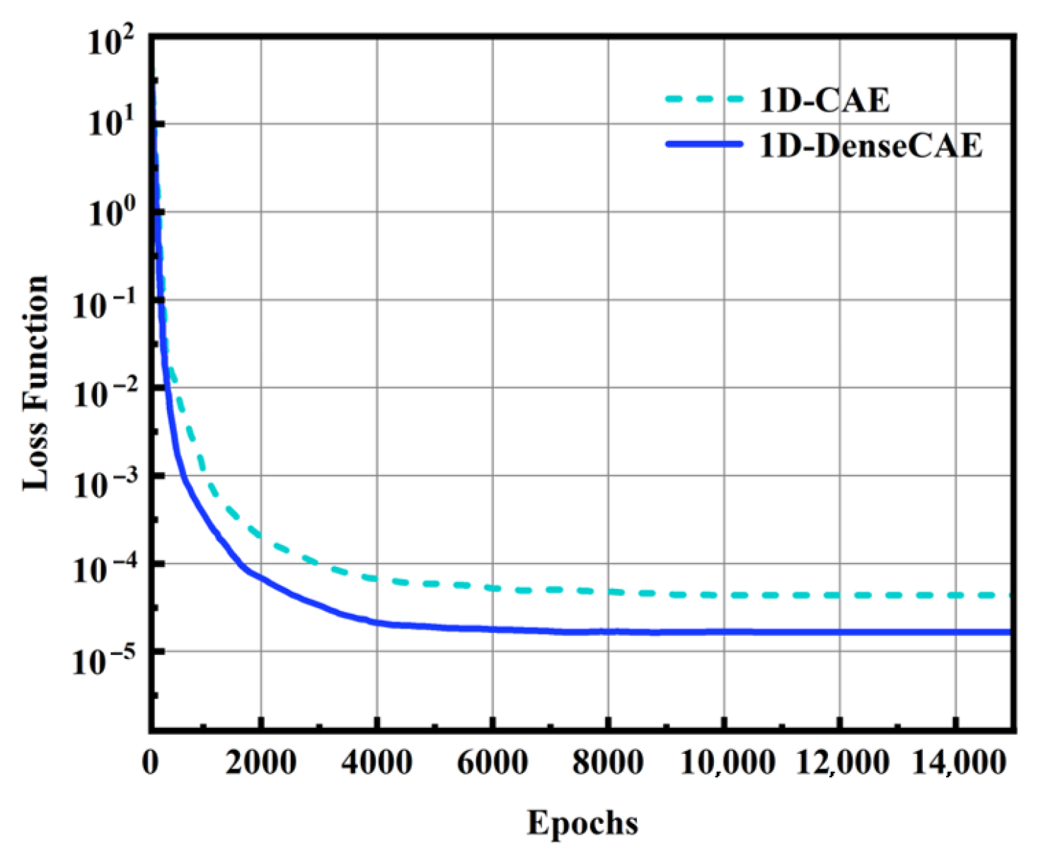
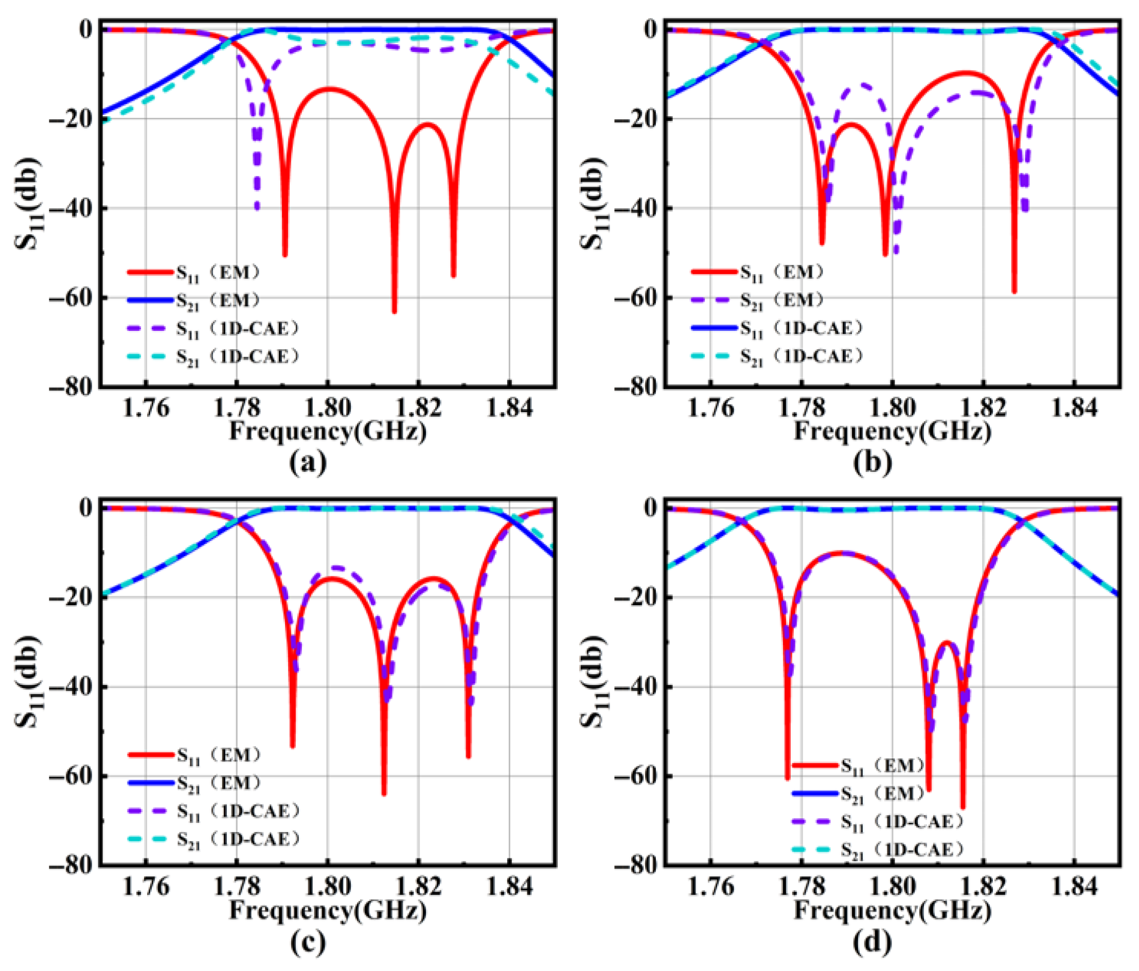
As shown in Figure 5, the loss decreases rapidly initially. The 1D-DenseCAE model’s loss stabilizes after around 6000 training iterations, approximately 25% faster than the 8000 iterations required by the traditional 1D-CAE model. This indicates that 1D-DenseCAE can more quickly identify an effective parameter space and adapt to the training data. Figure 6 and Figure 7 illustrate the training processes. The stabilized loss value of 1D-DenseCAE is significantly lower than that of 1D-CAE. Its fitting curve closely overlaps the simulation data, while the traditional model shows slight deviations even after 8000 iterations.

4.2. Verification of the Surrogate Model and IHOA

For verification, we selected two types of passband microwave filters as research samples. The first was an interdigital filter with a center frequency of   f 0 = 10   G H z , a passband from 8 to 12   GHz , and a requirement for S 11 below −20 dB within the passband, with in-band ripple under 0.5 dB. The second was a more complex seventh-order cross-coupled cavity filter with a center frequency of f 0 = 1.94   G H z , a passband from 1.92 to 1.96   GHz , and a requirement for S 11 below −20 dB within the passband, also with in-band ripple under 0.5 dB. These filters help evaluate the applicability and performance of optimization methods across different topological structures.
We designed a comprehensive data-driven optimization workflow, whose core lies in decoupling traditional time-consuming electromagnetic simulation tasks from intelligent agent models, thereby significantly enhancing optimization efficiency. First, a parameterizable 3D filter model was established in HFSS. Then, using the Python (3.13.5) automation interface (COM API) provided by HFSS, we controlled HFSS to perform batch simulations of different parameter combinations. For each set of geometric parameters, we extracted the corresponding S-parameters within their frequency range. After each simulation was completed, the system saved the geometric parameters (input) and the corresponding S-parameters (output) as a set of data samples, accumulating a total of 300 datasets. The data were stored in .csv format, forming the original training dataset for subsequent model learning. After the data preparation was complete, a proxy model was constructed and trained based on the 1D-DenseCAE structure. This model takes the geometric parameters of the filter as input and outputs the corresponding S-parameter spectrum. In the optimization phase, first, based on the S-parameters output by the proxy model, a fitness function was constructed that comprehensively considered design constraints such as center frequency, insertion loss, and in-band fluctuation. The function is as follows:
f x = m ax f [ f 1 , f 2 ] S 11 f , x 20 dB + λ i = 1 n x i x 0 2
Then, the IHOA was used to perform global search and local optimization of the filter structure parameters. After several iterations, the current optimal design was re-entered into HFSS for real simulation, and the results were added to the training set for incremental learning of the proxy model. This ensured the generalization ability of the proxy model while continuously improving its prediction accuracy in key design areas.

4.2.1. Verification of the Optimization Design of the Interdigital Filter Model

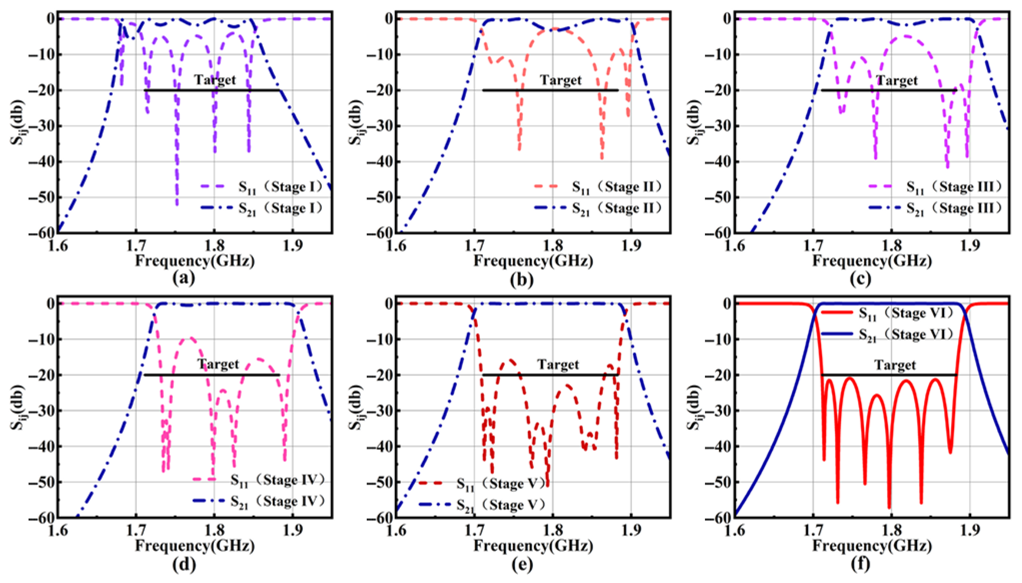
As shown in Figure 8, the interdigital filter model has geometric parameters H = h 1 , h 2 , h 3 , h 4 , h 5 T .
By adopting a surrogate model to replace repetitive simulations and combining it with a global–local collaborative optimization strategy, efficient searching was achieved. The S11 values of the filter were measured to be below −20 dB in the frequency range of 8 GHz to 12 GHz, thereby meeting the design target requirements. The optimized performance was significantly improved, as shown in Figure 9, and further verified by Table 2.

4.2.2. Verification of the Optimization Design of a Seventh-Order Cross-Coupled Cavity Filter

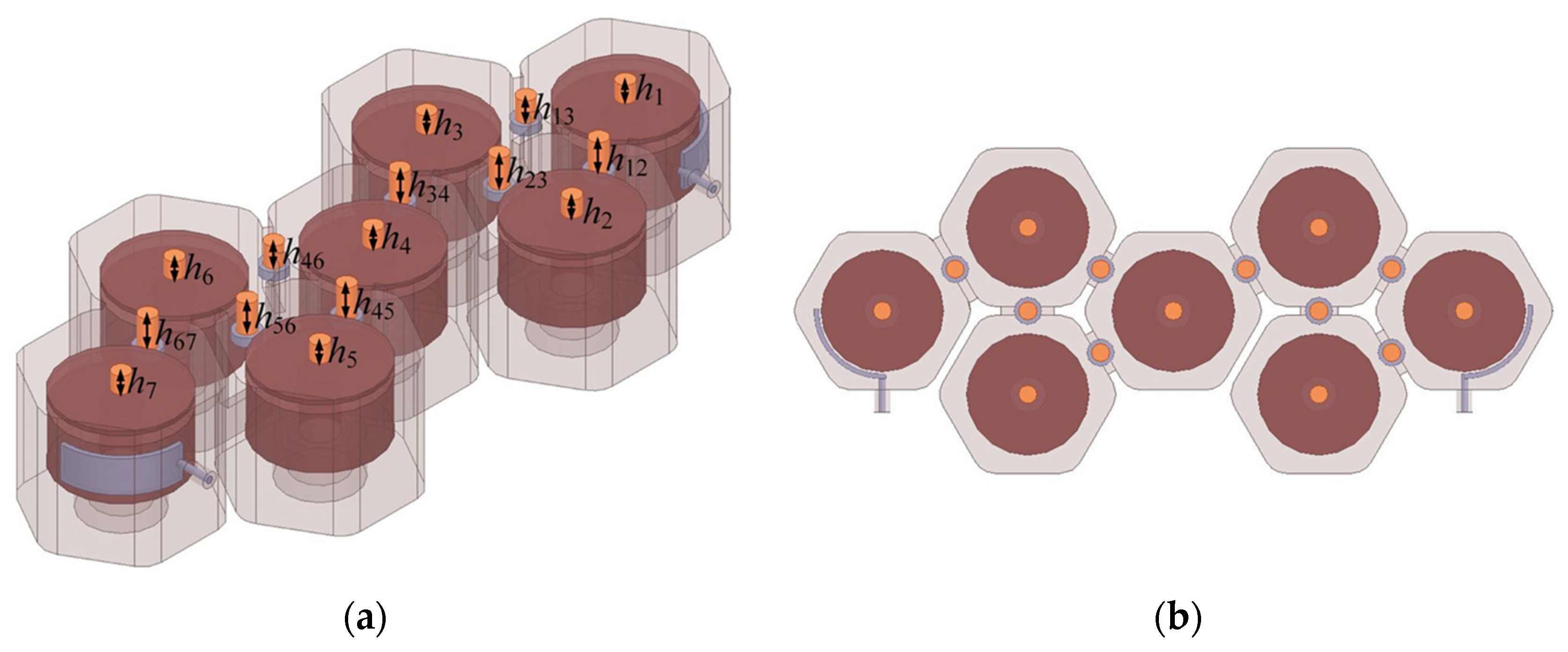
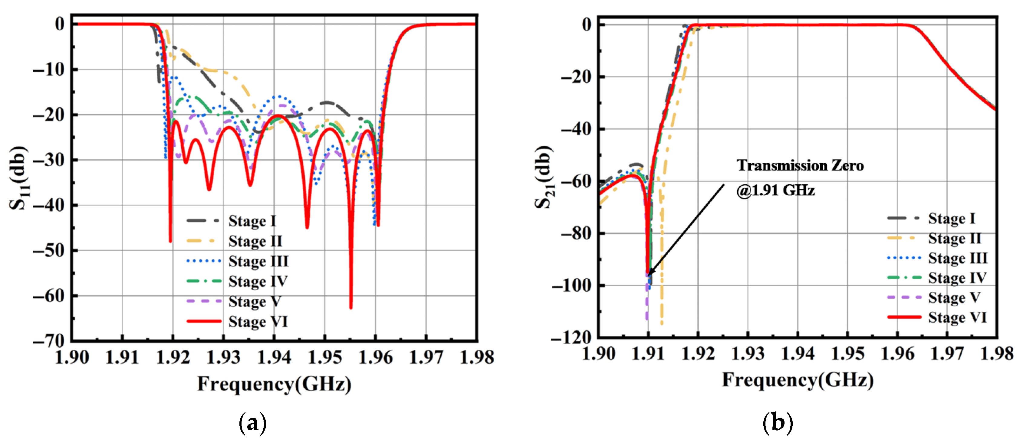
Figure 10 presents a complex seventh-order cross-coupled cavity filter. Its adjustable size parameters were H = h 1 , h 2 , h 3 , h 4 , h 5 , h 6 , h 7 , h 12 , h 23 , h 34 , h 45 , h 56 , h 67 , h 13 , h 46 T . Despite its complexity, the surrogate model could efficiently predict S-parameters using limited samples. Figure 11 shows the S-parameter responses obtained at different optimization stages using the IHOA. Table 3 lists the geometric design parameter values at each stage.
In optimizing the seventh-order cross-coupled cavity filter, the IHOA combined with the 1D-DenseCAE surrogate model performed remarkably. Over six iterations, key parameters like h1 converged from 3.75 mm to 3.967 mm (a fluctuation of ±5.7%), and h46 was fine-tuned from 5.175 mm to 5.166 mm (a change of <0.2%), highlighting the algorithm’s coordination of complex parameters. After optimization, the filter achieved better than −20 dB return loss ( S 11 ) within the passband from 1.92 to 1.96 GHz, indicating good impedance matching. A sharp transmission zero was observed at approximately 1.91 GHz, where the S 21 dropped to around −100 dB, effectively blocking signal transmission at that frequency. This deep null is attributed to the cross-coupling between non-adjacent resonators near the input side (between h1 and h3), which forms a signal cancellation path through destructive interference. The resulting improvement in out-of-band selectivity confirms the effectiveness of the cross-coupled topology in enhancing interference suppression. For high-dimensional, strongly coupled microwave filter structures, the IHOA efficiently achieves design goals using a limited number of samples.

5. Conclusions

This study proposes a solution driven by the 1D-DenseCAE surrogate model and IHOA. The 1D-DenseCAE enhances feature reuse via DenseNet, improving S-parameter prediction accuracy and training efficiency. It converges 25% faster compared to traditional 1D-CAE. In optimization, the IHOA shows high global exploration efficiency and meets strict design requirements (passband return loss below −20 dB, in-band ripple under 0.5 dB) in complex structures like interdigital filters and seventh-order cross-coupled cavity filters. This solution offers a reliable foundation for designing high-performance microwave filters.

Author Contributions

Conceptualization, S.G. and J.X.; methodology, L.Z.; software, L.Z.; validation, L.Z., J.X., and S.G.; formal analysis, L.Z.; investigation, L.Z.; resources, S.G.; data curation, S.G.; writing—original draft preparation, S.G.; writing—review and editing, J.X.; visualization, L.Z.; supervision, L.Z.; project administration, L.Z.; funding acquisition, L.Z. All authors have read and agreed to the published version of the manuscript.

Funding

This research was funded by the Natural Science Foundation of Inner Mongolia, grant number 2024MS05049.

Data Availability Statement

The original contributions presented in this study are included in the article. Further inquiries can be directed to the corresponding author.

Conflicts of Interest

The authors declare no conflicts of interest.

References

  1. Zhang, J.; Feng, F.; Jin, J.; Zhang, W.; Zhao, Z.; Zhang, Q.-J. Adaptively Weighted Yield-Driven EM Optimization Incorporating Neurotransfer Function Surrogate with Applications to Microwave Filters. IEEE Trans. Microw. Theory Tech. 2021, 69, 518–528. [Google Scholar] [CrossRef]
  2. Bandler, J.W.; Rayas-Sánchez, J.E.; Zhang, Q.-J. Yield-driven electromagnetic optimization via space mapping-based neuromodels. Int. J. RF Microw. Comput.-Aided Eng. 2002, 12, 79–89. [Google Scholar] [CrossRef]
  3. Zhang, J.; Feng, F.; Na, W.; Yan, S.; Zhang, Q. Parallel Space-Mapping Based Yield-Driven EM Optimization Incorporating Trust Region Algorithm and Polynomial Chaos Expansion. IEEE Access 2019, 7, 143673–143683. [Google Scholar] [CrossRef]
  4. Pietrenko-Dabrowska, A. Rapidtolerance-awaredesign of miniaturized microwave passives by means ofconfined-domainsurrogates. Int. J. Numer. Model. Electron. Netw. Devices Fields 2020, 33, e2779. [Google Scholar] [CrossRef]
  5. Koziel, S.; Bekasiewicz, A. Sequential approximate optimisation for statistical analysis and yield optimisation of circularly polarised antennas. IET Microw. Antennas Propag. 2018, 12, 2060–2064. [Google Scholar] [CrossRef]
  6. Ciccazzo, A.; Di Pillo, G.; Latorre, V. A SVM Surrogate Model-Based Method for Parametric Yield Optimization. IEEE Trans. Comput.-Aided Des. Integr. Circuits Syst. 2016, 35, 1224–1228. [Google Scholar] [CrossRef]
  7. Bo, L.; Qingfu, Z.; Fernández, F.V.; Gielen, G. An Efficient Evolutionary Algorithm for Chance-constrained Bi- objective Stochastic Optimization. IEEE Trans. Evol. Comput. 2013, 17, 786–796. [Google Scholar] [CrossRef]
  8. Jin, J.; Feng, F.; Na, W.; Zhang, J.; Zhang, W.; Zhao, Z.; Zhang, Q.-J. Advanced Cognition-Driven EM Optimization Incorporating Transfer Function-Based Feature Surrogate for Microwave Filters. IEEE Trans. Microw. Theory Tech. 2021, 69, 15–28. [Google Scholar] [CrossRef]
  9. Zhao, P.; Wu, K. Homotopy Optimization of Microwave and Millimeter-Wave Filters Based on Neural Network Model. IEEE Trans. Microw. Theory Tech. 2020, 68, 1390–1400. [Google Scholar] [CrossRef]
  10. Xue, L.; Liu, B.; Yu, Y.; Cheng, Q.S.; Imran, M.; Qiao, T. An Unsupervised Microwave Filter Design Optimization Method Based on a Hybrid Surrogate Model-Assisted Evolutionary Algorithm. IEEE Trans. Microw. Theory Tech. 2023, 71, 1159–1170. [Google Scholar] [CrossRef]
  11. Yu, Y.; Zhang, Z.; Cheng, Q.S.; Liu, B.; Wang, Y.; Guo, C.; Ye, T.T. State-of-the-Art: AI-Assisted Surrogate Modeling and Optimization for Microwave Filters. IEEE Trans. Microw. Theory Tech. 2022, 70, 4635–4651. [Google Scholar] [CrossRef]
  12. Zhang, Z.; Liu, B.; Yu, Y.; Imran, M.; Cheng, Q.S.; Yu, M. A Surrogate Modeling Space Definition Method for Efficient Filter Yield Optimization. IEEE Microw. Wirel. Technol. Lett. 2023, 33, 631–634. [Google Scholar] [CrossRef]
  13. Zhang, Z.; Liu, B.; Yu, Y.; Cheng, Q.S. A Microwave Filter Yield Optimization Method Based on Off-Line Surrogate Model-Assisted Evolutionary Algorithm. IEEE Trans. Microw. Theory Tech. 2022, 70, 2925–2934. [Google Scholar] [CrossRef]
  14. Zhao, W.-S.; Wang, B.-X.; Wang, D.-W.; You, B.; Liu, Q.; Wang, G. Swarm Intelligence Algorithm-Based Optimal Design of Microwave Microfluidic Sensors. IEEE Trans. Ind. Electron. 2022, 69, 2077–2087. [Google Scholar] [CrossRef]
  15. Liang, S.; Fang, Z.; Sun, G.; Qu, G. Biogeography-based optimization with adaptive migration and adaptive mutation with its application in sidelobe reduction of antenna arrays. Appl. Soft Comput. 2022, 121, 108772. [Google Scholar] [CrossRef]
  16. Koziel, S.; Pietrenko-Dabrowska, A. Efficient Simulation-Based Global Antenna Optimization Using Characteristic Point Method and Nature-Inspired Metaheuristics. IEEE Trans. Antennas Propag. 2024, 72, 3706–3717. [Google Scholar] [CrossRef]
  17. Ghasemi, M.; Zare, M.; Trojovský, P.; Rao, R.V.; Trojovská, E.; Kandasamy, V. Optimization based on the smart behavior of plants with its engineering applications: Ivy algorithm. Knowl.-Based Syst. 2024, 295, 111850. [Google Scholar] [CrossRef]
  18. Oladejo, S.O.; Ekwe, S.O.; Mirjalili, S. The Hiking Optimization Algorithm: A novel human-based metaheuristic approach. Knowl. -Based Syst. 2024, 296, 111880. [Google Scholar] [CrossRef]
  19. Hou, Y.; Wu, Z.; Cai, X.; Zhu, T. The application of improved densenet algorithm in accurate image recognition. Sci. Rep. 2024, 14, 8645. [Google Scholar] [CrossRef]
  20. Rayas-Sanchez, J.E.; Gutierrez-Ayala, V. EM-Based Monte Carlo Analysis and Yield Prediction of Microwave Circuits Using Linear-Input Neural-Output Space Mapping. IEEE Trans. Microw. Theory Tech. 2006, 54, 4528–4537. [Google Scholar] [CrossRef]
  21. Sabbagh, M.A.E.; Bakr, M.H.; Bandler, J.W. Adjoint higher order sensitivities for fast full-wave optimization of microwave filters. IEEE Trans. Microw. Theory Tech. 2006, 54, 3339–3351. [Google Scholar] [CrossRef]
  22. Ochoa, J.S.; Cangellaris, A.C. Random-Space Dimensionality Reduction for Expedient Yield Estimation of Passive Microwave Structures. IEEE Trans. Microw. Theory Tech. 2013, 61, 4313–4321. [Google Scholar] [CrossRef]
  23. Koziel, S.; Bandler, J.W. Rapid Yield Estimation and Optimization of Microwave Structures Exploiting Feature-Based Statistical Analysis. IEEE Trans. Microw. Theory Tech. 2015, 63, 107–114. [Google Scholar] [CrossRef]
  24. Du, B.; Xiong, W.; Wu, J.; Zhang, L.; Zhang, L.; Tao, D. Stacked Convolutional Denoising Auto-Encoders for Feature Representation. IEEE Trans. Cybern. 2017, 47, 1017–1027. [Google Scholar] [CrossRef]
  25. Mondal, A.; Shrivastava, V.K. A novel Parametric Flatten-p Mish activation function based deep CNN model for brain tumor classification. Comput. Biol. Med. 2022, 150, 106183. [Google Scholar] [CrossRef]
  26. Sheikholeslami, R.; Razavi, S. Progressive Latin Hypercube Sampling: An efficient approach for robust sampling-based analysis of environmental models. Environ. Model. Softw. 2017, 93, 109–126. [Google Scholar] [CrossRef]
  27. Goodwin, A.; Hammett, M.; Harris, M. The application of Tobler’s hiking function in data-driven traverse modelling for planetary exploration. Acta Astronaut. 2025, 228, 265–273. [Google Scholar] [CrossRef]
  28. Wyka, T.P. Negative phototropism of the shoots helps temperate liana Hedera helix L. to locate host trees under habitat conditions. Tree Physiol. 2023, 43, 1874–1885. [Google Scholar] [CrossRef]
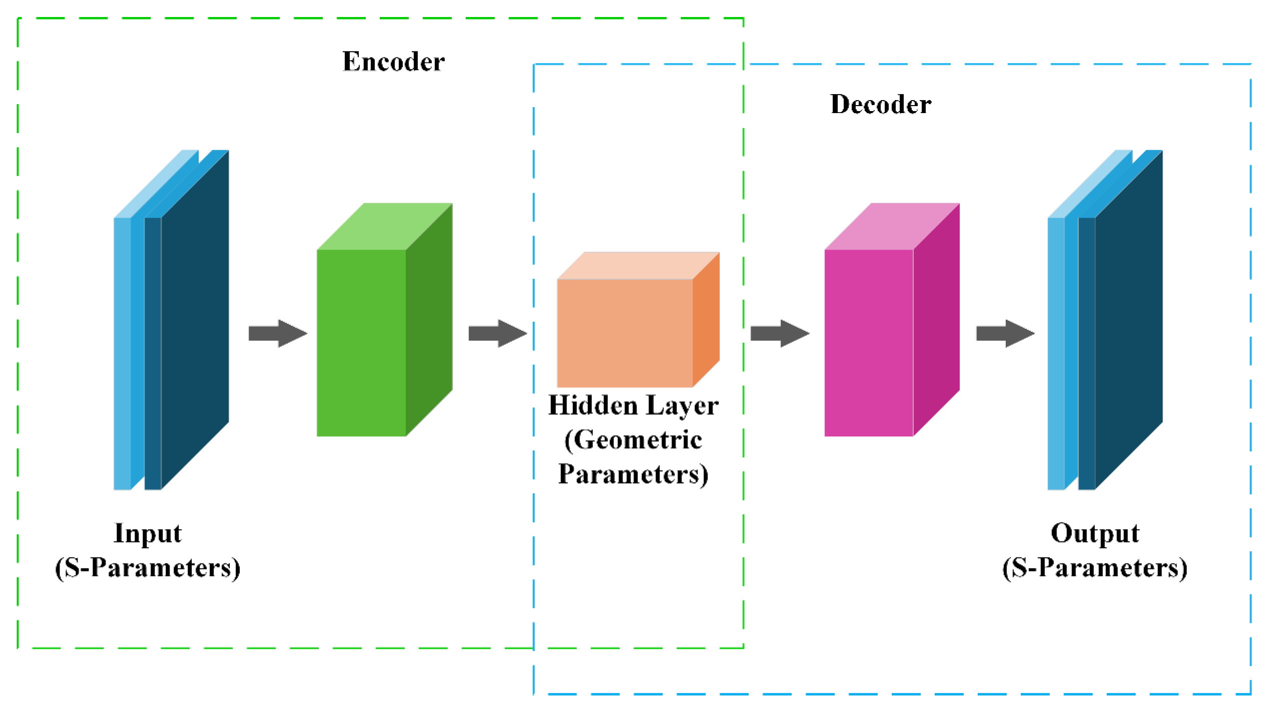
Figure 1. Architecture of the 1D-DenseCAE surrogate model.
Electronics 14 03305 g001
Figure 2. Architecture of the 1D-DenseCAE model.
Electronics 14 03305 g002
Figure 3. Filter design process based on the 1D-DenseCAE model and IHOA.
Electronics 14 03305 g003
Figure 4. (a) Perspective view of the cavity filter; (b) top view of the cavity filter.
Electronics 14 03305 g004
Figure 5. Curve of loss values during network training.
Electronics 14 03305 g005
Figure 6. Training process of 1D-DenseCAE: (a) 2000 iterations; (b) 4000 iterations; (c) 6000 iterations.
Electronics 14 03305 g006
Figure 7. Training process of 1D-CAE: (a) 2000 iterations; (b) 4000 iterations; (c) 6000 iterations; (d) 8000 iterations.
Electronics 14 03305 g007
Figure 8. (a) Perspective view of the interdigital filter; (b) top view of the interdigital filter.
Electronics 14 03305 g008
Figure 9. S-parameters corresponding to each stage: (a) Stage 1; (b) Stage 2; (c) Stage 3; (d) Stage 4; (e) Stage 5; (f) Stage 6.
Electronics 14 03305 g009
Figure 10. Seventh-order cross-coupled cavity filter: (a) perspective view; (b) top view.
Electronics 14 03305 g010
Figure 11. S-parameters corresponding to each stage: (a) S 11 ; (b) S 21 .
Electronics 14 03305 g011
Table 1. Network parameter settings of the 1D-DenseCAE model.
LayerSize/NodesStrideOutput ShapeActivation
Input Layer[400, 2]-[400, 2]-
Encoder
Initial Conv Layer3 × 161[400, 16]-
Dense Block 1Conv13 × 121[400, 28]ReLU
Conv23 × 121[400, 40]ReLU
Conv33 × 121[400, 52]ReLU
Conv43 × 121[400, 64]ReLU
Transition Layer 11 × 242[200, 32]ReLU
Dense Block 2Conv13 × 121[200, 32]ReLU
Conv23 × 121[200, 44]ReLU
Conv33 × 121[200, 56]ReLU
Conv43 × 121[200, 68]ReLU
Transition Layer 21 × 482[100, 40]ReLU
Dense Block 3Conv13 × 121[100, 52]ReLU
Conv23 × 121[100, 64]ReLU
Conv33 × 121[100, 76]ReLU
Conv43 × 121[100, 88]ReLU
Transition Layer 31 × 482[50, 44]ReLU
Flatten Layer2200-[2200]-
Decoder
Fully Connected Layer 1256 Nodes-[256]Mish
Fully Connected Layer 21024 Nodes-[1024]Mish
Fully Connected Layer 3800 Nodes-[800]Mish
Reshape Layer--[400, 2]-
Table 2. Values of the geometric design parameters for each stage.
Stage 1Stage 2Stage 3Stage 4Stage 5Stage 6
h10.3290.4180.3780.2590.2880.274
h21.6741.5931.7331.6311.6531.642
h31.8381.6771.7181.8121.8341.805
h41.6781.6981.6711.7341.7531.779
h51.6281.5831.7941.8221.7971.806
Table 3. Values of the geometric design parameters for each stage.
Stage 1Stage 2Stage 3Stage 4Stage 5Stage 6
h13.753.9244.1134.0743.9263.967
h23.8464.1794.1883.9894.1254.146
h33.8264.1733.8854.2494.1764.118
h43.7513.7474.2583.9224.0664.05
h53.9453.993.7124.1374.0523.997
h64.0253.8943.7764.0334.2593.839
h73.9664.2143.7893.7533.9444.059
h126.83176.7166.9516.866.969
h237.2577.0297.0497.0847.1047.289
h347.2556.9457.1337.0296.9897.021
h456.7946.8736.7287.2057.1417.148
h567.0937.17.2977.0287.0336.97
h676.9247.2697.0777.1597.1897.276
h135.134.8764.7025.055.0324.948
h465.1754.7364.7924.9375.1015.166
Disclaimer/Publisher’s Note: The statements, opinions and data contained in all publications are solely those of the individual author(s) and contributor(s) and not of MDPI and/or the editor(s). MDPI and/or the editor(s) disclaim responsibility for any injury to people or property resulting from any ideas, methods, instructions or products referred to in the content.