Multi-Criteria Visual Quality Control Algorithm for Selected Technological Processes Designed for Budget IIoT Edge Devices

Abstract

This paper presents an innovative multi-criteria visual quality control algorithm designed for deployment on cost-effective Edge devices within the Industrial Internet of Things environment. Traditional industrial vision systems are typically associated with high acquisition, implementation, and maintenance costs. The proposed solution addresses the need to reduce these costs while maintaining high defect detection efficiency. The developed algorithm largely eliminates the need for time- and energy-intensive neural network training or retraining, though these capabilities remain optional. Consequently, the reliance on human labor, particularly for tasks such as manual data labeling, has been significantly reduced. The algorithm is optimized to run on low-power computing units typical of budget industrial computers, making it a viable alternative to server- or cloud-based solutions. The system supports flexible integration with existing industrial automation infrastructure, but it can also be deployed at manual workstations. The algorithm’s primary application is to assess the spread quality of thick liquid mold filling; however, its effectiveness has also been demonstrated for 3D printing processes. The proposed hybrid algorithm combines three approaches: (1) the classical SSIM image quality metric, (2) depth image measurement using Intel MiDaS technology combined with analysis of depth map visualizations and histogram analysis, and (3) feature extraction using selected artificial intelligence models based on the OpenCLIP framework and publicly available pretrained models. This combination allows the individual methods to compensate for each other’s limitations, resulting in improved defect detection performance. The use of hybrid metrics in defective sample selection has been shown to yield superior algorithmic performance compared to the application of individual methods independently. Experimental tests confirmed the high effectiveness and practical applicability of the proposed solution, preserving low hardware requirements.

1. Introduction

Vision systems in industrial processes offer significantly greater effectiveness and efficiency compared to manual inspection [1], aligning with the evolving Edge Computing solutions in IIoT [2]. One of their key applications is the automatic verification of proper filling of containers with liquids, bulk materials, and similar substances. These systems serve as an alternative to traditional distance sensors, especially in small containers where traditional sensors fail [3]. A common solution involves a single-point distance sensor, often used to measure liquid levels in tanks. However, this approach has limitations, especially when dealing with liquids that exhibit poor flow properties (e.g., thick, viscous, or foaming), which can lead to surface irregularities such as waves, swirls, bubbles, or sediment. An accurate measurement requires the liquid to have good flow characteristics. In multi-point measurement systems, the installation of multiple sensors increases system complexity and cost, due to the need for calibration, maintenance, data integration, and communication management. A more efficient alternative is the use of RGB-D (Red, Green, Blue, and Depth) cameras, although their implementation is not always economically viable. The RGB-D cameras generate large volumes of data, requiring substantial computational resources—typically provided by High-performance Computing (HPC) units or cloud-based infrastructures. The high cost of such solutions often excludes them from low-budget applications. The RGB-D and stereovision systems are appreciated for their high precision and widespread use in spatial analysis and the detection of geometric deviations. Their deployment, however, necessitates the acquisition of specialized, often costly, hardware and a meticulous calibration process using reference objects [4,5]. A cost-effective alternative lies in monocular methods, which estimate depth from a single image and permit a simplified calibration using the coordinates of a reference object. The measuring accuracy of these methods is significantly constrained by a higher measurement error when compared to hardware-based solutions, particularly when absolute depth values are required. Consequently, in industrial environments, where the primary goal is the detection of relative geometric deviations and shape deformations, relative depth measurement (rather than absolute) emerges as an effective compromise. This approach enables the identification of changes in an object’s position and geometry despite a lower metric precision. This conclusion is supported by calibration problems and their influence on the accuracy described in the literature related to industrial deployments and the accuracy assessment of various depth sensors [6].

An alternative approach involves low-cost industrial setups, where an industrial camera performs measurements and data is processed locally, adhering to Edge Computing principles—one of the pillars of the Industrial Internet of Things (IIoT) [7]. Moving processing closer to the production line not only improves system responsiveness but also enhances both functional safety and cybersecurity. Edge processing reduces latency, which is critical for real-time safety operations, and keeps data on-site, minimizing exposure to external threats.

Within the domain of vision-based quality control, classifiers are used to detect defects in processes, based on both classical descriptors (based on hand-crafted features) and Artificial Intelligence (AI) systems. The AI-based systems are considerably more flexible in many applications. In classical systems, a major challenge involves precisely tuning vision methods to the specific characteristics and dynamics of the 2D/3D scene. In this context, approaches such as transfer learning and zero-shot learning (e.g., YOLO—You Only Look Once) are particularly relevant.

In the context of product evaluation, where an image of a reference (ideal) product is compared with an image of an actual product from the production line, seven key application areas can be distinguished:

• Objective and Quantitative Quality Assessment—Unlike subjective visual inspection by humans, vision-based quality indicators provide objective and measurable values. This enables precise determination of product conformity with the reference and automatic detection of deviations.
• Automation of Quality Control—Images of successive products are compared with the reference, and vision-based quality indicators allow for automatic classification of products as compliant or non-compliant. This eliminates human error, increases inspection speed, and reduces control costs.
• Detection of Subtle Defects—Vision techniques can detect subtle differences in images that may be difficult for the human eye to notice, especially during prolonged and monotonous inspection processes. This includes minor discolorations, surface imperfections, texture changes, or print irregularities.
• Monitoring of Production Process Stability—Frequent measurements of products coming off the production line allow for monitoring the stability of the process. Sudden changes in vision-based quality indicators and trend analysis may signal issues in the production process.
• Documentation and Trend Analysis—Recording the results of visual inspections creates a valuable dataset. This enables analysis of product quality trends over time, identification of recurring issues, and informed decision-making for process optimization.
• Reduction of Waste and Efficiency Improvement—Early detection of defective products using these indicators minimizes material and energy losses. Non-compliant products can be rejected at an early stage, before undergoing further costly processing.
• Ensuring Quality Consistency—In industrial applications where visual consistency is critical (e.g., decorative elements, packaging, or electronic components), reference image quality indicators ensure that each produced item meets the established standard.

This study focuses on the multi-criteria visual quality control algorithm for selected technological processes designed for budget IIoT Edge devices. It presents a hybrid solution that leverages the individual strengths of various methods to achieve greater efficiency and effectiveness than when used independently. The hardware foundation of budget Edge processing systems is based on energy-efficient industrial computers or embedded system platforms, typically with limited computational power. It stands in contrast to systems that have migrated from external cloud environments to the local enterprise domain [8], driven by cybersecurity concerns [9], network Quality of Service (QoS) limitations, and other operational factors. While this migration provides access to local HPC resources (including on-premises cloud solutions), the high cost of deployment and maintenance makes it economically unjustifiable to use them for implementing a single functionality, such as a vision-based quality control algorithm.

Notably, the development of highly efficient and lightweight algorithms for budget systems, combined with optimization, also allows their use as auxiliary processes in high-performance Edge systems [10]. Their architecture, adapted for parallel computing, ensures that such integration does not significantly burden these systems [9].

2. Vision-Based Monitoring and Quality Control Station in Industrial Processes

The vision-based monitoring and quality control station is installed above the product collection point. The collection of the inspected objects may be performed manually or automatically and is the final step in processes such as filling a container with liquid, dispensing bulk material, or packing multiple identical objects into a container. The camera is mounted in a fixed position, and the object is mechanically positioned under the camera in the same location for each measurement. The scene in which the object is placed is neither additionally illuminated nor enclosed. Although the term product is used throughout this description, it does not necessarily refer to a final product. It may also denote the outcome of a completed stage within the production process. A commonly used approach in such systems is comparative analysis between the current product and a previously recorded reference. However, this method may be problematic in cases involving short, one-time production series, high variability, or frequent product rotation. Due to time constraints, these processes rarely permit the construction of a dependable evaluation baseline. High product variability forces continuous re-referencing, which is time-consuming and error-prone. A simplified approach involves registering the first object in a series (or the one identified manually as optimal during system startup) as the reference, and then monitoring deviations between subsequent objects over time. Although less precise than classical methods, this approach enables a quick start to quality control and can detect deviations without complex configuration. This is a practical compromise for some short production runs.

This approach to quality control is intended to detect defects without classifying their reasons related to:

• clogging of pumps, presses, feeders, or chutes,
• overfilling or underfilling, spillage, and other similar issues,
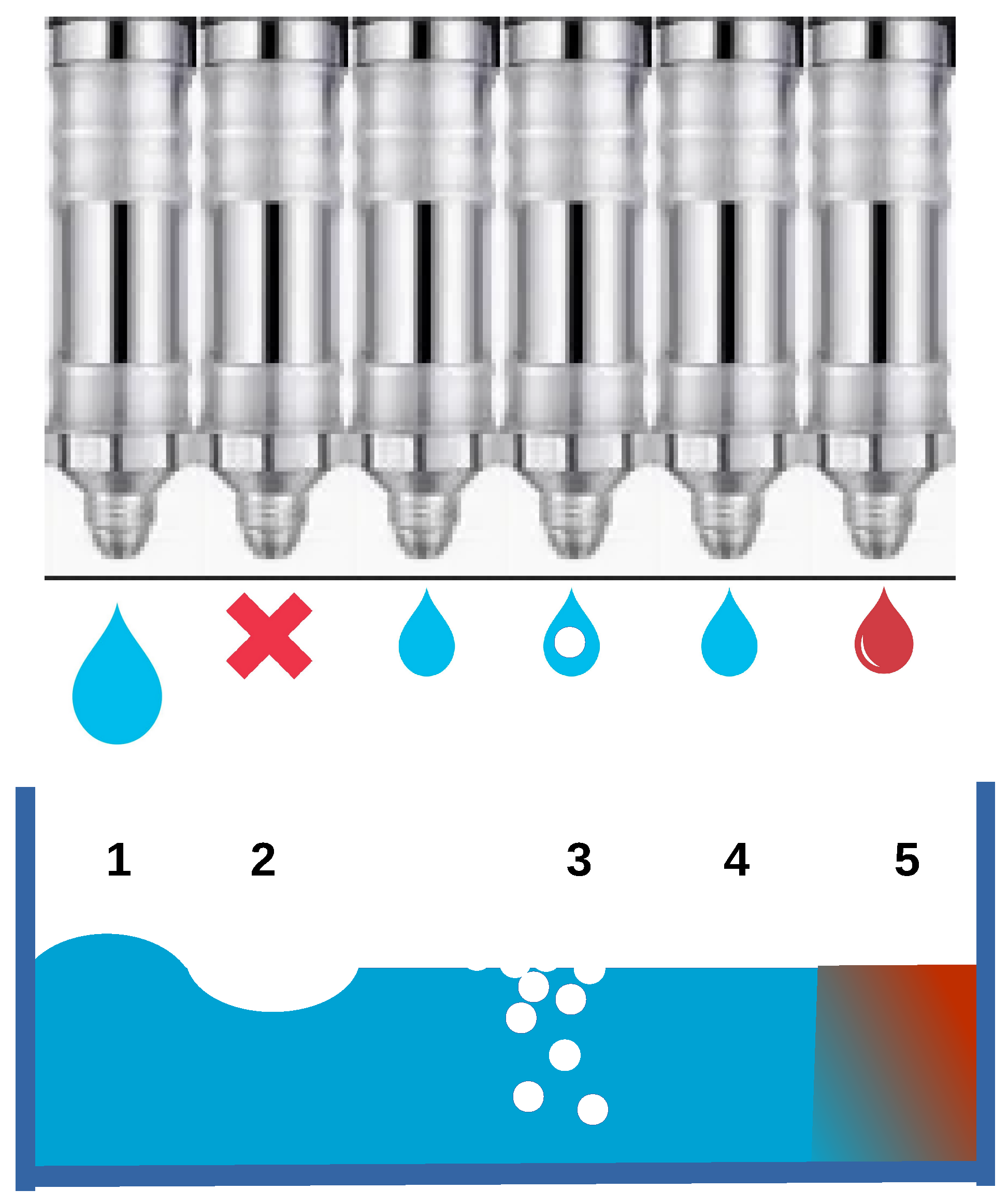
• changes in the physical properties of the substances deposited in containers (e.g., incorrect viscosity, density, altered flow ability, Figure 1, or clumping).

Additionally, the system should ensure that the product maintains a consistent level within predefined, non-negotiable quality limits over time. A representative example illustrating this issue is the process of automatic filling of cake molds, where the collection point in the technological process corresponds to the physical transfer of the dough to the baking oven. The dough, dispensed by pumps or presses, spreads across the mold under gravity. During dough preparation, parameters affecting its flow behavior may change, and it is, for example, unacceptable for empty spaces to form in the mold corners. The spreading process may also be assisted by mold movement. In such cases, the vision-based quality control system can indirectly detect uneven mold movement. It is also unacceptable, especially in systems with multiple dough dispensing points (optionally with a moving mold), for wave-like patterns to form. Common defects in dense liquid container filling processes are shown in Figure 1. It illustrates typical problems encountered during automatic filling of molds with viscous liquids (e.g., cake batter): (1) excessive flow resulting in convex surface formations and overflow; (2) clogged nozzle causing insufficient flow and visible concave depressions; (3) aeration effects leading to texture changes, foam formation, and surface irregularities; (5) contamination or dye staining causing unexpected coloration and surface discoloration. These defects represent the primary quality control challenges that the proposed vision-based system is designed to detect. The point (4) refers to the correct filling condition, which ensures a uniform surface level and appropriate distribution.

The automated quality control system is designed to replace human operators, who are often responsible for both inspection and product handling. As a result, the quality of manual inspection tends to decline over time due to operator fatigue. The system is primarily designed to provide an objective and quantitative assessment of product quality, verifiable through standardized metrics, as well as to enable monitoring of production process stability.

3. Evaluation Criteria and Computational Constraints in Budget IIoT Edge Systems

In the proposed system, two key quality control factors are considered: overall visual similarity between the current product and a reference model, and the geometric parameters of the object, indirectly monitored through depth maps extracted from the image.

Adhering to the design principles of a cost-effective architecture, the selection of algorithms was guided by the requirement for low computational complexity. All tests were conducted on hardware platforms representative of budget-friendly Edge Computing devices for Industrial Internet of Things (IIoT) applications, with comparable acquisition costs: the Jetson Orin Nano and an industrial PC equipped with an Intel Celeron processor. The Jetson Orin Nano, a platform developed by NVIDIA, features the Ampere architecture with 1024 NVIDIA CUDA cores, 32 Tensor cores, and a 6-core Arm® Cortex-A78AE v8.2 64-bit CPU, along with 4 GB of 128-bit LPDDR5 memory. It offers excellent support for AI-based applications [11], facilitated by NVIDIA’s development ecosystem. The industrial PC, powered by an Intel Celeron J6412 processor (2.6 GHz max, 4 cores, 4 threads), 8 GB DDR RAM, and Intel UHD Graphics, may be considered a less powerful alternative to the Jetson Nano series due to the lack of hardware acceleration (no CUDA or Tensor cores). However, Intel processors benefit from the highly optimized OpenVINO^TM toolkit, which supports the deployment of AI applications [12].

Despite advances in lightweight defect detection models, such as MobileNetV2-based defect detectors and optimized YOLO variants [13,14], which demonstrate impressive performance, they require infrastructure investments and training procedures that exceed the operational constraints of small-scale food production environments. MobileNet-based solutions, despite achieving high accuracy, still necessitate extensive labeled datasets and GPU-accelerated training. Similarly, self-supervised anomaly detection methods [15,16], while reducing labeling requirements, demand substantial computational resources for contrastive learning phases. The presented approach prioritizes immediate deployability using established components over algorithmic sophistication, addressing the specific economic and operational constraints of a small food manufacturer. The selection of relatively simple and well-established methods such as SSIM, MiDaS, and OpenCLIP is a deliberate design decision. This choice reflects the practical constraints of small-scale industrial environments, where production variability, limited data availability, and cost-sensitive deployment timelines make complex, data-driven solutions impractical. The proposed algorithm prioritizes robustness, ease of implementation, and low computational burden, enabling rapid deployment without the need for extensive training or calibration. While more advanced techniques, such as adaptive weighting or rule learning, are acknowledged and discussed as future directions, the proposed approach offers a pragmatic balance between performance and feasibility.

3.1. Visual Similarity Assessment Using SSIM

To evaluate image similarity, the Structural SIMilarity index (SSIM) [17] is employed as a representative full-reference image quality metric. Among known image quality assessment (IQA) methods [18], the SSIM is considered one of the most intuitive and practical, as it aligns well with human visual perception, more accurately reflecting what a human observer would perceive as a “difference” between images. The SSIM compares two images based on three key components: luminance, contrast, and structure, by analyzing local pixel patterns such as edges and textures. It is relatively insensitive to uniform changes in brightness or contrast, which typically do not significantly affect perceived image quality. Instead, it focuses on structural distortions, which are more noticeable to the human eye. Within the system, this indicator is responsible for detecting changes in luminance, contrast, and structure in areas of the image that are expected to remain visually consistent, such as flat or homogeneous surfaces. The assessment is widely implemented, offering optimized code, numerical stability, and a standardized scale, which facilitates the definition of acceptance thresholds in automated quality control systems. The Python 3.12 implementation is available via the scikit-image [19] and the PyIQA library [20].

In real-time quality control systems, the implementation is sufficiently fast for most applications. The computational cost is acceptable considering the provided diagnostic value compared to simpler metrics.

Limitations of SSIM

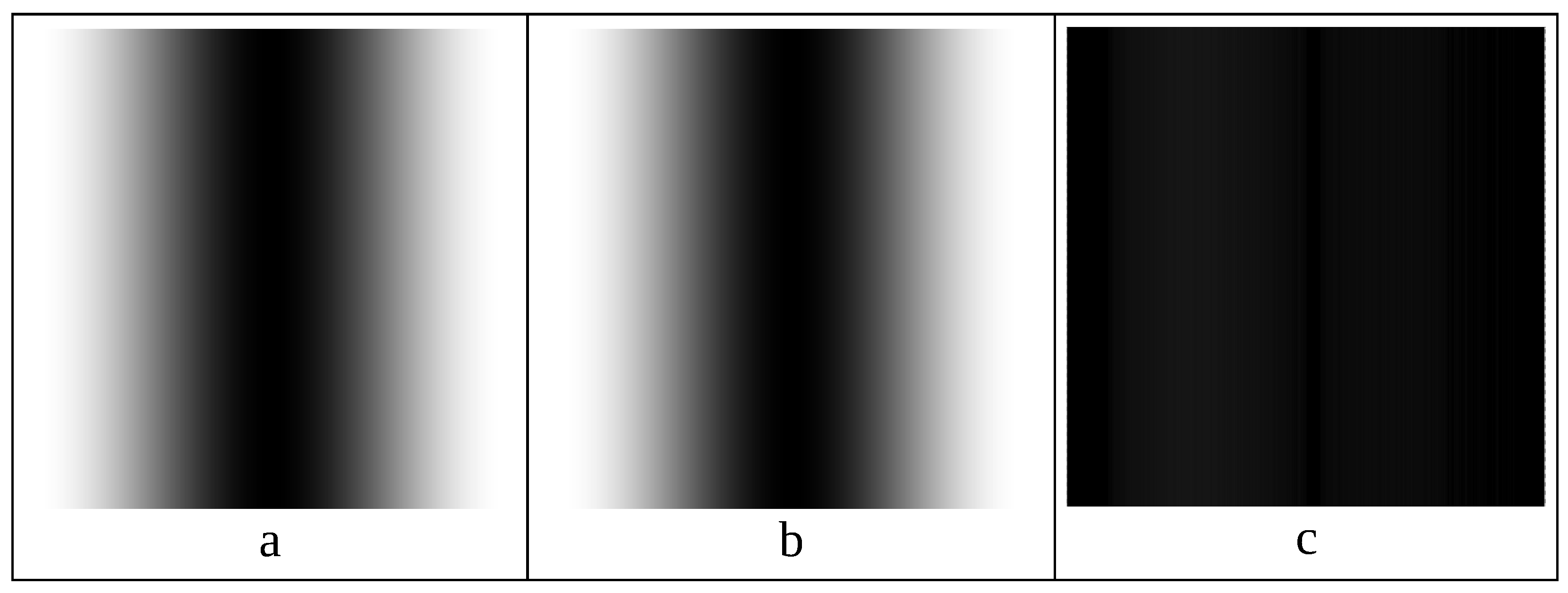
SSIM has certain limitations; Figure 2 illustrates a case in which SSIM indicates a high degree of similarity (SSIM = 0.9999) between two images. The images visualize the surfaces of 3D cylindrical objects that differ in diameter by 10%. This discrepancy is not easily noticeable to the human eye, which would likely perceive the images as nearly identical. To highlight the differences between images a and b, a differential image is provided (denoted as c in Figure 2). The example has been synthetically generated to emphasize this limitation; however, similar situations may also occur in real-world imagery.

3.2. The Role of Depth Maps

This paper proposes an algorithm for an inspection station where images have been acquired using a single-lens camera. This setup necessitates depth estimation without relying on stereo vision techniques or RGB-D cameras. Depth maps were generated using the Intel MiDaS v2.1 (Monocular Depth Estimation via a Multi-Scale Vision Transformer) framework [21]. The Intel MiDaS framework is a deep learning model [21,22,23,24] designed to estimate relative depth from a single RGB image. It has numerous practical deployments and a rich repository of example codes. Pretrained models are also available. This technology predicts spatial relationships, i.e., it determines which objects are closer or farther away, and thus operates on arbitrary images without requiring camera calibration. The available models were trained on diverse image datasets, enhancing their generalization capabilities. Furthermore, thanks to zero-shot transfer learning, the model performs well even on previously unseen data. MiDaS version 3 was not used due to its higher hardware requirements compared to version 2.1. The OpenVINO^TM technology support is no longer provided for version 3. The experiment employed the MiDaS Large DPT model available via the PyTorch version 2.8 Hub repository. MiDaS version 3 models, particularly those based on transformer architectures such as ViT, BEiT, and Swin, generally exhibit significantly higher computational and memory demands. While these models offer improved prediction accuracy, their increased size and architectural complexity can lead to substantial performance degradation or even render them inoperable on resource-constrained platforms such as the Jetson Nano. Consequently, MiDaS version 2.1 emerges as a more practical choice for applications where real-time performance is a critical requirement. Alternative methods for generating depth maps from images are also available based on artificial intelligence, as are methods for measuring the similarity of depth maps [25,26,27].

To compare depth maps, a histogram is computed for each map, followed by the calculation of the normalized Manhattan Distance (also known as City Block Distance, Taxicab Distance, or L1 Norm) [28]. This metric measures the sum of absolute differences between the coordinates of corresponding points in a multidimensional space. In practice, it is implemented using the SciPy library in Python, as demonstrated in the example code shown in Figure 3.

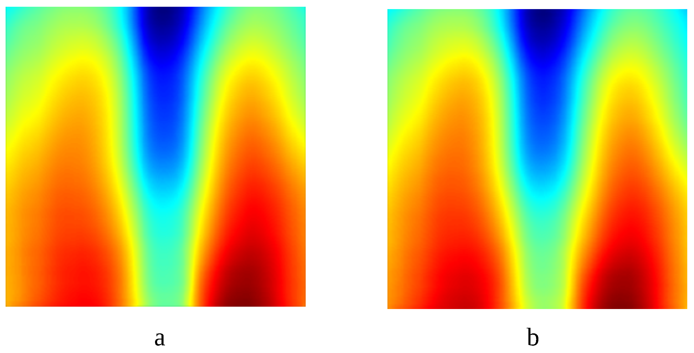
To resolve the SSIM-related issue described earlier, involving visually similar but geometrically different cylinders, MiDaS-based depth map estimation was applied (Figure 4). In contrast to SSIM, the cityblock_histogram_similarity value for the corresponding depth maps is lower, at 0.9531, indicating a discrepancy in geometric structure. For brevity, this metric will be referred to as Cityblock throughout the remainder of this paper. In this context, depth map analysis not only mitigates the limitations of SSIM but also provides an indirect means of assessing geometric properties of the scene and its objects.

Limitations of Monocular Depth Estimation and Mitigation Strategies

Despite its advantages, MiDaS technology for estimating depth on images has certain limitations. Since it estimates relative spatial relationships, it cannot be used for precise distance measurements. However, it performs well in tasks such as scene structure analysis, spatial segmentation, separating objects across different planes, and obstacle detection, which are relevant in fields such as robotics and automation. Figure 5 illustrates well the potential of this method. Both the SSIM and the Cityblock exhibit a decrease in value in the presence of significant image degradation, as demonstrated in the example involving the replacement of one of the pipes with a shorter one. The evaluation process compares the result to a threshold value, representing the minimum criterion for accepting the image (or product) as correct.

Another limitation is its sensitivity to shadows, glare, and overexposure, which can negatively affect the accuracy of the generated depth maps. Furthermore, the method fails to account for variations caused by changes in color or texture on flat surfaces. Since the inspection station operates in an open environment, any potential disturbances should be mitigated, and the quality assessment should be temporarily paused if such disturbances occur. Additionally, manipulators or product-handling tools should not appear in the camera frame during measurement. In automated processes, this step is handled seamlessly. In contrast, manual operations require explicit signaling to avoid premature product removal by the operator, which could interfere with the measurement.

3.3. Detection of Visual Artifacts Using OpenCLIP

To detect such undesired situations, a flexible AI-based approach can be employed using models provided by OpenCLIP. OpenCLIP is an open-source implementation of the CLIP (Contrastive Language–Image Pretraining) model [29,30], which enables the alignment of images and text within a shared semantic space. It is a powerful tool in the field of artificial intelligence, particularly for multimodal tasks and zero-shot classification. By leveraging natural language descriptions [31,32], it is possible to precisely define unwanted visual effects. Among the available models, ViT-B/32-quickgelu was selected, considering a balance between accuracy and performance, while leaving sufficient computational resources for other quality control methods. One or more prompts can be defined to describe the feature to be analyzed. A similarity index, known as OpenCLIP_similarity in the Python implementation and illustrated in Figure 6, is calculated for each defined feature. When multiple features are evaluated independently, the corresponding similarity scores are labeled as OpenCLIP1, OpenCLIP2, and so on, for clarity and reference throughout the analysis. We consider the exclusion of negative factors that interfere with the accuracy of the previously described quality measures. Each feature can be independently defined using a descriptive prompt appropriate to the characteristic—for example, “the scene is overexposed” or “shadows are present”.

In the proposed system, the OpenCLIP model serves as a semantic filter [33] that acts as a binary gate for subsequent quality metrics. If the model detects undesirable visual artifacts—such as shadows, glare, or overexposure—the SSIM and Cityblock evaluations are temporarily disabled for the affected image. This gating mechanism prevents false positives caused by lighting disturbances and ensures that only visually consistent samples are further processed. By integrating semantic filtering at the initial stage, the system enhances robustness and maintains operational simplicity, which is critical in real-time industrial environments.

3.4. Summary of Foundations for the Quality Control Algorithm

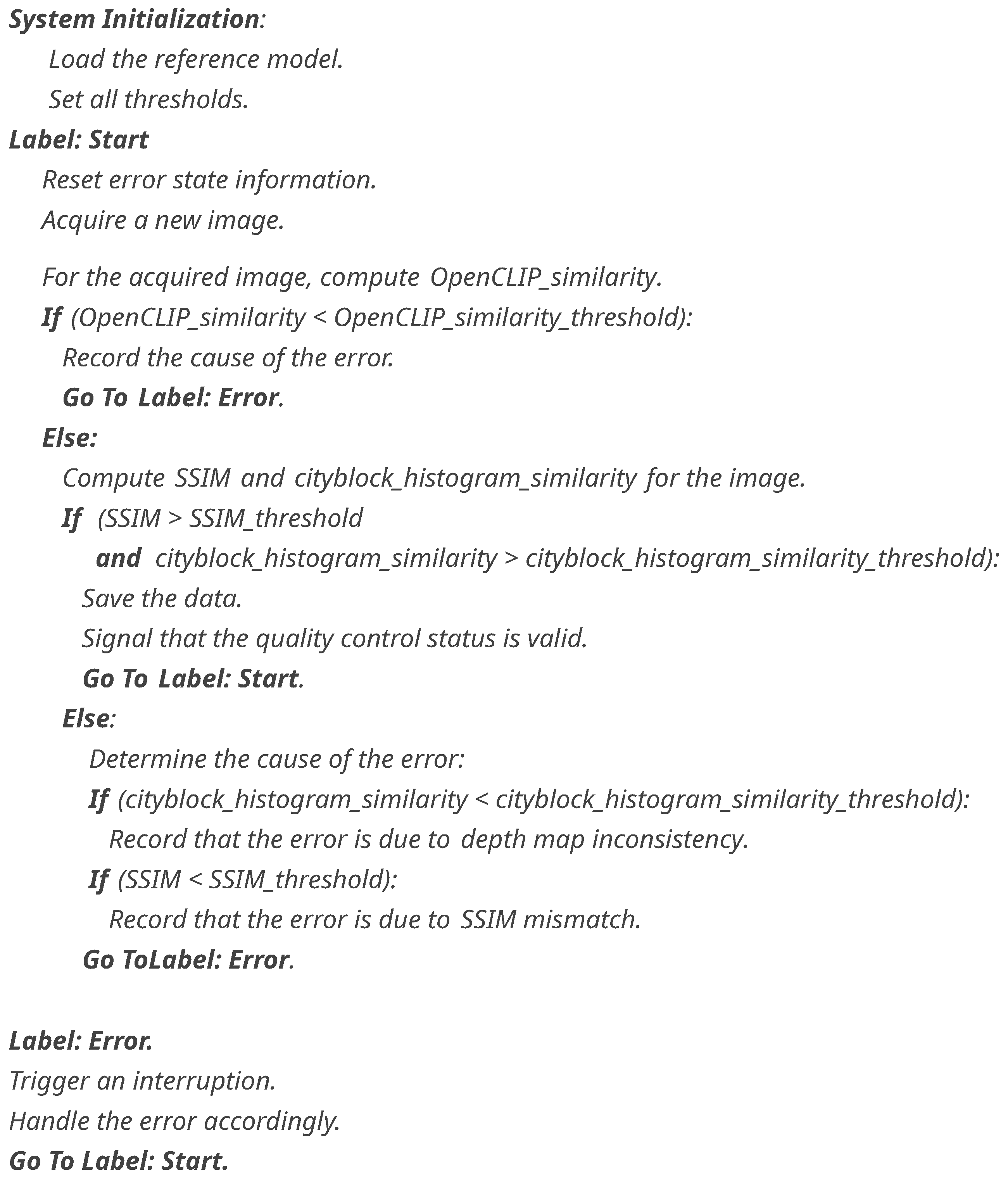
The above Sections present the fundamental components necessary for constructing the quality control algorithm (Figure 7). Its operation is described below in a simplified manner, focusing on a single measurement cycle. For clarity, the description excludes the statistical analysis of results variability over time. The draft of the algorithm with described flows and key decision points is shown in Figure 7.

4. Tests, Discussion and Future Work

The tests were conducted on a simplified test stand with manual sample feeding. Calculations were performed using the dedicated hardware platforms, with each metric computed independently. The experiments focused on evaluating the core components of the algorithm rather than a fully deployable system. The fixed decision thresholds were set for a specific environment (machine, configuration, lighting) based on observations of quality indicators derived from small image datasets. Alternative adaptive weighting and rule learning represent established and rapidly evolving approaches in the domains of metric fusion and visual inspection. Adaptive weighting techniques enhance the efficacy of image-based classification and defect detection by dynamically modulating the significance of diverse data sources or features—a well-supported principle by extensive research work in image processing and machine learning [34]. Conversely, rule learning is a pivotal component of visual inspection systems, enhancing their flexibility and capacity to adapt to changing manufacturing conditions. The practical deployment of these methodologies within small to medium-sized enterprises is frequently impeded by contextual constraints, including resource scarcity, time limitations, and the high variability inherent in the products being inspected [35].

Moreover, unlike CNN-based classifiers, which require extensive, well-annotated datasets and time-consuming training, the presented approach enables immediate deployment without hours-long model training. The planned future work will involve developing systematic procedures for threshold selection and performing sensitivity analyses to assess the impact of variations in thresholds.

For the NVIDIA Jetson Nano, the computation times for the considered similarity metrics are as follows:

• SSIM—0.012 s;
• Cityblock—0.025 s;
• OpenCLIP similarity—0.021 s.

For the Intel platform, the corresponding times were:

• SSIM—0.08 s;
• Cityblock—0.07 s;
• OpenCLIP similarity—0.12 s.

The impact of CUDA acceleration on the Jetson Nano platform is noticeable. The computation times are acceptable and are shorter than the time required to fill a mold.

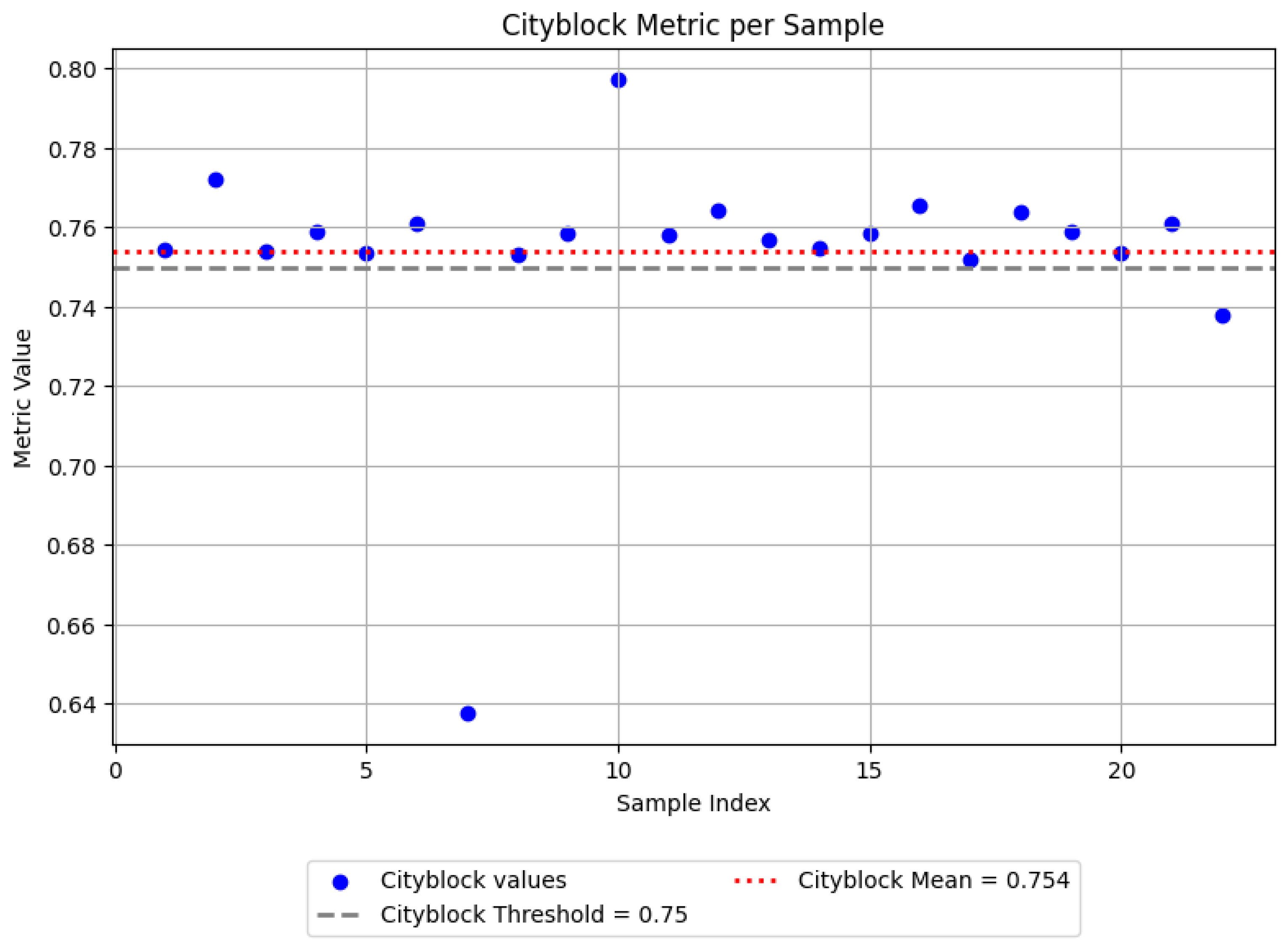
Based on the analysis of the distribution of similarity scores presented in the plots (Figure 8 and Figure 9), it can be observed that the mean values (

Table 1. Descriptive statistics for valid samples.

Metric	Mean	Std Dev	Min	Max	Range
OpenCLIP1	0.4559	0.1102	0.3422	0.7455	0.4033
OpenCLIP2	0.4871	0.0850	0.3456	0.6890	0.3434
SSIM	0.8931	0.1136	0.5477	0.9732	0.4255
Cityblock	0.7539	0.0281	0.6377	0.7972	0.1595

) for both SSIM and Cityblock metrics are aligned with the predefined thresholds. In certain applications, the use of average values could serve as a reasonable basis for estimating threshold levels, particularly in scenarios where empirical calibration is not feasible.

The experimental dataset comprises 31 samples, 8 of which were excluded from the statistical evaluation due to their manual preparation for illustrative purposes. For the actual performance evaluation and metric validation, a significantly larger dataset comprising 450 real-world images collected during production was used. This extended dataset enabled a more representative and statistically meaningful analysis, including the calculation of classification metrics such as Accuracy, Precision, Recall, and F1-score. The dataset of 450 images represents 3 months of production in a typical small bakery (20–30 molds/h × 8 h × 22 working days × 3 months). This is a realistic size for validation in this type of production environment, where defects occur sporadically.

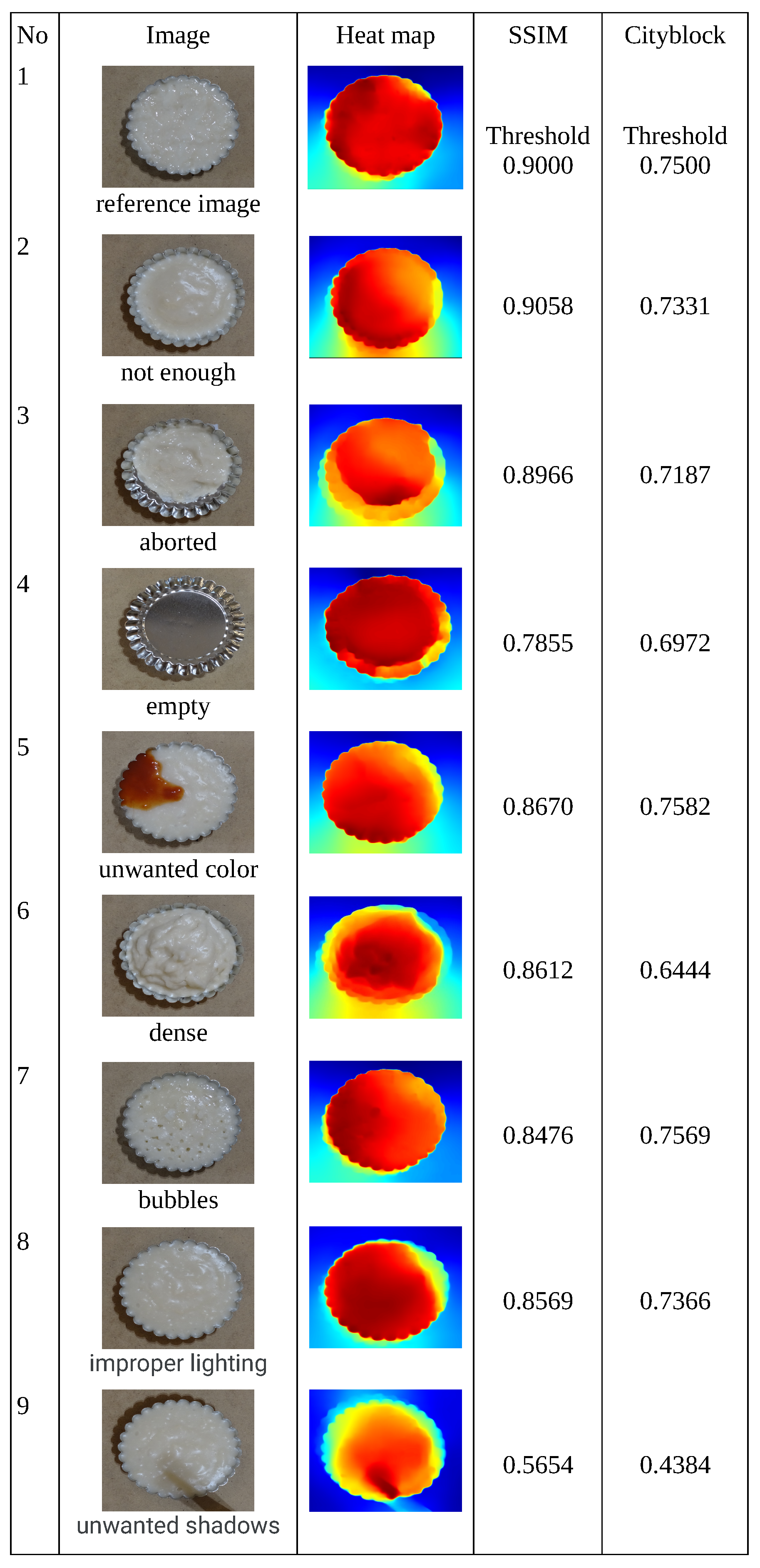
Figure 10 presents a collection of dough mold images, starting with a reference sample, followed by examples subject to various types of degradation. The first four images, from top to bottom, illustrate filling issues, ranging from a properly filled mold to an empty one. The remaining images depict typical observations after a pump problem, as illustrated in Figure 1.

Figure 11 and Figure 12 illustrate a metric designed to assess the semantic consistency of a scene based on natural language prompts. This metric is employed to detect visual artifacts that may compromise the reliability of other quality indicators. In the experiments, the similarity threshold for the overexposed image (example OpenCLIP1) was set at 0.7, while for the image with shadows (example OpenCLIP2), the threshold was set at 0.6. This metric reflects the semantic consistency of the scene based on natural language prompts and is used to detect visual artifacts that may affect the reliability of other quality indicators.

Among all metrics (Table 1), SSIM exhibits the highest standard deviation ($\sigma =0.1136$), indicating substantial variability across the samples. The SSIM is highly sensitive to visual differences between samples. In contrast, Cityblock shows the lowest standard deviation ($\sigma =0.0281$), reflecting high consistency and stability in its values.

The SSIM metric also demonstrates the widest range ($0.4255$), further confirming its sensitivity to subtle changes in image structure. On the other hand, Cityblock has the narrowest range ($0.1595$), which may make it a reliable reference metric for detecting more pronounced deviations.

• SSIM ranges from $0.5477$ to $0.9732$, with several samples falling below the commonly accepted threshold of $0.9$. This indicates that even among valid samples, SSIM may flag borderline cases.
• OpenCLIP1 values range from $0.3422$ to $0.7455$, with only one sample exceeding the threshold of $0.7$, confirming its effectiveness in identifying negative cases.
• Cityblock values are tightly clustered between $0.6377$ and $0.7972$, with most values hovering near the threshold of $0.75$.
• OpenCLIP1 and OpenCLIP2 demonstrate strong alignment with their respective thresholds, making them effective for distinguishing between valid and invalid samples.
• SSIM, while sensitive and informative, may produce false positives in borderline cases due to its high variability.
• Cityblock stands out as the most stable metric, suggesting its potential as a reference or supporting indicator in multi-metric evaluation systems.
• These findings support the idea that no single metric is sufficient for robust classification.

In future research, the integration of multiple evaluation metrics—through approaches such as weighted scoring systems or rule-based decision logic—may improve the robustness and reliability of the classification process while reducing the likelihood of misclassification.

One of the captured issues involves color distortion. In this case, the Cityblock assessment exceeds the acceptance threshold, suggesting correct mold filling. However, the SSIM value falls below the threshold, correctly indicating a defect. This sample should be rejected, similar to cases involving texture variations caused by air bubbles. For density-related changes, both metrics behave as expected. The last two cases were rejected due to the OpenCLIP similarity exceeding the predefined threshold, which acts as a safeguard against incorrect classification.

Classification methods are evaluated using various metrics that quantify their performance [36]. The most commonly used metrics are Precision, Recall, Accuracy, and F1-score [37]. These metrics are derived from the confusion matrix, which consists of the numbers of True Positives (TP), True Negatives (TN), False Positives (FP), and False Negatives (FN).

Precision measures the proportion of true positive predictions among all positive predictions.

$$\mathrm{Precision}={\displaystyle \frac{TP}{TP+FP}}$$

(1)

Recall (Sensitivity) measures the proportion of true positive predictions among all actual positive instances.

$$\mathrm{Recall}={\displaystyle \frac{TP}{TP+FN}}$$

(2)

Accuracy measures the proportion of correctly classified instances among all instances.

$$\mathrm{Accuracy}={\displaystyle \frac{TP+TN}{TP+TN+FP+FN}}$$

(3)

F1-score is the harmonic mean of Precision and Recall, providing a balance between the two.

$$\mathrm{F}1\text{-}\mathrm{score}=2·{\displaystyle \frac{\mathrm{Precision}·\mathrm{Recall}}{\mathrm{Precision}+\mathrm{Recall}}}$$

(4)

The results presented in

Table 2. Classification metrics (Accuracy, Precision, Recall, F1-score) for OpenCLIP-based filtering of negative image attributes (overexposure and shadows).

Prompt	Accuracy	Precision	Recall	F1-Score
“the scene is overexposed”	0.9667	0.9655	0.9912	0.9782
“shadows are present”	0.9412	0.7500	0.9882	0.8083

,

Table 3. Classification metrics (Precision, Recall, Accuracy, F1-score) for thresholded SSIM, Cityblock, and their combination on the full dataset with shadow and overexposure artifacts.

Metrics	Precision	Recall	Accuracy	F1-Score
SSIM	0.8866	0.9778	0.8417	0.9215
Cityblock	0.8598	0.9479	0.8908	0.9010
SSIM & Cityblock	0.9151	0.9604	0.8908	0.9372

and

Table 4. Classification metrics (Precision, Recall, Accuracy, F1-score) for thresholded SSIM, Cityblock, and their combination on the filtered dataset after OpenCLIP-based exclusion of shadow and overexposure artifacts.

Metrics	Precision	Recall	Accuracy	F1-Score
SSIM	0.8866	0.9885	0.8584	0.9348
Cityblock	0.8598	0.9583	0.9304	0.9064
SSIM & Cityblock	0.9151	0.9898	0.9464	0.9510

provide insight into the effectiveness of different filtering strategies applied to image datasets affected by shadows and over-lighting. Each element of the developed hybrid solution may be characterized by different properties. Therefore, they are complementary to each other and should be used together.

• OpenCLIP—Semantic Filter Function:
  OpenCLIP acts as a semantic filter that gates the acceptance of images before depth and similarity measures are applied. This filter operates as a pre-selection step, removing images affected by shadows and overexposure, thus preventing the propagation of errors to subsequent stages.
• MiDaS (Cityblock) and SSIM—complementary roles:
  SSIM is sensitive but variable; Cityblock is stable but less sensitive. The combined method improves detection effectiveness (Table 3 and Table 4). Cityblock, which is derived from MiDaS depth maps, contributes stability and geometric information; SSIM provides sensitivity to visual differences. Their combination achieves the best F1-scores, as shown in classification tables.
• Direct Impact on Robustness:
  Tables demonstrate the complementary roles of MiDaS (Cityblock) and OpenCLIP for robust classification by disabling similarity measurements on problematic images.

In Table 2, the OpenCLIP filtering criteria show high accuracy and recall for both shadowed and over-lighted images. Notably, the precision for shadow detection remains high ($0.9655$), indicating reliable identification of true positives. However, over-lighting detection exhibits a lower precision (0.7500), suggesting a higher rate of false positives despite excellent recall (0.9882).

Table 3 compares three methods—SSIM, Cityblock, and their combination—on the full dataset. The combined method (SSIM & Cityblock) achieves the highest precision ($0.9151$) and F1-score ($0.9372$), demonstrating the benefit of ensemble filtering. Interestingly, the accuracy of Cityblock and the combined method is identical ($0.8908$), but the combined method outperforms in precision and recall.

Table 4 presents the metrics after applying filtering. The SSIM & Cityblock method maintains its precision ($0.9151$) while improving both accuracy (to $0.9464$) and recall (to $0.9898$). This stability in precision across filtering stages suggests that the filtering process effectively reduces false negatives without introducing additional false positives.

Overall, the results indicate that combining SSIM & Cityblock metrics yields robust filtering performance, especially when applied to preselected datasets. The consistent precision values reinforce the reliability of the positive predictions, while improvements in recall and F1-score highlight enhanced detection capability post-filtering.

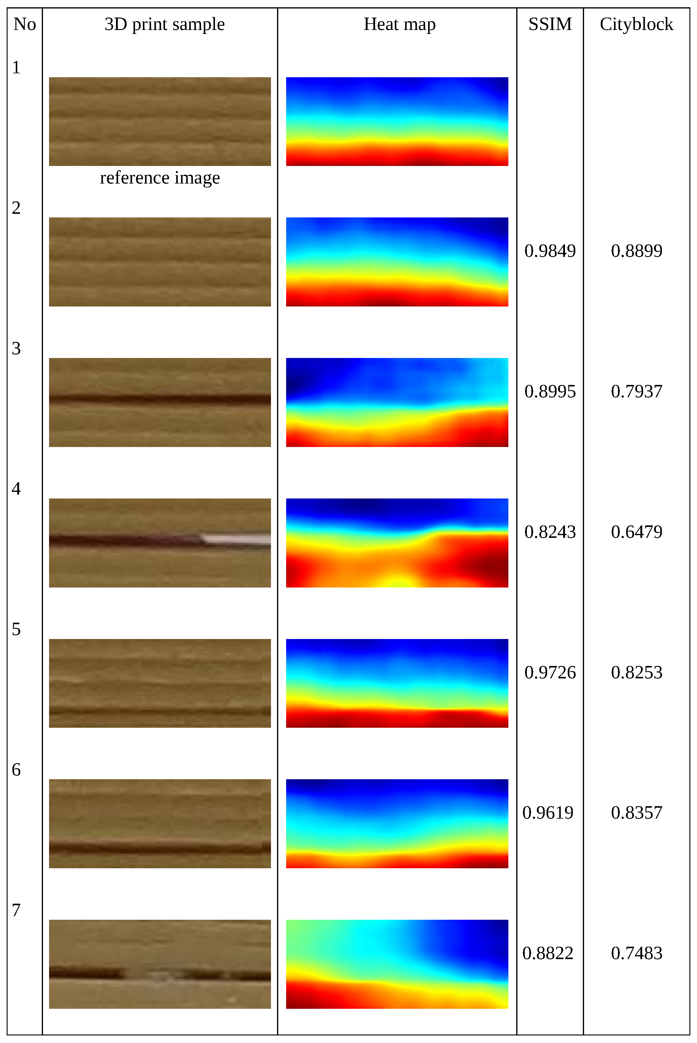
The reliability of the algorithm’s key components, verified using images of dough molds and the previously discussed example involving various tube placements, inspired the exploration of new application areas. In a visual context, the side-by-side arrangement of the tubes resembles the appearance of layers in 3D-printed objects. As illustrated in Figure 13, several samples produced by a 3D printer are presented, including both a correctly printed object and examples with visible defects, consistent with previous findings in real-time 3D printing control [38,39]. Samples from rows 1 and 2 represent successful prints that provide adequate structural strength.

The corresponding metric values could serve as threshold references, below which a 3D print should be considered defective. The remaining samples exhibit flaws that may disqualify the printed objects. The observed inversion in metric scores between samples 5 and 6, both of which exhibit lower-edge defects, may be attributed to differences in surface uniformity. The fact that SSIM is higher for sample 5, while Cityblock is higher for sample 6, may reflect variations in surface flatness above the defect. This highlights the sensitivity of the methods to specific geometric features and underscores the need for further investigation into their robustness. The interpretation of the results in this case can be more difficult than in the example with form filling. The increasing availability of 3D print sample databases, combined with subjective assessment of print quality, will support more accurate validation of the algorithm in future studies.

The future work may include selected benchmarking against new industrial image quality datasets [40].

5. Conclusions

This paper presented a hybrid visual quality control algorithm tailored for budget IIoT Edge devices. By combining SSIM, monocular depth estimation (MiDaS), and OpenCLIP-based semantic filtering, the system enables defect detection while maintaining low computational requirements. Preliminary experimental results confirm its applicability in both liquid mold filling and 3D printing scenarios. This approach aligns with the broader vision of Industry 5.0, where decentralized Edge Computing plays a central role [7]. This research addresses a significant gap in IIoT literature, which predominantly focuses on large-scale industrial deployments with substantial computational resources. Small and medium enterprises (SMEs) represent the majority share of businesses in the European Union food sector, yet existing IIoT solutions are often economically inaccessible to them. This pragmatic approach prioritizes immediate deployability and cost-effectiveness over algorithmic sophistication—a necessary compromise for democratizing IIoT adoption in resource-constrained environments. The scientific contribution of this work is multifaceted. It includes the development and validation of a novel hybrid algorithm, the definition of its conceptual structure, and the verification of its core components. The integration of complementary methods enhances reliability and adaptability, while the presented framework provides a solid foundation for future implementations and extensions.

This work lays the groundwork for further research, including adaptation to diverse industrial processes and integration into real-time Edge Computing environments.