Short-Term Wind Power Forecasting Based on ISFOA-SVM

Abstract

Short-term wind power prediction is critical for stable power system operation, but the non-stationarity and randomness of wind power output hinder prediction accuracy. To address this, this study proposes an improved superb fairy-wren optimization algorithm (ISFOA), which dynamically adjusts search step size via an adaptive learning factor to enhance global exploration and integrates a differential evolution strategy to optimize local search, improving convergence speed and optimization accuracy. Convergence analysis based on the Markov chain model verifies ISFOA’s stability. The ISFOA is combined with a Support Vector Machine (SVM) to construct the ISFOA-SVM model for short-term wind power prediction and is validated on real datasets from a southern China wind farm. Performance comparisons with four state-of-the-art models (SFOA-SVM, PSO-SVM, MFO-SVM, and GWO-SVM) show ISFOA-SVM achieves the best results across all metrics: MAE (0.3158), MBE (0.0126), RMSE (0.3304), and $R^2$ (0.9982). Compared to SFOA-SVM, it reduces RMSE by 67.08%, MBE by 54.68%, MAE by 1.10%, and increases $R^2$ by 0.34%. It outperforms PSO-SVM and MFO-SVM, which show intermediate results, and GWO-SVM, which exhibits the worst MAE, RMSE, and $R^2$ despite better MBE. These results confirm ISFOA-SVM’s effectiveness in improving short-term wind power prediction accuracy.

1. Introduction

The escalating global energy crisis and worsening environmental pollution have emerged as pressing challenges confronting modern societies. Wind energy, as a renewable energy source characterized by abundant reserves, low carbon emissions, and relatively low operational costs, has been widely recognized as a pivotal solution to address these intertwined issues [1]. However, the intrinsic variability and intermittency of wind resources lead to non-stationary and stochastic characteristics in wind power output, which significantly threaten the stability and reliability of contemporary power systems [2]. Against this backdrop, accurate short-term wind power forecasting has become indispensable for mitigating such uncertainties and facilitating the efficient integration of wind energy into the power grid. Specifically, it plays an irreplaceable role in optimizing power dispatch strategies, guiding rational grid planning, and enhancing overall energy utilization efficiency [3].

In recent years, methods that combine intelligent optimization algorithms with machine learning models have achieved significant progress in the field of wind power forecasting, emerging as an effective approach to overcoming the limitations of traditional methods [4]. For instance, the study [5] proposed an ICEEMDAN-LSTM-TCN-Bagging model, which integrates improved complete ensemble empirical mode decomposition with adaptive noise (ICEEMDAN), long short-term memory (LSTM) networks, temporal convolutional networks (TCNs), and Bagging-based ensemble learning. This hybrid framework effectively reduces sequence complexity while improving prediction accuracy and generalization capability. Similarly, the work [6] introduced an enhanced CNN-BiLSTM architecture for load forecasting in power systems under uncertainty; Wan Sicheng et al. proposed a composite modeling and prediction method for power load (CMPLF) that integrates short-term and medium-term forecasting modules to enhance prediction stability [7]. Furthermore, to address the uncertainties associated with multiple power sources and loads, the study [8] presented a two-stage multi-objective optimization framework for power supply–demand balance, achieving economically reliable dispatch strategies. In addition, particle swarm optimization (PSO) is frequently integrated with deep learning architectures, such as bidirectional long short-term memory (BiLSTM) networks and attention-based temporal convolutional networks (TCNs) [9], to enhance the robustness and adaptability of forecasting models.

Over the past decade, wind power forecasting has rapidly evolved from single-site point estimates to regional, multi-step, and real-time applications. Abad-Santjago et al. [10] fused the Weather Research and Forecasting model with the European Centre for Medium-Range Weather Forecasts Reanalysis v5 (ERA5) and Machine Learning (ML) into a hybrid framework. Mansoor et al. [11] proposed a Feature Fusion Networks–Temporal Convolution Network (FFN-TCN) that operated under lightweight hyper-parameter tuning. To address distribution shift and channel entanglement in the vanilla Transformer, Gao et al. [12] introduced the De-Stationary–De-Stationary Channel Transformer (DT-DSCTransformer) and obtained state-of-the-art accuracy on ultra-short-term horizons. Wang et al. [13] further combined WaveNet with a Multi-gate Mixture-of-Experts (MMoE) architecture, leveraging shared-private networks to suppress error accumulation in multi-step predictions. The coupling of optimizers and neural networks has also enhanced generalization capability. Zhao and Bai [14] embedded a Modified Sine Algorithm Adaptive Dung Beetle Optimizer (MSADBO) into a Long Short-Term Memory (LSTM) network. Khamari et al. [15] developed a hybrid Surface Normal Gabor Filter–Recalling Enhanced Recurrent Neural Network–Sand Cat Swarm Optimization (SNGF-RERNN-SCSO) pipeline. Regional forecasting and data completion are emerging as new research frontiers. Konstantinou and Hatziargyriou [16] employed Bayesian Feature Selection to partition and prune redundant sub-regions for three south-eastern European countries. Zhang et al. [17] constructed a Conditional Generative Adversarial Network–Convolutional Neural Network–Long Short-Term Memory (CGAN-CNN-LSTM) framework.

Support Vector Machines (SVMs) have been widely adopted due to their solid theoretical foundation in statistical learning theory and their ability to handle high-dimensional nonlinear problems [18]. Numerous studies have focused on improving SVM performance by optimizing its parameters using intelligent algorithms. For example, the study [19] proposed an SVM model based on an improved seagull optimization algorithm (ISOA), which incorporates tent map initialization, a dynamic cosine learning factor, and Gaussian mutation strategies to enhance convergence and search accuracy. Wang Li et al. applied an ant colony algorithm-optimized least squares support vector machine to short-term load forecasting, significantly improving prediction accuracy and reducing computational time [20].

Table 1. Several studies on wind power forecasting methods.

Cite	Method	Applicable Scenarios
[5]	ICEEMDAN-LSTM-TCN-Bagging	Short-term power load prediction
[6]	CNN-BiLSTM	Power load prediction
[7]	CMPLF	Power load prediction
[8]	TSMO	Power supply and demand balance
[19]	ISOA-SVM	Electric power load forecasting
[20]	ACA-LSSV	Load prediction
[10]	ERA5 and ML	Wind power forecasting
[11]	FFN-TCN	Wind power forecasting
[12]	DT-DSCTransformer	Ultra-short-term wind power forecasting
[13]	WaveNet	Multi-step wind power prediction
[14]	LSTM embedded with MSADBO	Ultra-short-term wind power forecasting
[15]	SNGF-RERNN-SCSO pipeline	Wind power forecasting
[16]	Bayesian Feature Selection	Regional wind power forecasting
[17]	CGAN-CNN-LSTM framework	Ultra-short-term wind power forecasting
[9]	TCN	Short-term power load forecasting

summarizes representative research methods and their applicable scenarios in the field of wind power and related load forecasting in recent years.

Existing literature exhibits a paucity of rigorous theoretical convergence guarantees for optimization algorithms deployed in wind-integrated power systems. Moreover, under pronounced wind-power fluctuations, these algorithms manifest limited convergence rates and impaired predictive accuracy [19]. The ISFOA-SVM model proposed in this study improves the SFOA algorithm by introducing an adaptive learning factor and a differential evolution strategy, enhancing global search and convergence speed, and solving the parameter sensitivity problem of traditional SVM. Experiments under different conditions verify its advantages in prediction accuracy and stability, providing a more reliable solution for wind power forecasting. The main contributions of this study can be summarized as follows:

1.

An improved version of the superb fairy-wren optimization algorithm (ISFOA) is proposed to optimize the hyperparameters of the SVM model. This enhancement significantly improves the algorithm’s convergence performance and global search ability.

2.

Based on the Markov chain model, the convergence analysis of ISFOA is presented.

3.

A hybrid forecasting model named ISFOA-SVM is constructed by integrating ISFOA with SVM, which effectively addresses the parameter sensitivity issue in traditional SVM and enhances prediction accuracy.

4.

The proposed ISFOA-SVM model is applied to short-term wind power forecasting, demonstrating superior performance in terms of prediction accuracy, stability, and generalization compared to existing benchmark models.

5.

Extensive experiments are conducted on real-world wind power datasets, and the results validate the effectiveness and robustness of the proposed method under different weather and operational conditions.

The remainder of this paper is organized as follows: Section 2 introduces the theoretical foundations of the SVM model. Section 3 presents a detailed description of the original SFOA and the proposed ISFOA algorithm. The global convergence analysis of ISFOA can be seen in Section 4. Section 5 outlines the construction and implementation of the ISFOA-SVM forecasting model, followed by experimental results and discussions. Finally, Section 6 concludes the paper with a summary of contributions and suggestions for future research.

2. Support Vector Machine

Support vector machines, as a powerful class of supervised machine learning algorithms, have been widely applied in both classification and regression tasks due to their strong generalization ability and global optimization characteristics. The core idea of SVM is to find an optimal regression plane that minimizes the prediction error while maintaining good generalization performance. Figure 1 provides a schematic illustration of its prediction process. In SVM modeling, each input sample $x_i$ in a low-dimensional space is first mapped into a higher-dimensional feature space through a nonlinear mapping function $\varphi \left(x\right)$. Subsequently, a linear regression function is constructed in this high-dimensional space, which can be expressed as follows [21]:

$$f\left(x\right)=\mathit{\omega }·\varphi \left(x\right)+bx\in {\mathbb{R}}^d,b\in \mathbb{R}$$

(1)

where $\mathit{\omega }$ denotes the weight vector, b represents the bias term, and $f\left(x\right)$ is the predicted output corresponding to the input vector x. Here, d indicates the dimensionality of the input space, and $\mathbb{R}$ denotes the real number field.

To transform the regression problem into a tractable optimization task, the structural risk minimization principle is adopted. Specifically, a tolerance parameter $\epsilon$ is introduced to define an insensitive loss zone, within which errors are not penalized. To account for samples outside this zone, two slack variables ${\xi }_i$ and ${\xi }_i^{*}$ are added to relax the constraints. The resulting optimization problem is formulated as [22]:

$$\underset{\mathit{\omega },b,\xi ,{\xi }^{*}}{min}{\displaystyle \frac{1}{2}}{\parallel \omega \parallel }^2+C\sum _{i=1}^n({\xi }_i+{\xi }_i^{*}),$$

(2)

Subject to the following constraints:

$$\left\{\begin{array}{c}{y}_i-\mathit{\omega }·x_i-b\le \epsilon +{\xi }_i,\hfill \\ \mathit{\omega }·x_i+b-y_i\le \epsilon +{\xi }_i^{*},\hfill \\ {\xi }_i\ge 0,{\xi }_i^{*}\ge 0,\hfill \end{array}\right.i=1,2,\cdots ,n,$$

(3)

where n is the total number of training samples, C is the regularization (penalty) parameter balancing model complexity and training error, and $\epsilon$ defines the width of the insensitive loss zone. Larger values of C impose stronger penalties on deviations beyond $\epsilon$, potentially leading to overfitting, whereas smaller values may result in underfitting due to reduced model capacity.

To solve this constrained optimization problem, the Lagrange multiplier method is employed. By constructing the Lagrangian function and applying the duality theorem, the original problem is transformed into a dual optimization problem involving the maximization of the following objective function [23]:

$$\begin{array}{c}max\left\{\begin{array}{c}-{\displaystyle \frac{1}{2}}{\displaystyle \sum _{i,j=1}^n}({\alpha }_i-{\alpha }_i^{*})({\alpha }_j-{\alpha }_j^{*})K(x_i,x_j)\hfill \\ +{\displaystyle \sum _{i=1}^n}({\alpha }_i-{\alpha }_i^{*})y_i-\epsilon {\displaystyle \sum _{i=1}^n}({\alpha }_i+{\alpha }_i^{*})\hfill \end{array}\right\}\hfill \\ \mathrm{s}.\mathrm{t}.{\displaystyle \sum _{i=1}^n}({\alpha }_i-{\alpha }_i^{*})=0{\alpha }_i,{\alpha }_i^{*}\in [0,C]\hfill \end{array}$$

(4)

where ${\alpha }_i,{\alpha }_i^{*}$ are the Lagrange multipliers associated with each constraint, and $K(x_i,x_j)=\varphi \left(x_i\right)·\varphi \left(x_j\right)$ denotes the kernel function used to compute the inner product in the high-dimensional space without explicitly performing the nonlinear mapping.

Based on the solution of the dual problem, the final regression function can be expressed as [24]:

$$f\left(x\right)=\sum _{i=1}^n({\alpha }_i-{\alpha }_i^{*})K(x_i,x)+b.$$

(5)

Among various kernel functions, the radial basis function (RBF) is often considered ideal for its wide convergence region and high resolution. Therefore, the RBF is selected as the kernel function in this study, defined as [25]:

$$K(x,x_j)=exp\left(-{\displaystyle \frac{\parallel x-x_j{\parallel }^2}{2{\delta }^2}}\right),$$

(6)

where $\delta$ controls the width of the RBF kernel.

Despite its effectiveness, the traditional implementation of SVM typically selects hyperparameters C and $\delta$ based on empirical knowledge or grid search. However, such methods may lead to suboptimal performance due to the diversity and complexity of real-world datasets. To overcome this limitation and enhance the robustness and accuracy of the model, an improved superb fairy-wren optimization algorithm is proposed in this work to automatically determine the optimal parameters for SVM.

3. Improved Superb Fairy-Wren Optimization Algorithm

This section presents a detailed description of both the original superb fairy-wren optimization algorithm (SFOA) and its improved variant. In addition, the flowchart of the proposed improved algorithm is provided to illustrate the overall optimization process.

3.1. Original Superb Fairy-Wren Optimization Algorithm

The superb fairy-wren optimization algorithm (SFOA) is a novel metaheuristic algorithm inspired by the social behavior patterns observed in superb fairy-wren populations [26]. The algorithm simulates three distinct behavioral phases: (1) the growth phase of young birds, (2) the feeding and breeding phase, and (3) the predator avoidance phase. These behaviors are mathematically modeled through Equations (8)–(10).

3.1.1. Initialization Strategy

Similar to most swarm intelligence algorithms, SFOA begins with a random initialization of the population within the search space:

$$X=\mathrm{rand}(0,1)\times (ub-lb)+lb,$$

(7)

where X denotes the global matrix representing the population of candidate solutions; $X_i$ corresponds to the i-th individual in the population; $x_{i,D}$ represents the value of the D-th dimension of the i-th individual; N is the total number of individuals; rand is a uniformly distributed random number in $[0,1]$; and $ub$, $lb$ denote the upper and lower bounds of the decision variables, respectively.

3.1.2. Phase I: Growth Phase of Young Birds

In this phase, the algorithm simulates the learning behavior of young birds acquiring experience from their environment. This mechanism enhances global exploration capability. The position update rule is defined as follows [26]:

$$X_{i,j}^{t+1}=X_{i,j}^t+lb+\mathrm{rand}\times (ub-lb),\mathrm{if}r>0.5,$$

(8)

where $X_{i,j}^{t+1}$ represents the updated position of the i-th bird in the j-th dimension after t iterations; $X_{i,j}^t$ is the current position; and r is a random threshold used to determine whether this phase is executed.

3.1.3. Phase II: Feeding and Breeding Phase

This phase mimics the feeding and cooperative breeding behavior among adult superb fairy-wrens. It emphasizes local exploitation around promising regions of the search space. The position update equation is given by [26]:

$$X_{i,j}^{t+1}=X_G+p\times (X_b-X_{i,j}^t),\mathrm{if}r<0.5\mathrm{and}s<20,$$

(9)

where $X_G=X_b\times C$, and $C=0.8$ is a constant coefficient. The danger threshold $s=20\times (r_1+r_2)$, where $r_1$ and $r_2$ are normally distributed random numbers. Here, $X_b$ denotes the current best solution found so far. The parameter p controls the step size and is defined as:

$$p=sin\left(2\times (ub-lb)+m\times (ub-lb)\right),$$

with $m=2\times {\displaystyle \frac{\mathrm{FEs}}{\mathrm{MaxFEs}}}$, where FEs represents the current number of function evaluations and MaxFEs is the maximum allowed number of evaluations.

3.1.4. Phase III: Predator Avoidance Phase

This phase simulates the escape behavior of superb fairy-wrens when detecting predators, which helps maintain population diversity and avoid premature convergence. The position update strategy incorporates a Levy flight mechanism [26]:

$$X_{i,j}^{t+1}=X_b+\mathrm{Levy}\left(d\right)\times k\times X_{i,j},\mathrm{if}r<0.5\mathrm{and}s>20,$$

(10)

where $\mathrm{Levy}\left(d\right)$ denotes the step size generated using the Levy flight distribution, which ensures long jumps for escaping local optima. The adaptive flight balance factor k is defined as:

$$k=0.2\times sin\left({\displaystyle \frac{\pi }{2}}-w\right),$$

and w is the call frequency value, calculated as:

$$w={\displaystyle \frac{\pi }{2}}\times {\displaystyle \frac{\mathrm{FEs}}{\mathrm{MaxFEs}}}.$$

These three phases work collaboratively to balance global exploration and local exploitation throughout the optimization process.

3.2. Improved Superb Fairy-Wren Optimization Algorithm

This subsection presents the key improvements introduced in the enhanced version of the superb fairy-wren optimization algorithm (ISFOA), including the adaptive learning factor and differential evolution strategy.

3.2.1. Adaptive Learning Factor

One limitation of the original SFOA algorithm lies in its relatively slow convergence speed and reduced accuracy during the growth phase of young birds, primarily due to their inexperience. To address this issue, an adaptive learning factor is introduced into the position update mechanism to dynamically adjust the search behavior based on the evolutionary state of individuals. Specifically, the relative change rate of the fitness value of each individual fairy-wren is defined as:

$$\nu ={\displaystyle \frac{\left|f\left(X_i^t\right)-f\left(X_b^t\right)\right|}{f\left(X_b^t\right)+\eta }},$$

(11)

where $i=1,2,\cdots ,N_p$, $X_i^t$ denotes the i-th individual at the t-th iteration, $f\left(X_i^t\right)$ is the corresponding fitness value, $f\left(X_b^t\right)$ represents the best fitness value in the current population, and $\eta$ is a small constant used to prevent division by zero. Based on this measure, the adaptive learning factor for the i-th fairy-wren at the t-th iteration is calculated using the logistic function:

$$c_i^t={\displaystyle \frac{1}{1+e^{-\nu }}}.$$

(12)

The updated position of each individual is then determined according to the following rules:

$$X_{i,j}^{t+1}=\{\begin{array}{}\mathrm{(13a)}& c_t{X}_{i,j}^t+lb+rand(ub-lb),r>0.5\mathrm{(13b)}& c_t{X}_G+p(X_b-X_{i,j}^t),r<0.5,s<20\mathrm{(13c)}& c_t{X}_b+Levy\left(d\right)k{X}_{i,j},r<0.5,s>20\end{array}$$

These equations incorporate the adaptive learning factor into all three behavioral phases of the original algorithm, thereby improving both convergence speed and solution accuracy.

3.2.2. Differential Evolution Strategy

To further enhance the global search capability and avoid premature convergence, a differential evolution (DE) strategy is integrated into the improved algorithm. In particular, the DE/best/1 mutation strategy with a dynamic scaling factor is employed to maintain population diversity and escape local optima [27]. The mutation vector for the i-th individual at the t-th iteration is generated as follows:

$$H_i^t=X_{\mathrm{best}}^t+F_i^t·(X_{p1}^t-X_{p2}^t),$$

(14)

where $H_i^t$ is the mutant vector, $p_1,p_2\in \{1,2,\cdots ,N_p\}$ are randomly selected indices such that $p_1\ne p_2$, and $F_i^t$ is the dynamic scaling factor computed as:

$$F_i^t=F_{\mathrm{str}}+(F_{\mathrm{end}}-F_{\mathrm{str}})·{\displaystyle \frac{f\left(X_i^t\right)-f\left(X_b^t\right)}{f\left(X_w^t\right)-f\left(X_b^t\right)}},$$

(15)

with $F_{\mathrm{str}}=0.4$, $F_{\mathrm{end}}=0.9$, and $f\left(X_w^t\right)$ representing the worst fitness value in the current population. Subsequently, a binomial crossover operation is applied to generate the trial vector $V_{ij}^t=(V_{i1}^t,V_{i2}^t,\cdots ,V_{id}^t)$ as follows:

$$V_{ij}^t=\left\{\begin{array}{cc}{H}_{ij}^t,\hfill & \mathrm{if}j=j_0\mathrm{or}\mathrm{rand}(0,1)\le Cr\hfill \\ X_{ij}^t,\hfill & \mathrm{otherwise}\hfill \end{array}\right.$$

(16)

where $j_0\in \{1,2,\cdots ,d\}$ is a randomly chosen index ensuring at least one dimension is inherited from the mutant vector, and $Cr\in [0,1]$ is the crossover probability.

Finally, the selection process is carried out by comparing the fitness values of the trial and original vectors:

$$X_i^{t+1}=\left\{\begin{array}{cc}{V}_i^t,\hfill & \mathrm{if}f\left(V_i^t\right)<f\left(X_i^t\right)\hfill \\ X_i^t,\hfill & \mathrm{otherwise}\hfill \end{array}\right.$$

(17)

This integration of DE significantly improves the exploration ability of the algorithm while maintaining its exploitation performance.

3.2.3. Flowchart of the Improved Algorithm

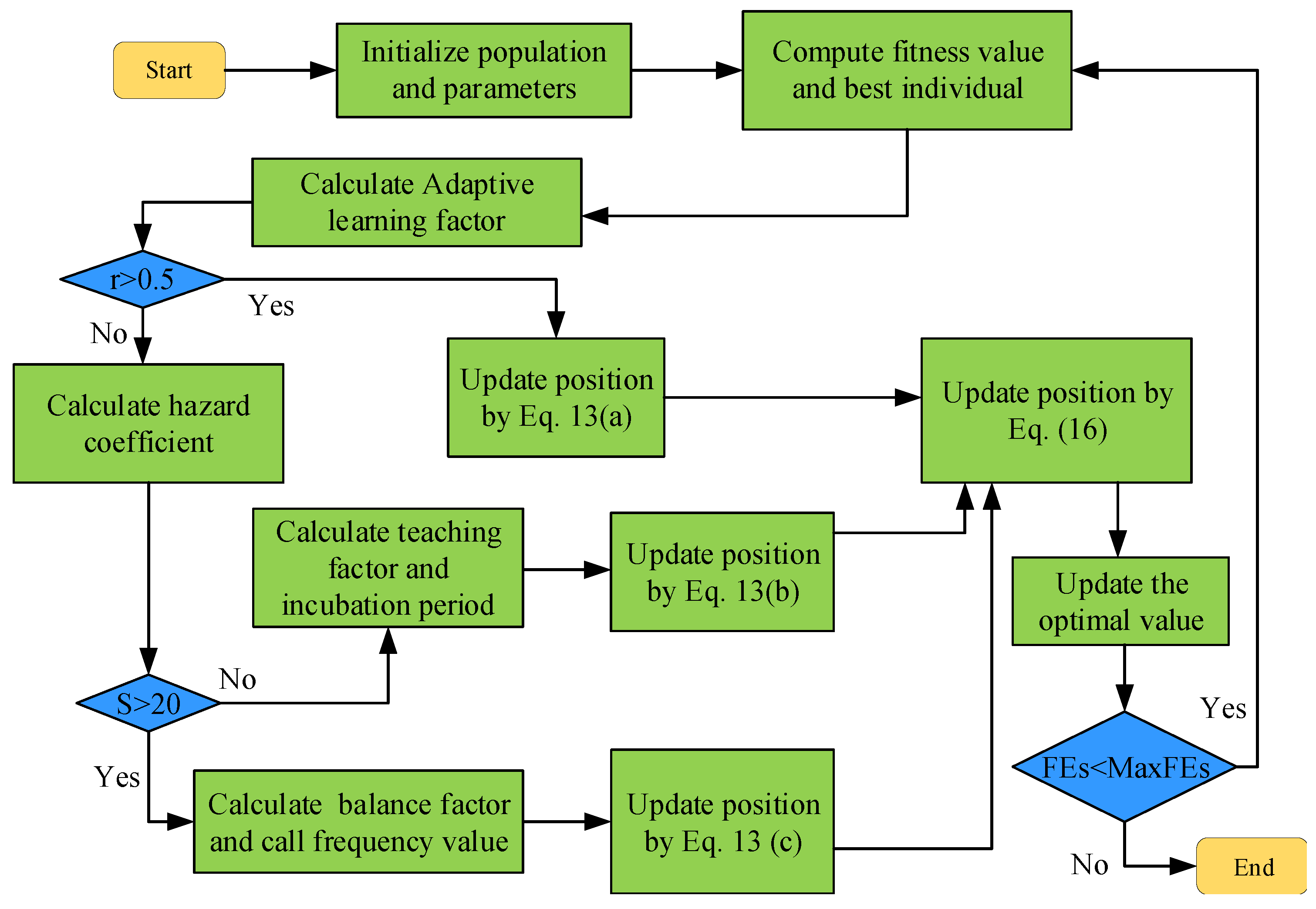
The overall framework of the ISFOA algorithm can be summarized as follows:

• Parameter Initialization: Set the maximum number of iterations (MaxFEs), problem dimension (d), population size ($N_p$), and the bounds of decision variables ($lb$, $ub$).
• Fitness Evaluation of Initial Population: Evaluate the fitness values of all individuals in the initial population and identify the best-performing solution.
• Position Update (Growth Phase of Young Birds):

  –

  If $r>0.5$, update positions using Equation (13a).

• Danger Threshold Assessment and Response:

  –

  Calculate the danger threshold s.

  –

  If $s<R$ (safe environment), perform breeding and feeding updates using Equation (13b).

  –

  Otherwise (dangerous environment), execute predator avoidance updates using Equation (13c).

• Differential Evolution Strategy Application: Apply the DE mutation and crossover operations described above to each individual.
• Fitness Re-evaluation: Recalculate the fitness values of the updated population and update the best solution.
• Termination Check: If the stopping criterion (e.g., reaching MaxFEs) is satisfied, terminate the algorithm and return the best solution found so far.

The complete flowchart of the ISFOA model is illustrated in Figure 2, providing a visual representation of the algorithm’s execution steps.

3.3. Performance Evaluation of ISFOA on CEC2022

In the field of intelligent optimization algorithm research, accurately evaluating the optimization performance of algorithms plays a crucial role in algorithm development and comparison. The CEC2022 benchmark test suite, characterized by its diverse function types and strict boundary constraints, has become a widely accepted standard for assessing the global search capabilities of optimization algorithms. This study aims to comprehensively evaluate the optimization performance of an improved variant of the Social Emotional Optimization Algorithm (ISFOA) using the CEC2022 test suite. Furthermore, the ISFOA is compared with five established metaheuristic algorithms: the original superb fairy-wren optimization algorithm (SFOA), Enzyme Action Optimizer (EAO) [28], Sine Cosine Algorithm (SCA) [29], Crayfish Optimization Algorithm (COA) [30], and Particle Swarm Optimization (PSO) [31].

The CEC2022 test suite comprises 12 single-objective benchmark functions, each defined within specified boundary constraints and exhibiting a wide range of functional characteristics. Among these, the unimodal function F1 is used to assess the local exploitation capability of the algorithms, requiring them to converge rapidly to the unique global optimum. Functions F2–F5 are multimodal, containing multiple local optima, and are used to evaluate the exploration ability of algorithms in escaping from suboptimal solutions. Hybrid functions (F6–F8) and composite functions (F9–F12) simulate complex real-world optimization problems by integrating various function properties, thereby imposing higher demands on the balance between exploration and exploitation.

All experiments were conducted in a controlled environment using a computer equipped with an Intel Core i5-12500 processor (3.00 GHz) and 16 GB of RAM, running the Windows 11 operating system. MATLAB R2022b was used as the programming and simulation platform for all algorithm implementations.

To ensure fairness in the comparison, all selected algorithms were executed using their default parameter settings. Each test function was independently evaluated 30 times to mitigate the influence of stochastic variations. The performance of each algorithm was assessed using two statistical measures: the mean best fitness value obtained across runs, which reflects the average convergence accuracy, and the standard deviation, which indicates the consistency and stability of the algorithm’s performance.

The performance of ISFOA was evaluated using the CEC2022 test functions, and it consistently outperformed or matched five mature metaheuristic algorithms in terms of convergence accuracy and stability. From

Table 2. Statistical results of ISFOA and five other comparative algorithms on the CEC2022 in 20 dimensions.

F*	Name	ISFOA	SFOA	COA	EAO	PSO	SCA
F1	Std	1.06 $\times {10}^3$	1.80 $\times {10}^6$	1.81 $\times {10}^4$	1.47 $\times {10}^4$	1.01 $\times {10}^4$	9.14 $\times {10}^3$
	Mean	1.43 $\times {10}^3$	1.09 $\times {10}^6$	6.35 $\times {10}^4$	3.44 $\times {10}^4$	2.93 $\times {10}^4$	2.95 $\times {10}^4$
F2	Std	2.59 $\times {10}^1$	2.92 $\times {10}^3$	5.75 $\times {10}^1$	6.47 $\times {10}^1$	2.82 $\times {10}^1$	1.62 $\times {10}^2$
	Mean	4.60 $\times {10}^2$	7.50 $\times {10}^3$	5.73 $\times {10}^2$	5.67 $\times {10}^2$	4.71 $\times {10}^2$	1.00 $\times {10}^3$
F3	Std	3.32 $\times {10}^0$	1.80 $\times {10}^1$	1.37 $\times {10}^1$	9.59 $\times {10}^0$	8.53 $\times {10}^0$	5.62 $\times {10}^0$
	Mean	6.04 $\times {10}^2$	7.11 $\times {10}^2$	6.46 $\times {10}^2$	6.81 $\times {10}^2$	6.16 $\times {10}^2$	6.55 $\times {10}^2$
F4	Std	3.27 $\times {10}^1$	3.94 $\times {10}^1$	1.28 $\times {10}^1$	1.55 $\times {10}^1$	2.10 $\times {10}^1$	1.89 $\times {10}^1$
	Mean	8.80 $\times {10}^2$	1.09 $\times {10}^3$	8.98 $\times {10}^2$	9.73 $\times {10}^2$	8.74 $\times {10}^2$	9.68 $\times {10}^2$
F5	Std	7.18 $\times {10}^1$	3.75 $\times {10}^3$	4.18 $\times {10}^2$	7.72 $\times {10}^2$	1.43 $\times {10}^2$	5.50 $\times {10}^2$
	Mean	9.76 $\times {10}^2$	1.32 $\times {10}^4$	3.20 $\times {10}^3$	2.95 $\times {10}^3$	1.05 $\times {10}^3$	3.10 $\times {10}^3$
F6	Std	3.36 $\times {10}^3$	3.59 $\times {10}^9$	2.57 $\times {10}^4$	4.45 $\times {10}^5$	1.40 $\times {10}^4$	1.73 $\times {10}^8$
	Mean	5.25 $\times {10}^3$	5.53 $\times {10}^9$	2.69 $\times {10}^4$	9.59 $\times {10}^5$	1.78 $\times {10}^4$	2.47 $\times {10}^8$
F7	Std	3.09 $\times {10}^1$	9.96 $\times {10}^1$	1.19 $\times {10}^2$	3.49 $\times {10}^1$	5.31 $\times {10}^1$	2.56 $\times {10}^1$
	Mean	2.08 $\times {10}^3$	2.48 $\times {10}^3$	2.19 $\times {10}^3$	2.24 $\times {10}^3$	2.13 $\times {10}^3$	2.21 $\times {10}^3$
F8	Std	3.30 $\times {10}^0$	1.07 $\times {10}^4$	5.99 $\times {10}^1$	6.20 $\times {10}^1$	8.06 $\times {10}^1$	5.69 $\times {10}^1$
	Mean	2.23 $\times {10}^3$	7.98 $\times {10}^3$	2.29 $\times {10}^3$	2.29 $\times {10}^3$	2.29 $\times {10}^3$	2.31 $\times {10}^3$
F9	Std	2.27 $\times {10}^{-1}$	4.31 $\times {10}^2$	3.43 $\times {10}^1$	3.35 $\times {10}^1$	3.87 $\times {10}^1$	4.73 $\times {10}^1$
	Mean	2.48 $\times {10}^3$	3.77 $\times {10}^3$	2.51 $\times {10}^3$	2.53 $\times {10}^3$	2.52 $\times {10}^3$	2.68 $\times {10}^3$
F10	Std	9.66 $\times {10}^2$	1.42 $\times {10}^3$	1.58 $\times {10}^3$	1.51 $\times {10}^3$	7.04 $\times {10}^2$	1.62 $\times {10}^3$
	Mean	2.81 $\times {10}^3$	7.49 $\times {10}^3$	5.29 $\times {10}^3$	2.99 $\times {10}^3$	3.40 $\times {10}^3$	3.33 $\times {10}^3$
F11	Std	1.63 $\times {10}^2$	5.10 $\times {10}^4$	1.07 $\times {10}^3$	1.02 $\times {10}^3$	1.21 $\times {10}^2$	1.48 $\times {10}^3$
	Mean	3.05 $\times {10}^3$	1.55 $\times {10}^5$	4.48 $\times {10}^3$	5.02 $\times {10}^3$	3.27 $\times {10}^3$	9.26 $\times {10}^3$
F12	Std	1.90 $\times {10}^1$	1.68 $\times {10}^2$	4.67 $\times {10}^1$	1.14 $\times {10}^2$	3.13 $\times {10}^1$	6.84 $\times {10}^1$
	Mean	2.98 $\times {10}^3$	3.76 $\times {10}^3$	3.01 $\times {10}^3$	3.11 $\times {10}^3$	2.99 $\times {10}^3$	3.15 $\times {10}^3$

The underlined numbers represent the best result in each row.

, it can be seen that ISFOA achieved the best average performance for 10 out of the 12 functions, including F1–F3, F5–F10, and F12. Specifically, for the unimodal function F1, ISFOA exhibited an average value of $1.43\times {10}^3$ and a standard deviation of $1.06\times {10}^3$, both of which were significantly better than those of SFOA, COA, EAO, PSO, and SCA. The low standard deviation indicates that ISFOA maintains high consistency and exhibits strong convergence stability across multiple runs. This outstanding performance is primarily attributed to the introduction of adaptive learning factors in ISFOA. Unlike the fixed update rules in SFOA, the adaptive learning factor dynamically adjusts the weights of individual experience and global guidance based on changes in fitness.

For the multimodal function F2, ISFOA achieved an average value of $4.60\times {10}^2$ and a standard deviation of $2.59\times {10}^1$, significantly outperforming SCA. For F5, the mean and standard deviation of ISFOA were much lower than those of SFOA. This indicates that ISFOA has a stronger ability to escape from local optima and maintain population diversity during the search process. This behavior is largely attributed to the integration of differential evolution (DE) strategies. The DE strategy enhances the exploration ability of the population by introducing new candidate solutions through mutation and crossover operations.

Despite the increased complexity of the mixed (F6–F8) and composite functions (F9–F12), ISFOA still maintained competitive performance. For instance, on F6, ISFOA achieved an average value of $5.25\times {10}^3$ and a standard deviation of $3.36\times {10}^3$, significantly outperforming SFOA and COA. At F10, ISFOA exhibited the best mean value ($2.81\times {10}^3$) and a relatively low standard deviation, surpassing PSO and SCA. These results highlight the robustness of ISFOA in handling high-dimensional, real-world-like optimization tasks. The combination of adaptive learning factors and differential evolution mechanisms enables ISFOA to dynamically adjust its search behavior based on problem characteristics, maintain population diversity while accelerating convergence, and effectively balance exploration and exploitation over time.

It should be noted that ISFOA still has some shortcomings in certain test functions. For example, in the F4 function, the standard deviation of ISFOA was $3.27\times {10}^1$ and the average value was $8.80\times {10}^2$, neither of which reached the optimal value. The standard deviation was significantly higher than that of COA ($1.28\times {10}^1$), and the average value was slightly higher than that of PSO ($8.74\times {10}^2$), indicating that its convergence accuracy and stability on this function were slightly inferior to some comparison algorithms. In the F7 function, the standard deviation of ISFOA was $3.09\times {10}^1$, while that of SCA was as low as $2.56\times {10}^1$, indicating that ISFOA’s stability performance in this function was inferior to that of SCA. This may be related to the parameter adjustment efficiency of ISFOA’s adaptive mechanism under specific function structures, reflecting the limitations of the algorithm in handling certain special forms of search spaces.

In summary, the experimental results based on the CEC2022 benchmark suite demonstrate that ISFOA outperforms existing algorithms in terms of convergence accuracy, search stability, and robustness. The integration of adaptive learning factors and differential evolution mechanisms significantly enhances the algorithm’s navigation ability in complex search spaces, helps avoid local optima, and effectively converges to the optimal solution.

Table 3. Results of Wilcoxon test for ISFOA against five comparative algorithms on the CEC2022.

F*	vs. SFOA	vs. COA	vs. EAO	vs. PSO	vs. SCA
F1	7.22 $\times {10}^{-64}$	5.86 $\times {10}^{-30}$	1.53 $\times {10}^{-53}$	2.55 $\times {10}^{-8}$	3.41 $\times {10}^{-1}$
F2	7.80 $\times {10}^{-65}$	5.51 $\times {10}^{-1}$	1.32 $\times {10}^{-34}$	2.29 $\times {10}^{-47}$	1.70 $\times {10}^{-40}$
F3	4.69 $\times {10}^{-65}$	1.91 $\times {10}^{-43}$	8.42 $\times {10}^{-52}$	7.76 $\times {10}^{-60}$	1.01 $\times {10}^{-9}$
F4	4.45 $\times {10}^{-65}$	5.69 $\times {10}^{-52}$	1.88 $\times {10}^{-39}$	2.22 $\times {10}^{-47}$	2.78 $\times {10}^{-8}$
F5	2.78 $\times {10}^{-66}$	1.97 $\times {10}^{-12}$	2.09 $\times {10}^{-35}$	6.92 $\times {10}^{-56}$	2.31 $\times {10}^{-10}$
F6	1.15 $\times {10}^{-64}$	3.02 $\times {10}^{-16}$	7.52 $\times {10}^{-39}$	8.06 $\times {10}^{-32}$	1.23 $\times {10}^{-43}$
F7	9.91 $\times {10}^{-65}$	2.12 $\times {10}^{-15}$	8.53 $\times {10}^{-48}$	2.83 $\times {10}^{-52}$	6.73 $\times {10}^{-3}$
F8	1.13 $\times {10}^{-67}$	1.34 $\times {10}^{-3}$	1.64 $\times {10}^{-42}$	4.61 $\times {10}^{-10}$	4.41 $\times {10}^{-19}$
F9	1.63 $\times {10}^{-63}$	8.92 $\times {10}^{-10}$	1.99 $\times {10}^{-41}$	1.47 $\times {10}^{-35}$	8.41 $\times {10}^{-28}$
F10	4.28 $\times {10}^{-64}$	8.28 $\times {10}^{-42}$	5.53 $\times {10}^{-7}$	1.83 $\times {10}^{-8}$	9.77 $\times {10}^{-4}$
F11	6.40 $\times {10}^{-64}$	1.08 $\times {10}^{-16}$	2.20 $\times {10}^{-27}$	2.54 $\times {10}^{-22}$	2.60 $\times {10}^{-53}$
F12	2.63 $\times {10}^{-62}$	1.03 $\times {10}^{-32}$	1.69 $\times {10}^{-42}$	1.96 $\times {10}^{-55}$	3.65 $\times {10}^{-8}$

presents the results of the Wilcoxon signed-rank test for the ISFOA algorithm against five comparative algorithms on the CEC2022 test set, with a significance level set at 0.05. The values in the table represent p-values, where underlined p-values indicate no significant difference in the corresponding comparison group (i.e., the p-value is greater than or equal to 0.05). The test results show that for most functions, such as F1–F6 and F8–F12, the p-values between ISFOA and each comparative algorithm are far less than 0.05. Only in function F1 is the p-value between ISFOA and SCA greater than or equal to 0.05, indicating no significant difference between the two. In function F2, the p-value between ISFOA and COA is also greater than or equal to 0.05, showing no significant difference in performance. Additionally, in function F7, the p-value between ISFOA and SCA is 6.73 $\times {10}^{-3}$, which is close to the critical value of the significance level. Overall, there are statistically significant differences in performance between ISFOA and the other comparative algorithms, namely SFOA, COA, EAO, and PSO.

Figure 3 shows the convergence curves of five competing algorithms on 12 different problems. For the unimodal function F1, the ISFOA algorithm exhibits the most outstanding performance. It benefits from the effective adjustment of the search-step size by the adaptive learning factor. Meanwhile, the differential evolution strategy optimizes the local search. Therefore, ISFOA has no tendency to fall into local optima. For the multimodal functions F2–F5, PSO and ISFOA are evenly matched in terms of convergence accuracy and speed. The performance of the remaining algorithms is in the middle. SFOA and SCA have poor convergence speed and accuracy. This indicates that the improvement strategies of ISFOA, namely the adaptive learning factor and the differential evolution strategy, have played a role. However, for F4, due to the characteristics of the problem, the convergence speed of ISFOA is weaker than that of PSO and COA. For the hybrid functions F6–F8, since F6 is a complex problem, the performance of each algorithm varies significantly. The adaptive learning factor of ISFOA gives it more advantages in global search. Although the final accuracy of two algorithms is comparable, due to the complexity of the F6 problem, the effect of its differential evolution strategy on speed-up is relatively limited, resulting in ISFOA being slightly inferior in speed. For F7 and F8, the differences between different algorithms are not obvious. In the case of composite functions, for F10, the performance of ISFOA is only better than that of SFOA. Compared with the other four algorithms, it is at a disadvantage and ranks second-last. EAO has the best convergence speed and accuracy. For F9, F11, and F12, due to the complexity of the problems, except for SFOA, ISFOA and the other four algorithms perform equally well. Overall, it is shown that ISFOA has obvious advantages in some problems, has bright spots in multimodal, hybrid, and some composite-function problems, but there is still room for improvement in some complex composite-function problems.

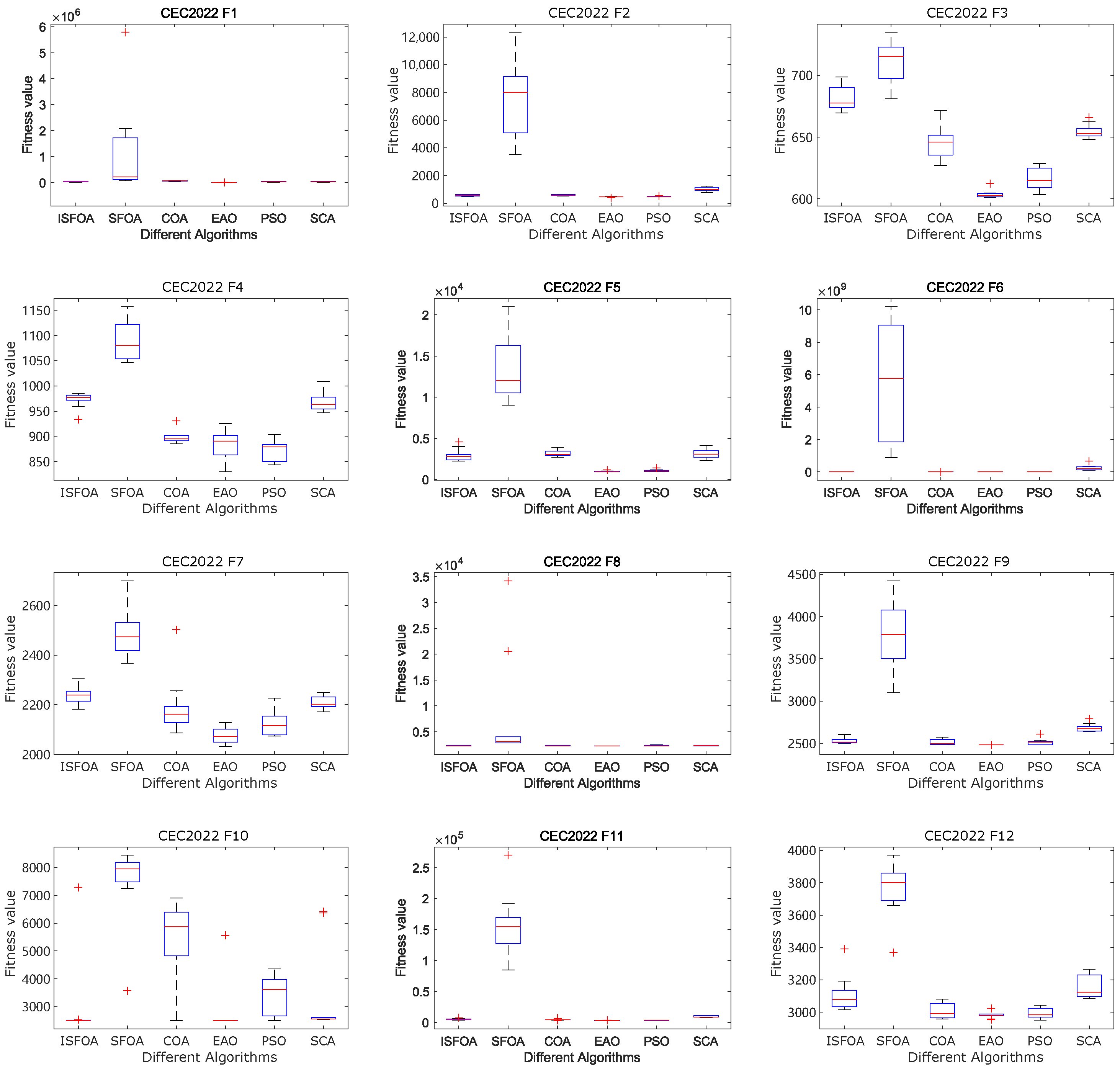
Box plots are commonly used to describe the dispersion of data. Their main advantage is that they are not affected by outliers. They can visually show the median, quartiles, range, and overall distribution trend of the data. Therefore, they are important tools for evaluating the performance and stability of optimization algorithms. Figure 4 presents box plots for 12 functions from CEC2020. These plots illustrate the distribution of results from 30 independent runs of each algorithm. For function, F3, ISFOA performs worse than the other four algorithms. This is due to the iterative update mechanism and parameter self-adaptive adjustment strategy used in ISFOA. These features make it difficult for ISFOA to consistently converge toward the global optimal solution in 30 runs. As shown in the box plot, this is reflected by a higher median and a wider spread, indicating poorer performance. For functions F4 and F7, COA, EAO, and PSO perform best. ISFOA and SCA are in the second tier. F4 and F7 are moderately complex continuous optimization problems. These problems require high algorithm stability. Although ISFOA and SCA lack precision in local search, their overall optimization mechanisms still provide a certain level of competitiveness. For function F10, which is a multimodal function, ISFOA performs the best. EAO and SCA are close behind. However, PSO and COA perform poorly on this function. Overall, the results indicate that ISFOA has strong competitive advantages.

4. Global Convergence Analysis of ISFO

4.1. Stochastic Process Modeling of the Algorithm

Modeling the iterative optimization of ISFOA as a state-transition stochastic process is fundamental for analyzing the algorithm’s convergence. Each update of ISFOA is determined by the current population state and random variables, and this “memorylessness” can be rigorously modeled as a Markov chain.

Definition 1

(Discrete-Time Stochastic Process). The population sequence ${\left\{X^t\right\}}_{t=0}^{\infty }$ in ISFOA can be regarded as a stochastic process defined on the probability space $(\Omega ,\mathcal{F},P)$, where $X^t=\{x_1^t,x_2^t,\dots ,x_N^t\}$ represents the population at the t-th generation. The state transition function $\mathcal{T}$ of each individual $x_i^t\in R^d$ includes the three-stage behaviors (growth, reproduction, predator avoidance), adaptive learning factors, and DE strategy. The population sequence of $t+1$-th generation can be written as

$$X^{t+1}=\mathcal{T}(X^t,{\xi }^t),{\xi }^t\sim \mathit{iid},$$

where ${\xi }^t$ means the sequence of random variables. $iid$ stands for independent and identically distributed.

Theorem 1

(Markov Property). The stochastic process ${\left\{X^t\right\}}_{t=0}^{\infty }$ generated by ISFOA is a time-homogeneous Markov chain. For any $t\ge 0$ and state sequences $x^0,x^1,\dots ,x^{t+1}\in {\Omega }^N$,

$$\begin{array}{c}P(X^{t+1}=x^{t+1}|X^t=x^t,\dots ,X^0=x^0)\hfill \\ =P(X^{t+1}=x^{t+1}|X^t=x^t).\hfill \end{array}$$

(18)

Proof. 

The state update rule of ISFOA depends only on the current population state $X^t$, the current best solution $X_b^t$, and random numbers. For any time t, the probability distribution of the next state $X^{t+1}$ is determined solely by $X^t$, regardless of $X^0,X^1,\dots ,X^{t-1}$. Therefore, the process satisfies the Markov property.

$$P\left(X^{t+1}\right|X^t,X^{t-1},\dots ,X^0)=P\left(X^{t+1}\right|X^t).$$

Furthermore, since the random number generation mechanism is time-invariant, the process is a time-homogeneous Markov chain. □

4.2. Definition of Absorbing State

Let the set of global optimal solutions be $Z^{*}=\{x\in \Omega |f\left(x\right)=f^{*}\}$, where $f^{*}={min}_{x\in \Omega }f\left(x\right)$. If the state $X^t$ contains a solution in $Z^{*}$ (i.e., there exists $x\in X^t$ such that $f\left(x\right)=f^{*}$), then $X^t$ is called an absorbing state. As the selection mechanism favors the preservation of optimal solutions, once the algorithm enters an absorbing state, the optimal solutions will remain preserved in all subsequent states. Therefore,

$$P(X^{t+1}\in Z^{*}|X^t\in Z^{*})=1.$$

(19)

4.3. Positive Transition Probability

Lemma 1.

For any non-absorbing state $X^t\notin Z^{*}$, there exists a positive probability $\delta >0$ such that the algorithm transitions to an absorbing state within finite steps. Therefore,

$$P(X^{t+1}\in Z^{*}|X^t\notin Z^{*})\ge \delta .$$

(20)

Proof. 

This paper presents the proof of positive transition probabilities for three strategies.

1.

Adaptive Learning Factor

The relative fitness difference is ${\nu }_i^t={\displaystyle \frac{|f\left(x_i^t\right)-f\left(X_b^t\right)|}{f\left(X_b^t\right)+ϵ}}$. The adaptive factor is $c_i^t={\displaystyle \frac{1}{1+e^{-{\nu }_i^t}}}$. For non-optimal individuals ($x_i^t\ne x_b^t$), the adaptive learning factor $c_i^t$ undergoes dynamic adjustment in accordance with variations in the fitness difference between $f\left(x_i^t\right)$ and the current optimal solution $f\left(x_b^t\right)$.

For the current optimal individual $x_b^t$, we have ${\nu }_b^t={\displaystyle \frac{|f\left(x_b^t\right)-f\left(x_b^t\right)|}{f\left(x_b^t\right)+ϵ}}=0$, so the adaptive factor $c_b^t={\displaystyle \frac{1}{1+e^{-0}}}=0.5$.

For non-optimal individuals $x_i^t\ne x_b^t$ with $|f\left(x_i^t\right)-f\left(x_b^t\right)|>0$, we have ${\nu }_i^t\ge {\displaystyle \frac{\Delta }{f\left(x_b^t\right)+ϵ}}={\nu }_{min}>0$, where $\Delta =f\left(x_b^t\right)-f^{*}>0$ and $f^{*}={min}_{x\in \Omega }f\left(x\right)$. Correspondingly, $c_i^t\ge c_{min}={\displaystyle \frac{1}{1+e^{-{\nu }_{min}}}}$.

In summary, the current optimal individual has a fixed $c_i^t=0.5$, ensuring stable update steps to avoid excessive exploration. The adaptive factor for non-optimal individuals increases with the degree of deviation from the current optimal solution, prompting individuals that lag behind to intensify their learning toward the current optimum, thus improving the overall convergence speed.

2.

DE/best/1 mutation Strategy and Lévy Flight

The DE/best/1 mutation is $H_i^t=X_b^t+F_i^t·(X_{p1}^t-X_{p2}^t)$, and the trial vector $V_i^t$ is generated by binomial crossover, where the dynamic scaling factor $F_i^t\in [0.4,0.9]$ and the crossover probability $Cr\in [0.1,0.9]$. For non-optimal states, the mutation vector $H_i^t$ is capable of generating new solutions that differ from those in the current population. The trial vector $V_i^t$ is then produced with a probability of at least $C{r}^d>0$, where d denotes the problem dimension.

$$P(V_i^t\ne X_i^t)=1-{(1-Cr)}^{d-1}\ge C{r}^d=p_{\mathrm{cr}}>0$$

That is, in the DE algorithm, the probability that the trial vector $V_i^t$ is different from the original vector $X_i^t$ is greater than or equal to the d-th power of the crossover probability $Cr$. This means that the crossover operation can generate a new trial vector $V_i^t$ different from the current vector $X_i^t$ with a probability of at least $C{r}^d$.

Let $B_i^t=\{V_i^t\in Z^{*}\}$, then:

$$P\left(B_i^t\right|X^t)\ge p_{\mathrm{cr}}·P(\exists i:H_i^t\in Z^{*}|X^t)$$

(21)

Here, $P_{\mathrm{cr}}$ denotes the probability that the crossover operation produces an effective new solution. And $P(\exists i:H_i^t\in Z^{*}\mid X^t)$ represents the conditional probability that at least one mutation vector $H_i^t$ lies within the global optimal solution set $Z^{*}$.

The step-size mechanism of Lévy flight ensures that there is a non-zero probability of exploring regions near the optimal solution. This exploration capability is characterized by a positive probability $p_{\mathrm{levy}}>0$.

Combining the DE strategy and Lévy flight, $P(\exists i:H_i^t\in Z^{*}|X^t)\ge p_{\mathrm{levy}}$, so

$$P\left(B_i^t\right|X^t)\ge p_{\mathrm{cr}}{p}_{\mathrm{levy}}>0$$

(22)

3.

Selection Operation

If $f\left(V_i^t\right)<f\left(X_i^t\right)$, then $X_i^t$ is updated to $V_i^t$. Now, consider the case where the current population state $X^t$ is not globally optimal, i.e., $X^t\notin Z^{*}$. For $z^{*}\in Z^{*}$ such that $f\left(z^{*}\right)<f\left(X_b^t\right)$, where $X_b^t$ denotes the best individual in the current population. Thanks to the DE mutation strategy and Lévy flight, there is a positive probability that the trial vector $V_i^t$ falls in the vicinity of $z^{*}$, leading to $f\left(V_i^t\right)=f^{*}$.

Let the event $C^t=\{X^{t+1}\in Z^{*}\}$, then by the total probability formula, we have:

$$P\left(C^t\right|X^t)\ge P(\exists i:V_i^t\in Z^{*}|X^t)\ge \delta >0$$

(23)

where $\delta =1-{(1-p_{\mathrm{cr}}{p}_{\mathrm{levy}})}^N$. $P(\exists i:V_i^t\in Z^{*}|X^t)$ represents the probability that at least one individual i in the population has a trial vector $V_i^t$ belonging to the global optimal solution set $Z^{*}$. $P\left(C^t\right|X^t)$ represents the probability that the $(t+1)$-th generation population contains a global optimal solution when the current population $X^t$ does not contain a global optimal solution ($X^t\notin Z^{*}$).

In summary, for any non-absorbing state $X^t\notin Z^{*}$, there exists a positive probability $\delta >0$ such that the algorithm transitions to an absorbing state within finite steps, i.e., $P(X^{t+1}\in Z^{*}|X^t\notin Z^{*})\ge \delta$. □

4.4. Proof of Global Convergence Theorem

Theorem 2.

Let ${\left\{X^t\right\}}_{t=0}^{\infty }$ denote the stochastic process generated by ISFOA. Then this process converges to the absorbing state set $Z^{*}$ with probability one, that is,

$$P\left(\underset{t\to \infty }{lim}{X}^t\in Z^{*}\right)=1$$

(24)

Proof. 

Let $A_t$ denote the event that the algorithm has not yet reached an absorbing state at iteration t, i.e., $X^t\notin Z^{*}$. From Lemma 1, it follows that for any $t\ge 0$, $P(A_t\mid A_{t-1},A_{t-2},\dots ,A_0)\le 1-\delta$, for some constant $\delta >0$.

We now consider the probability that the algorithm never reaches an absorbing state, which corresponds to the event ${\bigcap }_{t=0}^{\infty }{A}_t$. By the Borel–Cantelli lemma, if ${\sum }_{t=0}^{\infty }P\left(A_t\right)<\infty$, then $P\left({\bigcap }_{t=0}^{\infty }{A}_t\right)=0$.

From the above inequality, we deduce that $P\left(A_t\right)\le {(1-\delta )}^t$. Since $0<1-\delta <1$, the series ${\sum }_{t=0}^{\infty }{(1-\delta )}^t$ converges (as a geometric series), and therefore, ${\sum }_{t=0}^{\infty }P\left(A_t\right)<\infty$.

Applying the Borel–Cantelli lemma, it follows that $P\left({\bigcap }_{t=0}^{\infty }{A}_t\right)=0$. This implies that the algorithm enters the absorbing state $Z^{*}$ in finite time with probability one. Hence, the stochastic process $\left\{X^t\right\}$ converges to $Z^{*}$ almost surely. □

4.5. Enhancement of Convergence Through Improved Strategies

Corollary 1.

The adaptive learning factor and the differential evolution (DE) strategy in ISFOA do not compromise convergence; rather, they enhance it by improving the algorithm’s exploration capabilities.

Proof. 

This paper systematically analyzes the influence mechanisms and enhancement effects of the adaptive learning factor and differential evolution strategy on the algorithm convergence.

Adaptive Learning Factor: The learning intensity of individuals toward the current best solution is dynamically controlled by the adaptive factor $c_i^t$. When an individual is far from the optimal region, $c_i^t$ increases to promote global exploration. Conversely, as the individual approaches the optimal region, $c_i^t$ decreases, allowing for more refined local search. This mechanism ensures that the state transition probability remains bounded away from zero throughout the iterations, preserving the conditions required by Lemma 1.

Differential Evolution Strategy: The mutation and crossover operations in DE introduce additional stochastic search directions. The dynamic scaling factors $F_i^t$ and the crossover probability $Cr$ are designed to maintain population diversity. Even when the search is trapped near a local optimum, the DE strategy can generate new solutions with a positive probability of escaping the suboptimal region, thereby ensuring that the transition probability $\delta$ in Lemma 1 remains strictly positive. □

5. Experimental Results and Discussion

This section validates the performance of the ISFOA-SVM hybrid model in short-term wind power forecasting, based on actual data from a wind farm in southern China. First, the data source is introduced, including the collection method, time range, and basic characteristics, which provides a solid data foundation for the experiments. Next, the data preprocessing methods are explained, such as normalization and feature selection, to improve data quality and the effectiveness of model training. Then, the objective function is defined, and several evaluation metrics, including Mean Squared Error (MSE) and Mean Absolute Error (MAE), are selected to assess the accuracy and stability of the predictions. Meanwhile, a flowchart of the ISFOA-SVM model is provided, illustrating the entire process from data input to parameter optimization, model training, and prediction output. This helps to understand its working mechanism. Finally, the experimental results are presented, and a comparative analysis with other models verifies the superiority and practicality of the ISFOA-SVM model in short-term wind power forecasting.

5.1. Experimental Procedure

5.1.1. Dataset Source

The data used in this study was derived from a wind farm in southern China, where the construction height of wind turbines ranges between 1638 m and 1946 m; the wind farm is equipped with 30 wind turbines, each with a single-unit capacity of 5.0 megawatts, a total installed capacity of 150 megawatts, and an annual power generation of approximately 300 million kilowatt-hours. The data sampling period is from 00:00 on 13 September to 23:45 on 29 September 2024, spanning 17 days, with a sampling interval of 15 min and a total of 1632 samples collected; the operational data in autumn was selected as validation data to comprehensively evaluate the proposed method. The dataset includes wind-related data as well as other variables such as wind speed, wind direction, and temperature, and since wind is considered the main factor affecting wind power generation, historical data on wind speed and wind direction are selected as input variables; training samples and test samples are randomly drawn from the total samples at a ratio of 3:1 to ensure the rationality of data division.

5.1.2. Data Processing

Normalization of the wind speed and wind power: The large fluctuation of sample data will affect the prediction accuracy and lead to uncertainty in the solution. The normalization of data can reduce the impact of sample fluctuations and enhance the prediction performance. In this process, the linear transformation equation is used to normalize wind speed. The normalized equation is shown as follows:

$$V_{nor,i}={\displaystyle \frac{V_i-V_{min}}{V_{max}-V_{min}}}$$

(25)

where $V_{nor,i}$ is the wind speed value after normalization, $V_i$ is the actual wind speed, $V_{min}$ and $V_{max}$ are the minimum and maximum values in actual wind speed.

The normalization process of wind power also adopts the linear transformation, which is the same as the wind speed. Thus, the operation is not repeated.

Normalization of the wind direction: The value of the wind direction ranges from between 0 and 360. When normalizing wind direction data, the wind direction angle is firstly converted into radians. Then the corresponding sine and cosine values are taken as input data. Therefore, the normalization results include two sets of data: the sine and cosine values of wind direction data.

5.1.3. Objective Function and Evaluation Indexes

The mean squared error (MSE) has a wide application in the field of statistics and can reflect prediction accuracy effectively. Therefore, the MSE was chosen as the objective function for evaluating the performance of the proposed model. The smaller fitness value represents better prediction accuracy. The objective function is described as follows:

$$Fitness={\displaystyle \frac{1}{n}}\sum _{i=1}^n{(P_i-Y_i)}^2$$

(26)

where $P_i$ is the actual value of the wind power, and $Y_i$ is the predicted value, n is the number of training samples.

It is difficult to make a comprehensive evaluation using the single error index. The RMSE is usually used to express the degree of dispersion of the prediction. In addition, the MAE and MAPE can indicate the deviation of the prediction. In addition, the coefficient of determination ($R^2$) is adopted to measure the linear correlation between the actual value and predicted value. In view of the large amplitude of the original data, the normalized evaluation indexes are uniformly adopted. These indexes are shown below [32]:

$$E_{NRMSE}=\sqrt{{\displaystyle \frac{1}{N}}\sum _{i=1}^N{(P_i-Y_i)}^2}\times 100\%$$

(27)

$$E_{MAPE}={\displaystyle \frac{1}{N}}\sum _{i=1}^N\left|{\displaystyle \frac{P_i-Y_i}{P_i}}\right|\times 100\%$$

(28)

$$E_{NMAE}={\displaystyle \frac{1}{N}}\sum _{i=1}^N\left|{\displaystyle \frac{P_i-Y_i}{P}}\right|\times 100\%$$

(29)

$$R^2={\displaystyle \frac{\left({\sum }_{i=1}^N(P_i-{\overline{P}}_i)·(Y_i-{\overline{Y}}_i)\right)}{\left({\sum }_{i=1}^N(P_i-{\overline{P}}_i)·{\sum }_{i=1}^N(Y_i-{\overline{Y}}_i)\right)}}$$

(30)

where $P_i$ represents the i-th actual wind power value, $Y_i$ represents i-th predicted value of wind power, N is the total number of test samples, P represents the rated power of wind turbine, and ${\overline{P}}_i$ and ${\overline{Y}}_i$ are average values corresponding to the true and predicted values.

5.1.4. The ISFOA-SVM Forecasting Model

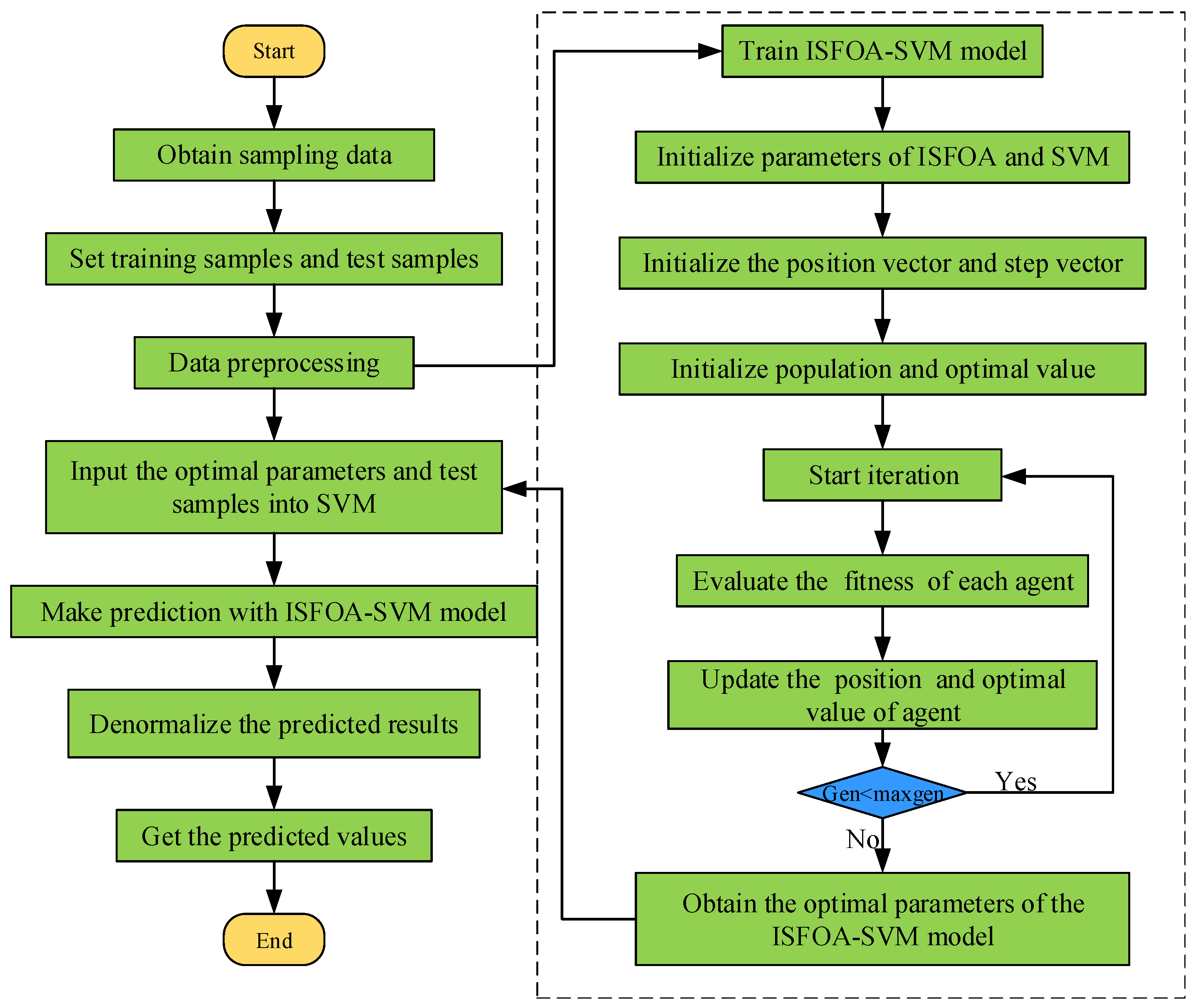
Figure 5 shows the overall structure of the ISFOA-SVM model for short-term wind power forecasting. The prediction process includes several key steps: data input, parameter optimization, model training, and prediction output. This process reflects the collaborative working mechanism between the ISFOA algorithm and the SVM model.

5.2. Results and Discussions

In order to verify the performance of the ISFOA-SVM model, the SFOA-SVM model, PSO-SVM model, MFO-SVM model, and GWO-SVM model are used to predict the wind power of the same sample points.

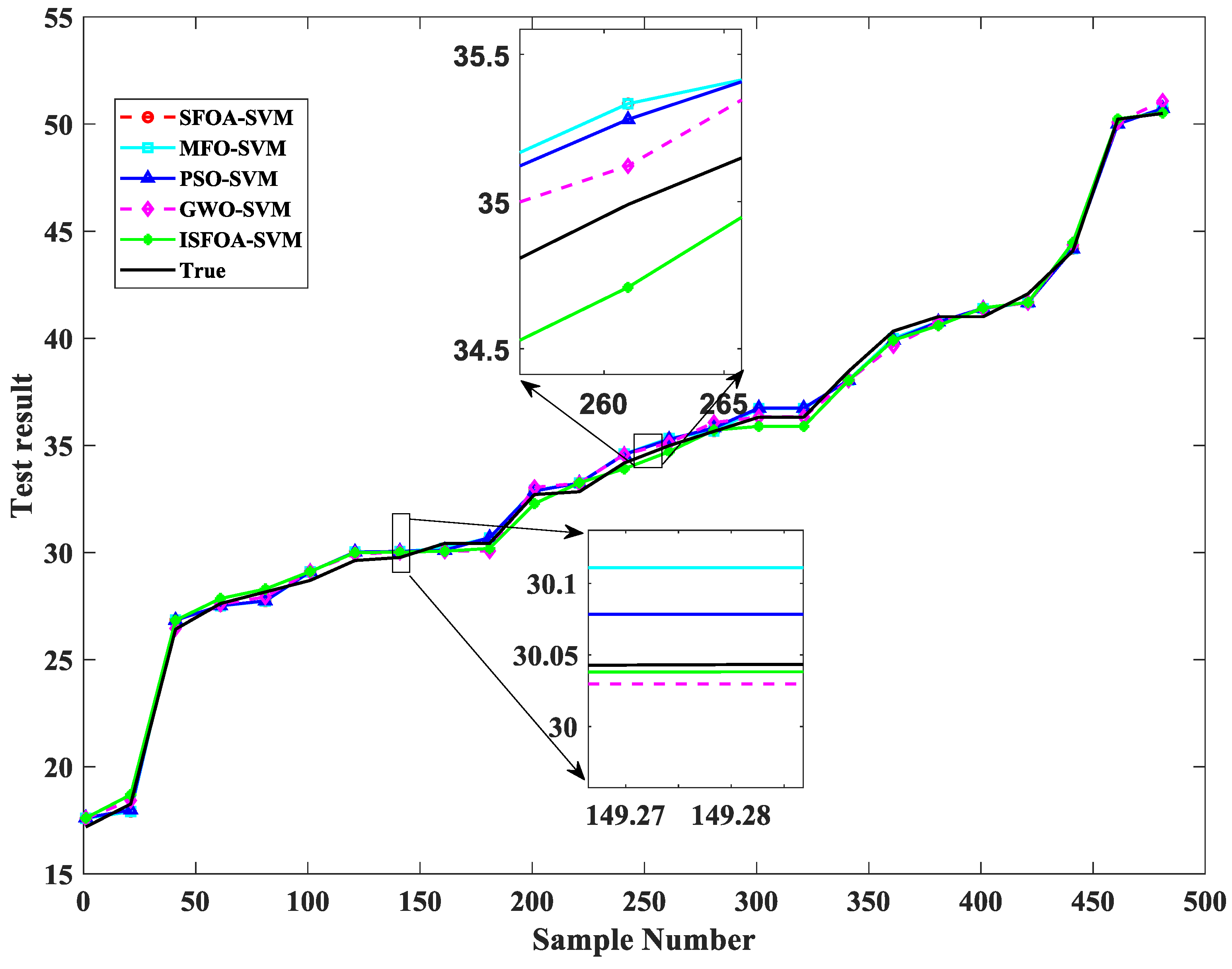
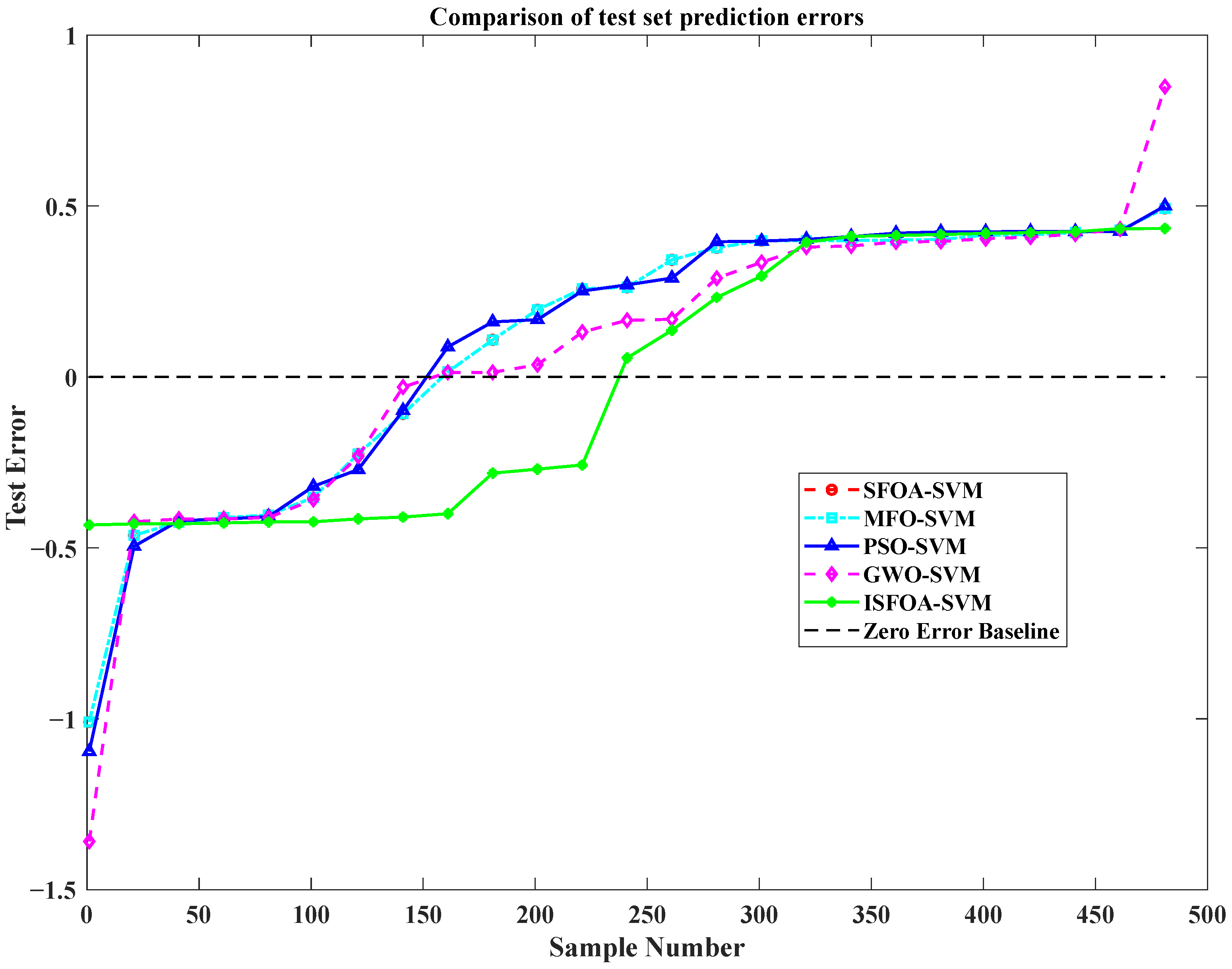
Figure 6 presents the prediction results of five algorithms (SFOA-SVM, PSO-SVM, MFO-SVM, GWO-SVM, and ISFOA-SVM) on the test set as the sampling points change, including two zoomed-in subplots. To compare the advantages and disadvantages of different algorithms, the test results in the figure are sorted from smallest to largest. The figure adopts a line chart format, with the horizontal axis representing the sampling points and the vertical axis representing the test set predicted values. Different algorithms are distinguished by colors, line types, and marker points: SFOA-SVM is marked with red dashed lines and circle markers, MFO-SVM uses cyan solid lines and square markers, PSO-SVM is represented by blue solid lines and upward triangle markers, GWO-SVM is shown with magenta dashed lines and diamond markers, and the proposed ISFOA-SVM in this paper is denoted by green solid lines and star markers. In addition, the zero error baseline is indicated by a black dashed line. In the figure, the test errors are sorted from smallest to largest and presented in the form of a line chart, where the horizontal axis represents the sampling points and the vertical axis represents the predicted values of the test set. All five algorithms can effectively predict the actual wind power values, but obvious differences can be observed through the detailed comparison of the two zoomed-in subplots. Specifically, the predicted values of the proposed ISFOA-SVM model have a higher consistency with the true values, demonstrating superior prediction accuracy.

Figure 7 compares the prediction errors of the five algorithms on the test set. As can be seen from the comparison, ISFOA-SVM has a lower proportion of large-error samples, and its overall error distribution tends to be at the intermediate level, maintaining a consistent advantage in prediction error among the five algorithms.

Table 4. The evaluation indexes of the prediction and test results.

	SFOA-SVM	PSO-SVM	MFO-SVM	GWO-SVM	ISFOA-SVM
MAE	0.3193	0.3378	0.3619	0.7456	0.3158
MBE	0.0278	0.0331	0.0342	0.0173	0.0126
RMSE	1.0038	0.3902	0.4142	0.5621	0.3304
R2	0.9948	0.9975	0.9973	0.9820	0.9982

The underlined data correspond to the optimal values in each row.

presents the performance of five algorithms—SFOA-SVM, PSO-SVM, MFO-SVM [33], GWO-SVM [34], and ISFOA-SVM—across four metrics: MAE, MBE, RMSE, and R², with the best value in each row underlined. Compared to SFOA-SVM, ISFOA-SVM improves MAE from 0.3193 to 0.3158 (approximately 1.10% improvement), MBE from 0.0278 to 0.0126 (approximately 54.68% improvement), RMSE from 1.0038 to 0.3304 (approximately 67.08% improvement), and R² from 0.9948 to 0.9982 (approximately 0.34% improvement). ISFOA-SVM achieves the best results in all four metrics, indicating smaller prediction errors and higher goodness-of-fit, with its overall performance significantly outperforming other algorithms. Among the comparative models, GWO-SVM shows relatively better performance in MBE (0.0173) compared to SFOA-SVM, PSO-SVM, and MFO-SVM, but it exhibits the worst performance in MAE, RMSE, and R². PSO-SVM and MFO-SVM exhibit intermediate results across all metrics.

6. Conclusions

This study focuses on addressing key challenges in short-term wind power prediction and achieves significant improvements in prediction performance through algorithm optimization and model integration strategies. The main conclusions are as follows:

An improved superb fairy-wren optimization algorithm (ISFOA) is proposed. This algorithm dynamically adjusts the search step size by introducing an adaptive learning factor, which enhances the ability to explore global optimal solutions and effectively avoids falling into local optima. Meanwhile, it integrates a differential evolution strategy to optimize the local search process, significantly accelerating convergence speed and improving optimization accuracy. Convergence analysis based on the Markov chain model verifies the stability and reliability of the ISFOA optimization process.

For the actual power prediction task of a wind farm in southern China, the ISFOA is integrated with Support Vector Machine (SVM) to construct the ISFOA-SVM model, and its performance is evaluated against four comparative models: SFOA-SVM, PSO-SVM, MFO-SVM, and GWO-SVM. The results demonstrate that ISFOA-SVM achieves the best performance across all evaluation metrics. Compared with the original SFOA-SVM, all key error indicators are significantly optimized: the Root Mean Square Error (RMSE) shows a substantial reduction of 67.08%; the Mean Bias Error (MBE) is optimized by approximately 54.68%; and the Mean Absolute Error (MAE) and coefficient of determination (R²) are improved by 1.10% and 0.34%, respectively. Among all comparative models, ISFOA-SVM ranks first with the lowest error levels and the highest goodness-of-fit (R² = 0.9982), and its comprehensive performance is significantly superior to other models, fully confirming its effectiveness in short-term wind power prediction.

However, the ISFOA-SVM model still has limitations: its prediction performance relies on the regression capability of SVM, and when processing large-scale datasets, prediction accuracy may decrease due to the high computational complexity of SVM. Future research will focus on exploring alternative models (such as Least Squares Support Vector Machine (LSSVM) and Grey Model) and further optimizing model integration strategies to enhance the model’s adaptability and stability in complex scenarios.

References

1. Jiao, R.; Huang, X.; Ma, X.; Han, L.; Tian, W. A Model Combining Stacked Auto Encoder and Back Propagation Algorithm for Short-Term Wind Power Forecasting. IEEE Access 2018, 6, 17851–17858. [Google Scholar] [CrossRef]
2. Zhang, J.; Cui, M.; Hodge, B.M.; Florita, A.; Freedman, J. Ramp forecasting performance from improved short-term wind power forecasting over multiple spatial and temporal scales. Energy 2017, 122, 528–541. [Google Scholar] [CrossRef]
3. Ji, S.; Zhang, L.; Wang, J.; Wei, T.; Li, J.; Ling, B.; Xu, J.; Wu, Z. Short-Term Power Load Forecasting Based on DPSO-LSSVM Model. IEEE Access 2025, 13, 32211–32224. [Google Scholar] [CrossRef]
4. Hu, X.; Li, H.; Si, C. Improved composite model using metaheuristic optimization algorithm for short-term power load forecasting. Electr. Power Syst. Res. 2025, 241, 111330. [Google Scholar] [CrossRef]
5. Zheng, G.; Kong, L.; Su, Z.; Hu, M.; Wang, G. Approach for Short-Term Power Load Prediction Utilizing the ICEEMDAN–LSTM–TCN–Bagging Model. J. Electr. Eng. Technol. 2025, 20, 231–243. [Google Scholar] [CrossRef]
6. Tang, C.; Zhang, Y.; Wu, F.; Tang, Z. An Improved CNN-BILSTM Model for Power Load Prediction in Uncertain Power Systems. Energies 2024, 17, 2312. [Google Scholar] [CrossRef]
7. Wan, S.; Wang, Y.; Zhang, Y.; Zhu, B.; Huang, H.; Liu, J. Fusion of Hierarchical Optimization Models for Accurate Power Load Prediction. Sustainability 2024, 16, 6903. [Google Scholar] [CrossRef]
8. Li, J.; Wen, M.; Zhou, Z.; Wen, B.; Yu, Z.; Liang, H.; Zhang, X.; Qin, Y.; Xu, C.; Huang, H. Multi-objective optimization method for power supply and demand balance in new power systems. Int. J. Electr. Power Energy Syst. 2024, 161, 110204. [Google Scholar] [CrossRef]
9. Geng, G.; He, Y.; Zhang, J.; Qin, T.; Yang, B. Short-Term Power Load Forecasting Based on PSO-Optimized VMD-TCN-Attention Mechanism. Energies 2023, 16, 4616. [Google Scholar] [CrossRef]
10. Abad Santjago, A.; Pelaez, C.; Perez-Aracil, J.; Sanz Justo, J.; Casanova Mateo, C.; Salcedo Sanz, S. Hybridizing Machine Learning Algorithms With Numerical Models for Accurate Wind Power Forecasting. Expert Syst. 2025, 42, e13830. [Google Scholar] [CrossRef]
11. Mansoor, M.; Tao, G.; Mirza, A.F.; Irfan, M.; Chen, W. Feature fusion temporal convolution: Wind power forecasting with light hyperparameter optimization. Energy Rep. 2025, 13, 2468–2481. [Google Scholar] [CrossRef]
12. Gao, Y.; Xing, F.; Kang, L.; Zhang, M.; Qin, C. Ultra-Short-Term Wind Power Forecasting Based on DT-DSCTransformer Model. IEEE Access 2025, 13, 22919–22930. [Google Scholar] [CrossRef]
13. Wang, H.; Peng, C.; Liao, B.; Cao, X.; Li, S. Wind Power Forecasting Based on WaveNet and Multitask Learning. Sustainability 2023, 15, 10816. [Google Scholar] [CrossRef]
14. Zhao, Z.; Bai, J. Ultra-Short-Term Wind Power Forecasting Based on the MSADBO-LSTM Model. Energies 2024, 17, 5689. [Google Scholar] [CrossRef]
15. Khamari, R.C.; Mani, S.; Bodkhe, R.G.; Singh, A.K. Enhancing wind power forecasting accuracy: A hybrid SNGF-RERNN-SCSO approach. Sol. Energy 2025, 295, 113513. [Google Scholar] [CrossRef]
16. Konstantinou, T.; Hatziargyriou, N. Regional Wind Power Forecasting Based on Bayesian Feature Selection. IEEE Trans. Power Syst. 2025, 40, 113–124. [Google Scholar] [CrossRef]
17. Zhang, J.; Zhao, Z.; Yan, J.; Cheng, P. Ultra-Short-Term Wind Power Forecasting Based on CGAN-CNN-LSTM Model Supported by Lidar. Sensors 2023, 23, 4369. [Google Scholar] [CrossRef] [PubMed]
18. Ma, W.; Zhang, X.; Xin, Y.; Li, S. Study on short-term network forecasting based on SVM-MFA algorithm. J. Vis. Commun. Image Represent. 2019, 65, 102646. [Google Scholar] [CrossRef]
19. Zhang, S.; Zhang, N.; Zhang, Z.; Chen, Y. Electric Power Load Forecasting Method Based on a Support Vector Machine Optimized by the Improved Seagull Optimization Algorithm. Energies 2022, 15, 9197. [Google Scholar] [CrossRef]
20. Li, W.; Tang, J.; Ma, H.; Fan, M.; Liu, S.; Wang, J. Load Prediction Based on Optimization Ant Colony Algorithm. J. Electr. Eng. Technol. 2023, 18, 27–37. [Google Scholar] [CrossRef]
21. Samantaray, S.; Sahoo, A. Prediction of suspended sediment concentration using hybrid SVM-WOA approaches. Geocarto Int. 2021, 37, 5609–5635. [Google Scholar] [CrossRef]
22. Hooshmand, F.; Seilsepour, F.; MirHassani, S. Adjustable robust optimization approach for SVM under uncertainty. Omega 2025, 131, 103206. [Google Scholar] [CrossRef]
23. Mahmoud, A.M.; Lashin, M.M.A.; Alrowais, F.; Karamti, H. A Dual Soft-Computing Based on Genetic Algorithm and Fuzzy Logic Defect Recognition for Gearbox and Motors: Attempts Toward Optimal Performance. IEEE Access 2022, 10, 73956–73968. [Google Scholar] [CrossRef]
24. Kouachi, S.; Bourouba, N.; Mebarkia, K.; Laidani, I. Analog Circuits Fault Diagnosis Using ISM Technique and a GA-SVM Classifier Approach. Electron. ETF 2024, 28, 54–67. [Google Scholar] [CrossRef]
25. Shojae Chaeikar, S.; Manaf, A.A.; Alarood, A.A.; Zamani, M. PFW: Polygonal Fuzzy Weighted—An SVM Kernel for the Classification of Overlapping Data Groups. Electronics 2020, 9, 615. [Google Scholar] [CrossRef]
26. Jia, H.; Zhou, X.; Zhang, J.; Mirjalili, S. Superb Fairy-wren Optimization Algorithm: A novel metaheuristic algorithm for solving feature selection problems. Clust. Comput. 2025, 28, 246. [Google Scholar] [CrossRef]
27. Chen, L.; Zhang, S.; Qin, Y.; Cao, K.; Du, T.; Dai, Q. Software defect prediction based on support vector machine optimized by reverse differential chimp optimization algorithm. Int. J. Data Sci. Anal. 2025. [Google Scholar] [CrossRef]
28. Rodan, A.; Al-Tamimi, A.K.; Al-Alnemer, L.; Mirjalili, S.; Tiňo, P. Enzyme action optimizer: A novel bio-inspired optimization algorithm. J. Supercomput. 2025, 81, 686. [Google Scholar] [CrossRef]
29. Xiong, Y.; Cheng, J. A Modified Sine Cosine Algorithm for Numerical Optimization. Int. J. Comput. Intell. Appl. 2024, 23, 2450015. [Google Scholar] [CrossRef]
30. Jia, H.; Zhou, X.; Zhang, J.; Abualigah, L.; Yildiz, A.R.; Hussien, A.G. Modified crayfish optimization algorithm for solving multiple engineering application problems. Artif. Intell. Rev. 2024, 57, 127. [Google Scholar] [CrossRef]
31. Kameyama, K. Particle Swarm Optimization-A Survey. IEICE Trans. Inf. Syst. 2009, E92-D, 1354–1361. [Google Scholar] [CrossRef]
32. Wu, F.; Zhou, Z.; Guo, Y. Hybrid-Driven Car-Following Model Based on Improved Composite Network and IDM. Arab. J. Sci. Eng. 2025, 50, 741–757. [Google Scholar] [CrossRef]
33. Mirjalili, S. Moth-flame optimization algorithm: A novel nature-inspired heuristic paradigm. Knowl.-Based Syst. 2015, 89, 228–249. [Google Scholar] [CrossRef]
34. Mirjalili, S.; Mirjalili, S.M.; Lewis, A. Grey Wolf Optimizer. Adv. Eng. Softw. 2014, 69, 46–61. [Google Scholar] [CrossRef]
Figure 1. Schematic diagram of the support vector regression prediction process.
Electronics 14 03172 g001
Figure 2. The flowchart of the improved superb fairy-wren optimization algorithm.
Electronics 14 03172 g002
Figure 3. Convergence curves of 6 algorithms with CEC2022 in 20 dimensions.
Electronics 14 03172 g003
Figure 4. Boxplot of 6 algorithms with CEC2022 in 20 dimensions.
Electronics 14 03172 g004
Figure 5. Flow chart of ISFOA-SVM for short-term wind power prediction.
Electronics 14 03172 g005
Figure 6. Prediction results comparison for five algorithms on the test set.
Electronics 14 03172 g006
Figure 7. Comparison of test errors for five algorithms.
Electronics 14 03172 g007