Article

Novel Adaptive Intelligent Control System Design

1
Department of Robotics and Computational Intelligence Systems, School of Engineering, King Mongkut’s Institute of Technology Ladkrabang, Bangkok 10520, Thailand
2
Department of Robotics and AI Engineering, School of Engineering, King Mongkut’s Institute of Technology Ladkrabang, Bangkok 10520, Thailand
3
School of Integrated Technology, Yonsei University, Incheon 21983, Republic of Korea
4
Medical Imaging & Intelligent Reality Lab, Convergence Medicine Asan Medical Center, Seoul 05505, Republic of Korea
*
Author to whom correspondence should be addressed.
Electronics 2025, 14(15), 3157; https://doi.org/10.3390/electronics14153157
Submission received: 30 June 2025 / Revised: 27 July 2025 / Accepted: 4 August 2025 / Published: 7 August 2025
(This article belongs to the Special Issue Nonlinear Intelligent Control: Theory, Models, and Applications)

Abstract

A novel adaptive intelligent control system (AICS) with learning-while-controlling capability is developed for a highly nonlinear single-input single-output plant by redesigning the conventional model reference adaptive control (MRAC) framework, originally based on first-order Lyapunov stability, and employing customized neural networks. The AICS is designed with a simple structure, consisting of two main subsystems: a meta-learning-triggered mechanism-based physics-informed neural network (MLTM-PINN) for plant identification and a self-tuning neural network controller (STNNC). This structure, featuring the triggered mechanism, facilitates a balance between high controllability and control efficiency. The MLTM-PINN incorporates the following: (I) a single self-supervised physics-informed neural network (PINN) without the need for labelled data, enabling online learning in control; (II) a meta-learning-triggered mechanism to ensure consistent control performance; (III) transfer learning combined with meta-learning for finely tailored initialization and quick adaptation to input changes. To resolve the conflict between streamlining the AICS’s structure and enhancing its controllability, the STNNC functionally integrates the nonlinear controller and adaptation laws from the MRAC system. Three STNNC design scenarios are tested with transfer learning and/or hyperparameter optimization (HPO) using a Gaussian process tailored for Bayesian optimization (GP-BO): (scenario 1) applying transfer learning in the absence of the HPO; (scenario 2) optimizing a learning rate in combination with transfer learning; and (scenario 3) optimizing both a learning rate and the number of neurons in hidden layers without applying transfer learning. Unlike scenario 1, no quick adaptation effect in the MLTM-PINN is observed in the other scenarios, as these struggle with the issue of dynamic input evolution due to the HPO-based STNNC design. Scenario 2 demonstrates the best synergy in controllability (best control response) and efficiency (minimal activation frequency of meta-learning and fewer trials for the HPO) in control.

1. Introduction

Traditional control algorithms often struggle to efficiently manage intricate nonlinear systems. This study proposes a novel adaptive intelligent control system (AICS) as an alternative to the conventional model reference adaptive control (MRAC) system [1], which is restricted in effectively controlling highly nonlinear systems. A higher-order Lyapunov function may serve as a viable solution for enhancing the MRAC system’s performance by offering greater adaptive flexibility. Additionally, combining the MRAC with traditional control systems such as PID control, H∞ control, sliding mode control, and others can be considered as alternative approaches. However, it is important to note that not only the analytical discovery of the Lyapunov function but also the design of the hybrid control systems require extensive expertise in mathematics and control theory. This highlights the necessity of advanced intelligent control frameworks to address these challenges.
The key advantages, including a highly parallel architecture, adaptability, nonlinear mapping capability, and robustness, strongly encourage the use of neural networks for nonlinear system identification and/or control. According to a paper [2], the term “intelligent control” was first introduced in the 1970s. Since then, diverse intelligent control systems have gained considerable attention in modern engineering applications for their potential to address challenges posed by highly nonlinear and intricate dynamic processes. Branches in intelligent control include neural network (NN)-based control, fuzzy control, genetic algorithm-based control, planning system-based control, expert system-based control, and hybrid system-based control, all of which are active research areas. This paper offers the literature review of NN-based control strategies that incorporate either a neural network-based plant identifier [1,3], a neural network controller [4,5,6,7,8,9], or both [10,11,12,13,14,15,16,17]. Most studies [1,3,4,5,6,7,9,13,16] permitted online learning, but some [8,11,17] did not. Studies [1,7,11,15,16,17] explored single-input single-output (SISO) plants, while another [3] focused on multiple-input multiple-output plants. One study [13] handled both. Their applications primarily targeted the diverse branches of robotics [4,5,6,9]. A study [9] tested an inverted pendulum, a cartpole, a vehicle, a pendubot, and a power system with recurrent NN-based controllers. From the perspective of algorithmic principles, NN-based intelligent control can be categorized into the following: (I) adaptive control [1,4,5,6,7,8,12,13,15,16,17]; (II) adaptive inverse control [10]; (III) internal model control [11,12]; (IV) predictive control [12]; (V) adaptive critic control [14]; (VI) reinforcement learning-based control [12]. Secondary considerations, which can be challenging and may require extensive simulations, could be viewed as potential weaknesses, complicating control system design and impacting control performance. The following are some examples: adaptation laws [1]; a fictitious controller [4]; subsystems for generating an auxiliary term to adjust a control signal [7]; a robustness filter for plant-model mismatch [11,12] and control law [11] in (III); a numerical optimization routine [12] in (IV); and control and feedback laws [15]. Ultimately, the aforementioned studies [1,4,7,11,12,15] required one or more additional subsystems to implement their control strategies, which are redundant for the proposed AICS. Studies [18,19] using reinforcement learning based on rewards and penalties inherently exhibit a trial-and-error nature. This can lead to risky behaviours during exploration with potentially harmful consequences, particularly in critical real-world applications based on online learning-while-controlling. Despite significant progress in safety from recent studies [20,21,22,23], reinforcement learning-based approaches may not provide a fundamental solution. Q-learning [24,25,26] can help mitigate the risk, but it is not expected to fully eliminate the issue either. This study develops the AICS, categorized under (I), through the redesign of the MRAC system based on first-order Lyapunov stability, as it incorporates customized neural networks to integrate and replace subsystems in the MRAC system.
In intelligent control system design, domain knowledge [2] is essential for the following: (a) plant modelling; (b) design of a controller with adaptive parameters; (c) adaptation of a control system to a changing environment; (d) acquisition of new design objectives and constraints; (e) stability verification of a proposed control system. The AICS consists of two main subsystems: a meta-learning-triggered mechanism-based physics-informed neural network (MLTM-PINN) for online plant identification and a self-tuning neural network controller (STNNC). To address (a), this study designs the MLTM-PINN based on the findings from an earlier study [1], integrating several innovative techniques: each PINN trained online through self-supervised learning without the need for labelled data; a meta-learning process activated by a triggered mechanism for consistent fine adaptation; transfer learning combined with meta-learning for finely customized initialization and quick adaptation to input changes. Raissi et al. [27] made significant advancements in PINNs. Their success has motivated many researchers to explore similar approaches [28,29,30,31,32,33,34,35] across various branches of applied mathematics, science, and engineering. Robinson et al. [35] attempted a new method for integrating domain knowledge during training. However, they were unable to generalize their integration method due to the different modelling nature of benchmark problems. This study instead uses regularization, which streamlines the structure of PINNs. When it comes to meta-learning, Hochreiter et al. [36] and Younger et al. [37] signified a pivotal moment. A gradient-based model-agnostic meta-learning (MAML) model [38] used in this study marked a notable advancement in learning algorithms with multiple inner learners and a single outer learner for further adjustment. Since then, various ideas [39,40,41] based on the MAML, aimed at enhancing meta-learning algorithms, have emerged. The MAMLs offer key advantages over metric- and model-based approaches. It is model-agnostic and applicable to any differentiable model for tasks in supervised, self-supervised, and reinforcement learning. Unlike metric- and model-based methods, they support direct parameter adaptation via gradient updates without relying on task-specific model structures and prior knowledge of system dynamics, enhancing generalization, especially in few-shot or domain-shift settings. It integrates efficiently with standard optimization workflows and scales, making it both flexible and effective. To avoid a decline in control performance, some studies [42,43] opted to use labelled data for a PINN, even if it was minimal, and another study [44] addressed boundary value problems, inherently reducing the usage of labelled data. In designing control systems, meta-learning was tested for quick adaptation and/or finely tailored initialization [45,46,47,48]. Transfer learning facilitated computational speed-ups by initializing subnetworks [1,49]. The study [1] by Duanyai was the first attempt to integrate the MAML, PINNs, and transfer learning in control.
This study highlights (b) by designing the STNNC with online adaptive parameters. It functionally integrates the nonlinear controller and adaptation laws in the MRAC system. This integration streamlines the AICS structure while retaining high controllability and control efficiency. To evaluate and compare control performances, three distinct scenarios are explored, each employing a different STNNC design approach with either transfer learning, hyperparameter optimization (HPO), or a combination of both. Bayesian optimization (BO) is a type of black-box optimization [50] that operates without explicit knowledge of an objective function’s internal structure. This study employs a Gaussian process tailored for BO (GP-BO), which is particularly efficient in low-dimensional hyperparameter spaces. Traditional optimization methods, such as grid search and random search, often struggle with highly nonlinear system dynamics. In contrast, GP-BO learns complex patterns and relationships in data, enabling more efficient navigation of a hyperparameter search space. It offers several advantages, including sample efficiency, adaptive search, uncertainty quantification, the intelligent balance between exploration and exploitation, applicability across continuous, discrete, and categorical hyperparameter spaces, and effectiveness in global optimization. The core idea of BO is to model an unknown objective function using a surrogate model or a response surface model, each of which is used to determine the next evaluation point. This strategy can be traced back to the work of Kushner [51]. The work by Zhilinskas [52] and Močkus [53] built upon the research, but the efficient global optimization algorithm by Jones et al. [54] received greater attention. HPO in machine learning, contributed by Snoek et al. [55], has gained incredible popularity. Salemi et al. [56] and Mehdad and Kleijnen [57] advanced insight into GP-BO for system optimization, making it a practical tool for a wide range of applications. Booker et al. [58] and Regis and Shoemaker [59,60,61] explored surrogate methods. A study [59] noted that in gradient-based optimization (GDO), a well-known form of non-black-box optimization, derivatives are not always available, and finite-difference approximations can be too costly to perform. These shortcomings explain why GDO is not as popular as BO in HPO. GPs are commonly regarded as one of the representative surrogate models in BO [62,63,64]. A GP-BO process follows three steps: (1) definition of GP prior distribution; (2) acquisition of new sets of hyperparameters and the update of observed data relative to an underlying objective function; (3) update of GP posterior distribution. GP is fully characterized by a mean function and a covariance function. The choice of a kernel family was made manually in advance [65,66,67] or automatically [68]. Roman et al. [69] proposed adaptive kernel selection strategies for BO. In this study, a Matérn kernel with pre-tuned parameters [65] (see Equation (33)) is used. Acquisition functions include expected improvement (EI) [54,55,70], probability of improvement [70], upper confidence bound [55], Thompson sampling [71], and others. Močkus [53] introduced the fundamental concept of EI. This study employs EI (see Equation (34)) without requiring parameter tuning [55], effectively balancing exploration and exploitation.
In this study, one aspect of (d) involves the decision-making of the AICS in control, with a particular focus on the trade-off between high controllability and control efficiency. Scenario 2 identifies the best solution to the conflict. It enhances the predictive capability and the computational efficiency of the MLTM-PINN, providing qualitative feedback to the STNNC and receiving a high-quality input in return, as both subsystems seamlessly operate within the cohesive AICS. This exemplifies the best synergy achieved by the data-driven model in predicting the behaviour of the highly nonlinear plant and optimizing control actions. The series of our forthcoming studies (see Section 6) will address (c) adaptation to environmental changes using a denoising autoencoder and (e), which focuses on estimating the stability of a designed control system.

2. AICS Design Strategy and Motivation

This section introduces the design strategy of the AICS, which is derived from the traditional MRAC framework. Initially, we design the MRAC system based on first-order Lyapunov stability and then modify it to develop the AICS with two subsystems. This section tests the MRAC system to highlight its shortcomings and the motivation for proposing the AICS design.

2.1. First-Order Lyapunov Stability Analysis of the MRAC System for a Single SISO Plant

This section presents a rigorous mathematical model that underpins the theoretical framework for MRAC system design, followed by AICS design derived from the reconstruction of the MRAC system. We first examine the first-order Lyapunov-based nonlinear MRAC stability [1] for the adaptive control of a first-order plant with the initial condition u p 0 = 0 , described by the equation:
u ˙ p t = A p · u p t C p · f p t + B p · u t
here, A p   =   1.0, B p = 3.0 , C p   =   1.0, and f p t   =   ( u p t ) 2 are used for all examples throughout this study. (     ) ˙ implies the first derivative of     with respect to t , and (   ) t indicates the function of t . u t is a control input. Online plant identification is implemented by a differential equation (DE) solver (see Figure 1) when a governing differential equation is given by Equation (1). u p t represents an output from the plant. Let the desired output u m t   of the reference model also be specified by the first-order differential equation as follows:
u ˙ m t = A m · u m t C m · f m t + B m · r t
where A m = 4.0 > 0 , B m = 4.0 > 0 ,   C m = 0.0 , and f m t   = 0.0 indicate constants.
r t = 4   s i n ( 3 t )
is a reference signal. A control law in the form of
u t = a u t · u p t + a r t · r t + a f t · f p t
is established to achieve adaptive control, incorporating the adaptive feedback gains, a u t , a r t , and a f t . This results in closed-loop dynamics that allow for systematic feedback adjustments. Let the tracking error be
e t = u p t u m t
and the error of parameter estimation be
a ~ u t = a u t a u
a ~ r t = a r t a r
a ~ f t = a f t a f
here, a u , a r , and a f are constants. According to Barbalat’s lemma, the following set of adaptation laws is identified as
a ˙ u t = γ · e t · u p t
a ˙ r t = γ · e t · r t
a ˙ f t = γ · e t · f p t
where γ implies an arbitrary positive constant, representing adaptation gain. To identify adaptive parameters for the nonlinear controller, these adaptive feedback gains are updated by
a u t + t = a u t + a ˙ u t · t
a r t + t = a r t + a ˙ r t · t
a f t + t = a f t + a ˙ f t · t
which ensures the convergence of e t . Therefore, the dynamics of the tracking error,
e ˙ t = A m e t + B p ( a ~ u t · u p t + a ~ r t · r t + a ~ f t · f p t )
can be found by subtracting Equation (2) from Equation (1). The first-order Lyapunov function for the plant is proposed by
V e t , a ~ u t , a ~ r t , a ~ f t = 1 2 ( e t ) 2 + 1 2 γ B p ( a ~ u t 2 + a ~ r t 2 + a ~ f t 2 ) 0
of which the first derivative becomes
V ˙ e t , a ~ u t , a ~ r t , a ~ f t = A m e t 2 < 0 .
Equation (10) supports the boundness of the signals e t , a ~ u t , a ~ r t , and a ~ f t , thereby ensuring the boundness of e ˙ t , and therefore, the uniform continuity of V ˙ e t , a ~ u t , a ~ r t , a ~ f t . As a result, the MRAC system is globally stable, and the globally asymptotic convergence of e t is achieved by Barbalat’s lemma.
Figure 1. Structure modification from the MRAC system to the AICS. (A) MRAC system. (B) AICS.
Electronics 14 03157 g001

2.2. AICS Design Strategy Derived from the MRAC Framework

We could pursue three directions to enhance the performance of the MRAC system: (i) analytically discovering a higher-order Lyapunov function to ensure tracking dynamics within the MRAC framework; (ii) developing a hybrid control algorithm by combining the MRAC system with other methods; (iii) modifying the MRAC system by using functionally customized neural networks (see Figure 1). The design approach proposed in this paper falls into the third category.
This section proposes a transition design strategy from the MRAC system to the AICS, focusing on structural simplification while maintaining desired performance. Figure 1 depicts the design of the AICS through the integration and reconstruction of the MRAC’s subsystems.
L t θ , λ ; D t r c = 1 2 ( e t ) 2
is tracking loss, evaluated automatically. All online adaptive parameters in the STNNC are updated at each time t based on Equation (12), with no need for labelled data. θ indicates a set of model parameters, and λ indicates a hyperparameter vector. D t r c denotes the auto-created training set of { t , u m t } for the STNNC. An output u p t from the MLTM-PINN is evaluated at t , where t = { t 0 ,   t ,   2 t ,     ,   t ,     ,   T } indicates an entire input time set with the current t , the initial time t 0 = 0 and the terminal time T = 4.5 for operating the AICS. t   = 0.01, used in controlling both the MRAC system and the AICS, represents a time step. For running the AICS, all input samples of an automatically discretized sub-time span t s u b for t (see Figure 5) are sequentially input into the MLTM-PINN during each control cycle. x = { u p t ,   e t } represents a state vector for a two-dimensional state space R 2 , excluding the remaining constant variables in Equation (7), and serves as a feedback input to ensure the closed-loop dynamics. An initial input set at t   = 0 is defined by x 0   = { u p 0 , e 0 } for all scenarios.
To design the AICS by reorganizing the MRAC subsystems, the adaptation laws and the adaptive feedback gains for the nonlinear controller are functionally integrated into the STNNC with multiple online adaptive parameters, without requiring extensive control domain knowledge. The DE solver is upgraded to the MLTM-PINN. Additionally, the AICS directly sets the desired output u m t as given by
48 25 e 4 t 1 + e 4 t · c o s 3 t 4 3   e 4 t · s i n 3 t
rather than deriving it from Equation (2). This study proposes three distinct design scenarios through the transition design strategy and examines the controllability (best control response) and the control efficiency (minimal activation frequency of meta-learning and a small number of trials for the HPO) of the AICS across these scenarios.

2.3. Motivation Behind the AICS Design

The MRAC system with two pre-tuned parameters γ and B p is simulated for t 0 = 0 and t f = 6.0 using the sixth order Runge–Kutta method as the DE solver. The plant and the reference models from Section 2.1 are used.
As shown in Figure 2, the subfigures display control responses for the B p values of 1.5, 3.0, 6.0, and 12.0, with each graph depicting the system’s response at the pre-tuned γ values ranging from 0.1 to 10.0. All system responses indicate suboptimal adaptation either in the initial phase or throughout the entire control process. Even increasing the value of γ to 10.0 fails to mitigate the initial fluctuations in all control responses across all B p values. Figure 3 details a specific case with a wider range of γ at B p = 3.0. As the value of γ increases to 72.0, the response diverges without any improvement in controllability, showing the initial phase of divergence in subfigure (A). The findings suggest that the MRAC system faces limitations in controlling highly nonlinear plants, possibly due to a lack of adaptive parameters. Nonetheless, the discovery of a higher-order Lyapunov function to ensure tracking dynamics for traditional MRAC system design remains a significant challenge.

3. AICS Design

This section provides a comprehensive introduction to the algorithms underlying the MLTM-PINN and the STNNC. The theoretical foundations and computational mechanisms of each component are discussed in detail to highlight their roles within the overall AICS framework. Particular emphasis is placed on how these algorithms contribute to achieving adaptive control and plant identification in dynamic environments.

3.1. MLP and PINN

Traditional machine learning algorithms often face challenges in data generation, which poses a significant obstacle in many scientific and engineering domains. PINNs can address this issue by integrating physical laws, typically expressed as differential equations, into a training process. This advantage allows PINNs to make more reliable predictions with minimal or even no data. In this study, a single PINN is employed to create each τ (task) in the MLTM-PINN. Figure 4 displays the PINN architecture that connects a multilayer perceptron (MLP) to physics laws.
The PINN uses the MLP with L hidden layers, and their outputs can be represented by the following equation:
y [ l ] = σ l θ l · y [ l 1 ] + b l ,   for   l = 1 ,   2 ,   3 ,   ,   L
and here, σ l denotes an activation function in the l -th hidden layer. y [ 0 ] is represented by t for l = 1. u p t is evaluated by
u p t = θ [ L + 1 ] · y [ L ] .
A set of optimal model parameters is achieved by implementing
θ = arg   min θ R m   L θ ; D t r
where L θ ; D t r indicates total loss combining initial constraint loss L I and residual loss L R . A training dataset D t r includes t s u b (see Figure 5) at t as an input set without labelled data for the MLTM-PINN. ( · ) indicates optimal ( · ). R m means an m-dimensional real space. Each τ for the MLTM-PINN employs four hidden layers, each containing 256 NE (neurons). Unlike, the MLTM-PINN, the STNNC does not include the physical laws. An MLP with two inputs in an input layer, originally comprising two hidden layers, is used for the STNNC. The first hidden layer includes eight NE, while the second contains 256 NE when the HPO strategies are not involved. It is automatically trained by Equation (12) (see Figure 1). Initialization is performed by Variance Scaling for the MLTM-PINN with Swish activations, while the STNNC with Tanh activations uses an Xavier Uniform initializer. None of the layers are frozen during the training in applying transfer learning.
Figure 5. A discretized sub-time span at t = 3.0.
Electronics 14 03157 g005
In our proposed framework, the target unstable plant is identified by the MLTM-PINN using a differential equation, which serves as one of physical laws. f θ m ( t ) (a single meta-model) employing inner learners is trained to approximate the solution to this differential equation. To incorporate physical constraints, both L I and L R are used to enforce consistency with the physical laws.

3.2. MLTM-PINN Design

This section focuses on developing the MLTM-PINN for online plant identification. All τ s in the subsystem adhere to a specific discretization rule for each t s u b . Figure 5 depicts the sampling manner for this initial value problem (refer to Section 2) by randomly sampling an input sub-time span for f θ m ( t ) with samples more closely concentrated around its initial constraint. It demonstrates a discretization case with a total of 100 samples at t = 3.0, including one sample at each end. All t s u b s follow the same sampling manner, but the distribution of input samples for each τ varies throughout the entire control process.
As stated in a study [72], the combination of meta-learning and transfer learning provides finely tailored initial features to τ s. This enables inner learners to develop more adaptable features, thereby improving the output accuracy of a single meta-model through iterative fine-tuning. Algorithm 1 outlines the bi-level learning process of the MAML-based meta-learning for the MLTM-PINN with ten inner learners at t , using a limited-memory Broyden–Fletcher–Goldfarb–Shanno with box constraints (L-BFGS-B) optimization strategy. It is founded on the basic concept presented in a work [73] and the further evolved versions by studies [74,75]. The strategy is detailed in steps 1 to 7 below:
  Step 1: set   k = 0   and   m s   = 50 .   Step 2: set   θ ( l o ) θ k θ ( u p ) .   Step 3: compute   d k   by using two-loop recursion (17) set   q = g k (18) define   P θ k = m i n ( max θ ( l o ) , θ k , θ ( u p ) )   for   c = k   to   m a x ( 0 ,   k m s )   d o : this first loop iterates backwards (19a) compute   δ c ( 1 ) = ρ c · s c T · q   where (19b) ρ c = 1 y c T · s c (20) update   q q δ c 1 · y c   end   for (21) set   r = H k · q   for   c =   m a x 0 ,   k m s t o k   do : this second loop iterates forwards (22) compute   δ c ( 2 ) = ρ c · y c T · r (23) update   r r + s c ( δ c ( 1 ) δ c ( 2 ) )   end   for (24a) such   that   r H k · L θ k ; D t r   for each inner learner or (24b) r H k · L θ k ; D t r   for the outer learner (25) set   d k = r . (26) Step 4: perform   θ k + 1 = P ( θ k + k · d k ) (27a) compute   g k + 1 = L θ k + 1 ;   D t r   for each inner learner or (27b) g k + 1 = L θ k + 1 ;   D t r   for the outer learner, where a step size   k   is determined to satisfy Wolfe conditions without knowing   θ k + 1 . (28) Step 5: compute the memory   s k + 1 = θ k + 1 θ k   and (29) y k + 1 = g k + 1 g k   store the pairs ( s k + 1 ,   y k + 1 ), then remove the oldest pair to keep only the most recent   m s   pairs.   Step 6: let   m ~ =   m i n ( k ,   m s 1 )   and update Equation (30a) without storing its previous state. (30a) H k + 1 = ( V k T · · V k m ~ T ) H 0 ( V k m ~ T · · V k T )   +     ρ k m ~ ( V k T · · V k m ~ + 1 T )   s k m ~ · s k m ~ T ( V k m ~ + 1 T · · V k T )   +     ρ k m ~ + 1 ( V k T · · V k m ~ + 2 T )   s k m ~ + 1 · s k m ~ + 1 T ( V k m ~ + 2 T · · V k T )   +       +     ρ k · S k · S k T   where (30b) V k = I ρ k · y k · s k T   Step 7: update   k   k + 1   and go to step 3
where k indicates an iteration counter, and m s is the memory size, indicating how many previous updates are stored and used in the algorithm. θ ( l o ) and θ ( u p ) indicate lower and upper bounds, respectively. P ( · ) represents a projection function that keeps the iterations within the bounds. No bounds are applied to the L-BFGS-B in this study. δ c ( 1 ) refers to a step size for the backward process. H k denotes the approximation of an inverse Hessian matrix. δ c ( 2 ) refers to a step size for the forward process. Equation (24a,b) are aligned with the goal of the L-BFGS-B algorithm to maintain d k as the approximation of a search direction vector, which points toward the update direction of θ k , incorporating curvature information. L θ k ;   D t r and L θ k ;   D t r (or g k ) denote gradients. s k represents the difference between the successive sets of model parameters, and y k represents the difference between successive gradients. I refers to an identity matrix. H 0 is the initial approximation of H k .
Algorithm 1 MLTM-PINN algorithm
1:
input t
2:
create t sub
3:
initialize all required tensors and scalars
4:
create and sample f θ m ( t ) , τ s u s and τ q u s
5:
for  i t e r = 1 to i t e r m a x :
6:
  an initial θ 0 is used for i t e r = 1
7:
  initialize the first τ s u by using the updated θ of f θ m ( t ) : transfer learning
8:
for each τ s u do:
9:
    perform step 1 to step 7 using Equation (27a) to update each τ s u
10:
    if (C1) (C3):
11:
     break
12:
    initialize a following τ s u by using the updated θ of the current τ s u (except for the last τ s u ): transfer learning
13:
  initialize all τ q u s by using the θ of each corresponding τ s u : transfer learning
14:
for all τ q u s do:
15:
    perform step 1 to step 7 using Equation (27b) to update f θ m ( t )
16:
    if (C1) ⋁ (C2) ⋁ (C3):
17:
     break
18:
    else:
19:
     go to 5
20:
evaluate u p t = f θ m ( t ) at t
where τ s u implies a support task and τ q u implies a query task. (C1) i t e r = i t e r m a x , (C2) L θ ;   D t r   <   ε , and (C3) g k   < ε H are stopping criteria. i t e r is an iteration counter. i t e r max is a maximum iterative number: 5000 is used for each inner learner, and 50 is used for the outer learner. ε =   8.0 ×   10 4 and ε H =   2.22045 × 10 9 indicate convergence tolerance and loss reduction tolerance, respectively. The number of line search steps per iteration is limited to 50.

3.3. STNNC Design

This section proposes three different scenarios for designing the STNNC. The foundational ideas of scenarios 1 and 2 are derived from a study by Duanyai [76]. Scenario 1 employs the transfer learning alone between neighbouring control cycles. Scenario 2, in addition to that, leverages the GP-BO (refer to Algorithm 2) to adjust a single hyperparameter α (learning rate). Lastly, scenario 3 optimizes both α and the number of NE in each hidden layer without applying the transfer learning. The GP-BO determines λ (set of optimal hyperparameters) that minimizes Equation (12) during the training, based on the HPO configurations presented in Table 1.
Algorithm 2 with β (balancing parameter) intelligently explores target regions within the hyperparameter search space that are likely to yield better control performance, while also considering potentially optimal solutions. This algorithm implements the GP-BO using a nested approach (refer to Equation (31)). The STNNC uses an Adam optimizer. R n represents an n-dimensional real space.
θ = arg   min θ R m   L T ( θ , λ ; D t r c )   subjected   to   λ = arg   min λ R n   L T ( θ , λ ; D t r c )
Here, the objective function f λ = f ( λ 1 ,   λ 2 ,   . , λ n ) , defined by Equation (12) in the study, is modelled as a Gaussian process for the training set λ =   { λ 1 ,   λ 2 ,   . ,   λ n } T in a hyperparameter space. λ i indicates an individual hyperparameter, and n indicates the number of hyperparameters. m λ denotes a mean function, and K λ ,   λ denotes a covariance function, referred to as a Matérn kernel function. λ and λ imply different initial samples. In this study, a single initial input is considered to estimate the initial shape of f λ . A smoothness parameter ν   = 2.5 controls the smoothness of the function. Γ ( · ) refers to a gamma function. K ν ( · ) indicates a modified Bessel function. l s = 1.0 is a length scaling factor, controlling how quickly correlations decay over distance. E I identifies a new hyperparameter set λ n e w = { λ 1 n e w , λ 2 n e w ,   , λ n n e w } T , where its value is maximized. f λ b e s t serves as the best (minimal) function value at the currently best-known hyperparameter set λ b e s t . β = 2.6 controls the trade-off between the exploration and the exploitation. Φ ( · ) denotes a cumulative distribution function, and ϕ ( · ) denotes a probability density function. y represents the loss value defined in Equation (12). σ implies the standard deviation of noise in y . The GP-BO internally handles this parameter during the training. σ 2 indicates a parameter that is added to the diagonal of the kernel matrix as the expected amount of noise and influences the GP posterior distribution by adjusting its covariance structure. N denotes a normal distribution.
Algorithm 2 Bi-level optimization process for the GP-BO
  1: initialize   u p 0 = 0   and   e 0 = 0   as inputs   2: initialize   θ   and   λ   3: define GP prior distribution: (32)   define   f λ ~ G P m ( λ ) , K λ ,   λ ,     where (33)   K λ ,   λ = 2 1 ν Γ ( ν ) 2 ν l s λ λ ν K ν 2 ν l s λ λ   4: acquires   λ n e w   when the   EI   is maximized and evaluate   y (34)   define   E I λ n e w E max f λ b e s t + β f λ , 0     = f λ b e s t + β m ( λ )   Φ f λ b e s t + β m ( λ ) σ + σ · ϕ f λ b e s t + β m ( λ ) σ   for   σ > 0 0 for   σ = 0   5: if   f λ b e s t + β > f λ : exploration   6:             search for   λ n e w   where the maximized   EI   is observed in a target hyperparameter search space   7: else :   exploitation   8:             intensively exploring   λ n e w   in the vicinity of the best hyperparameter combination found so far to further improve   λ b e s t (35) 9: update   θ n e w θ α L ( θ , λ n e w ) θ   10: evaluate   u t   of the STNNC using   λ n e w   and   θ n e w   11: evaluate   e t   and   y   12: update GP posterior distribution (36a)   evaluate   f λ n e w y , λ , λ n e w ~ N m λ n e w , K λ n e w , λ n e w     where (36b)   m λ n e w = K λ n e w , λ K λ , λ + σ 2 I 1 y     and (36c)   K ( λ n e w , λ n e w ) = K λ n e w , λ n e w K λ n e w , λ K λ , λ + σ 2 I 1 K λ , λ n e w (37) 13: update   f λ n e w ~ G P m λ n e w , K ( λ n e w , λ n e w )   14: update   λ b e s t λ n e w   and   θ b e s t θ n e w   when   y   achieves     the   smallest   value   observed   so   far     15: if   trial   <   MTR :   16:               go to   4   17: else:   18:               break   19: update   λ λ b e s t   and   θ θ b e s t   20: choose the best   u t   computed using   λ   and   θ

4. Simulation Results and Discussion
In this section, the three scenarios are evaluated regarding the controllability and the control efficiency of the AICS through rigorous simulations and analyses. The results of these evaluations will provide insights into the strengths and weaknesses of each scenario, guiding the further refinements of the proposed control system. The simulations are performed on Windows 11 with TensorFlow 2.10.0 running in Python 3.9.21.
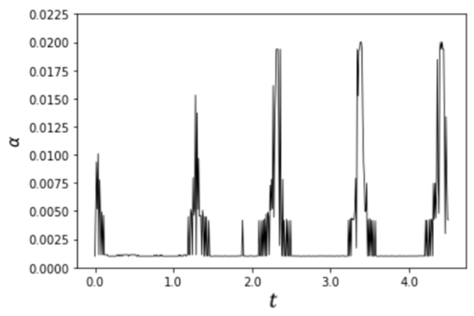
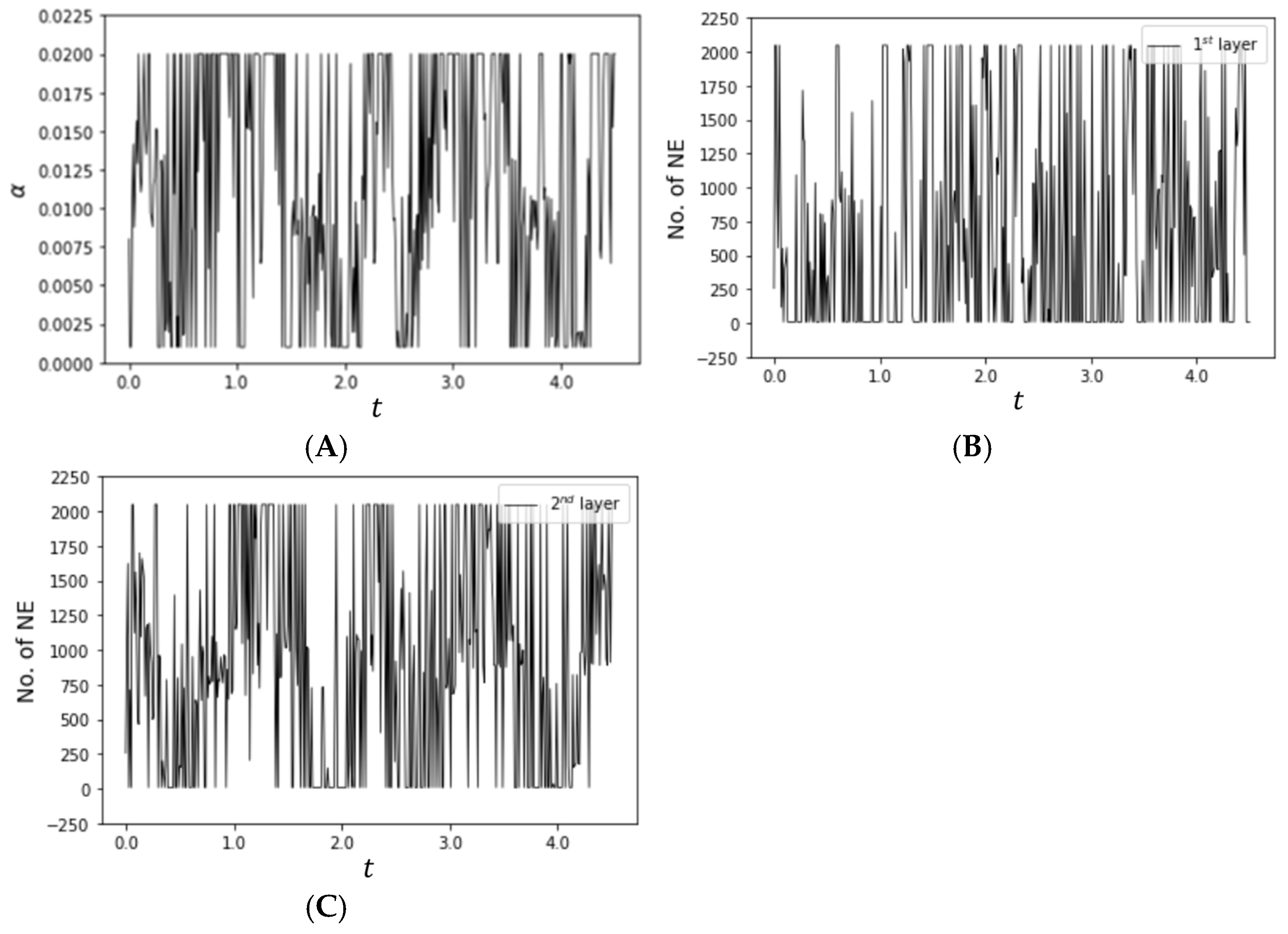
Figure 6 and Figure 7 visualize changes in the optimal values of the hyperparameters for scenarios 2 and 3. In Figure 6, scenario 2 illustrates that α fluctuates with several significant peaks, reaching the Max. V at the last two peaks, while the valleys attain the Min. V during the transitions. The upper bound appears adequate to cover all possible upper variations before the second-to-last peak, but the adequacy of the lower bound still remains uncertain. The transitions, marked by prolonged valleys, persist for extended durations rather than quickly rebounding. This could be interpreted as suggesting that the GP-BO algorithm continues to extensively explore the search space near the lower bound without being able to descend further, under the conditions of a single initial input point and MTR = 5. Nevertheless, the outputs in Figure 12 show that adjusting these three factors (the bounds, the number of initial samples, and the MTR) for the line search space is unnecessary. As depicted in Figure 7, the optimal hyperparameter values for scenario 3 wander with pronounced oscillations and no clear patterns, failing to gather sufficient data to accurately predict optimal values within the search space, which is constrained by inadequate bounds. Unlike in the 1D optimization case, a single initial input point in the 2D optimization may provide limited information about the objective function’s behaviour across the search space, thereby hindering the GP-BO from constructing an effective surrogate model from the outset. In addition, setting the MTR to 20 may also reduce the likelihood of finding better solutions. To observe discernible patterns in the variations, it is advisable to adjust the three factors by expanding the size of the hyperparameter search space, permitting more opportunities to explore it depending on its scale, and considering multiple initial samples. However, this solution is likely inefficient, as it requires additional computational resources, despite employing the fourfold larger MTR in scenario 3 compared to scenario 2 (see Table 1). It is easily expected that using multiple initial samples will lead to a longer search duration during the initial phase of the optimization.
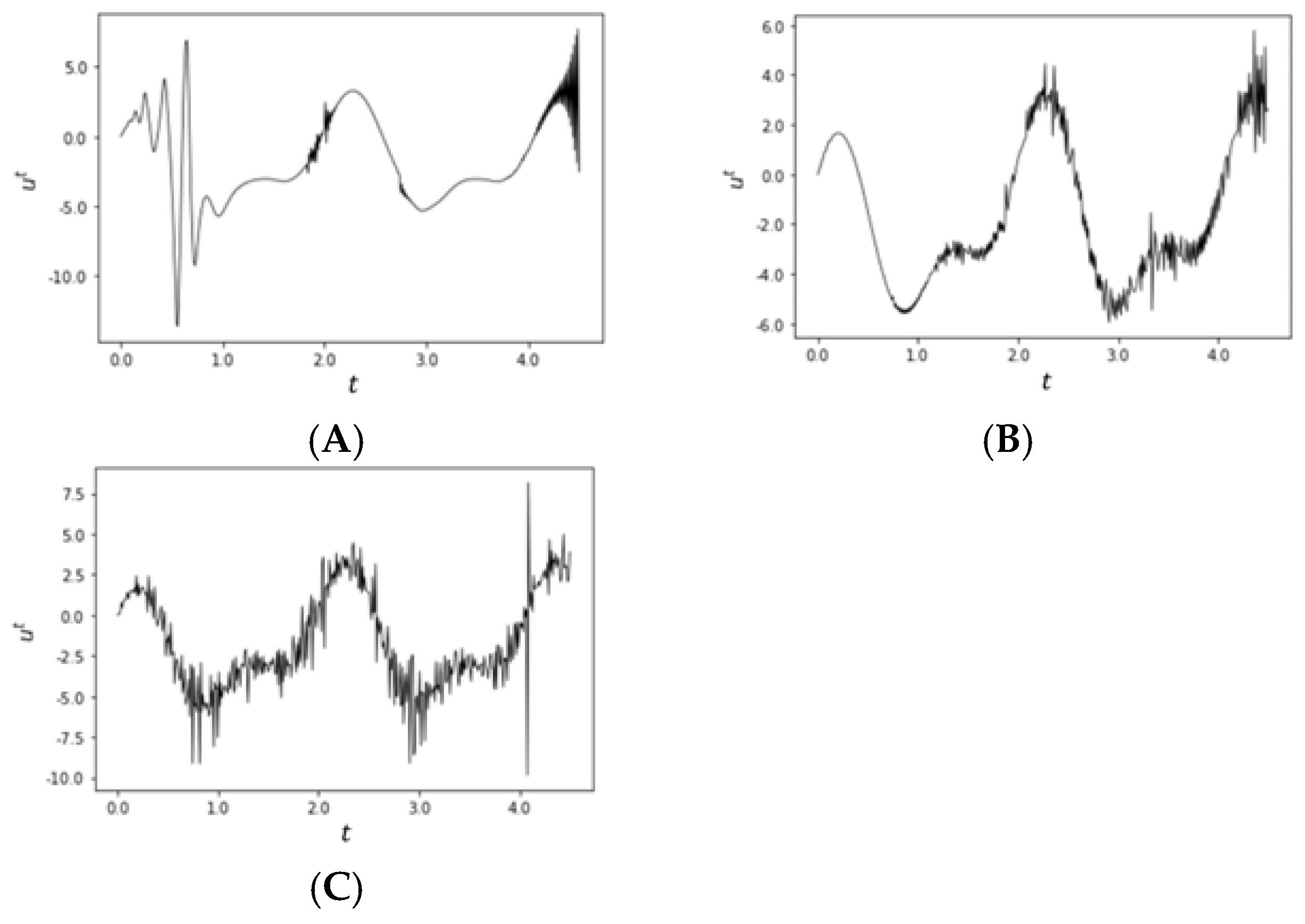
In Figure 8, unlike the other scenarios, scenario 1 has a different profile for u t that sets it apart. The distinct overall shape, along with the unstable portion observed at the end of the control process, reflects the inability of the STNNC to optimally compensate for the system’s dynamics, leading to the inferior tracking performance, as shown in Figures 11–13. In scenario 2, an increase in the micro-scale fluctuations, characterized by the formation of sharp spikes and drops, is observed after t = 0.8. These fluctuations are more obvious in scenario 3, which involves optimizing a greater number of hyperparameters. These findings suggest that the dynamic evolution of the u t inputs to the MLTM-PINN may contribute to its delayed adaptation (see Figure 10B,C).
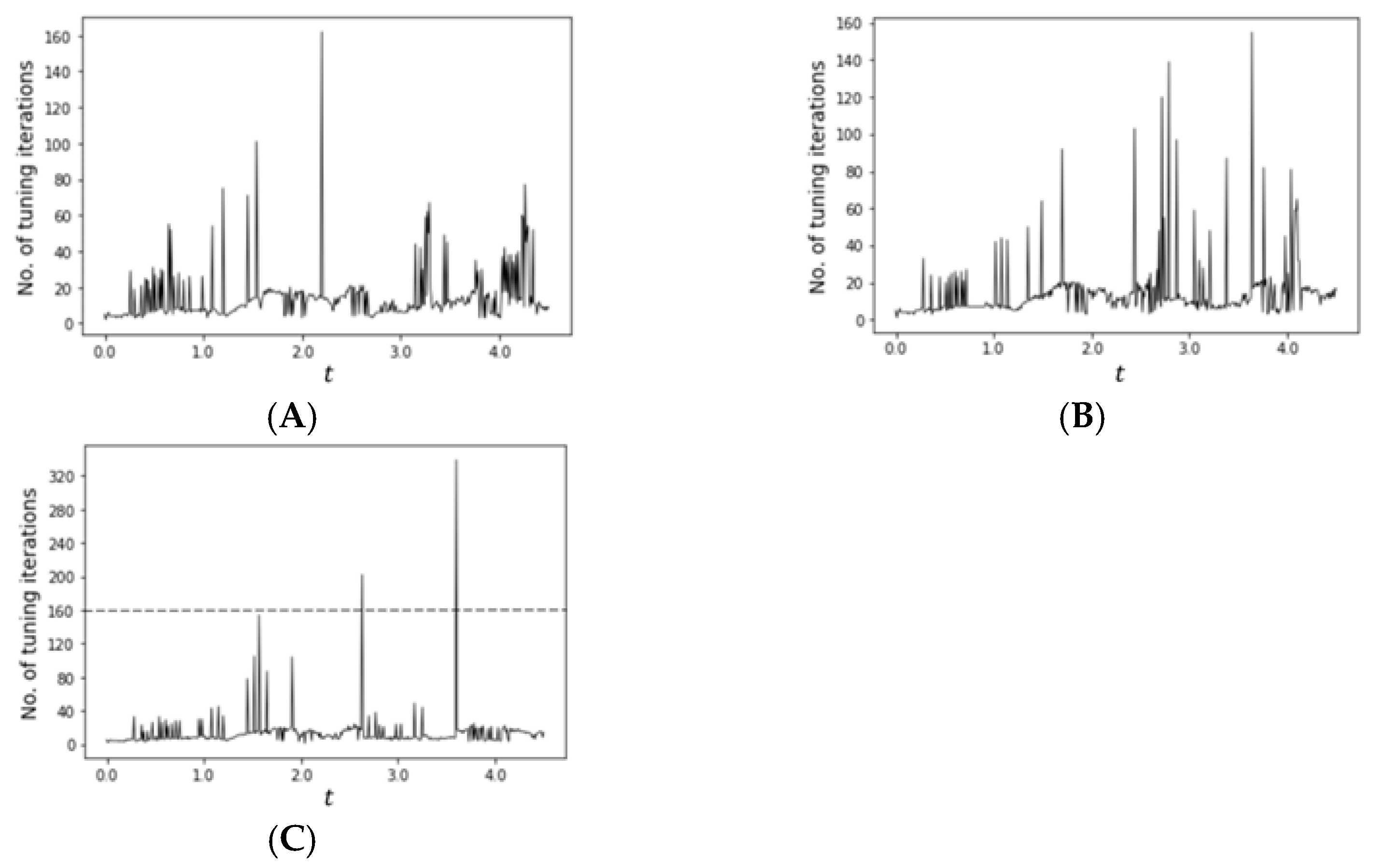
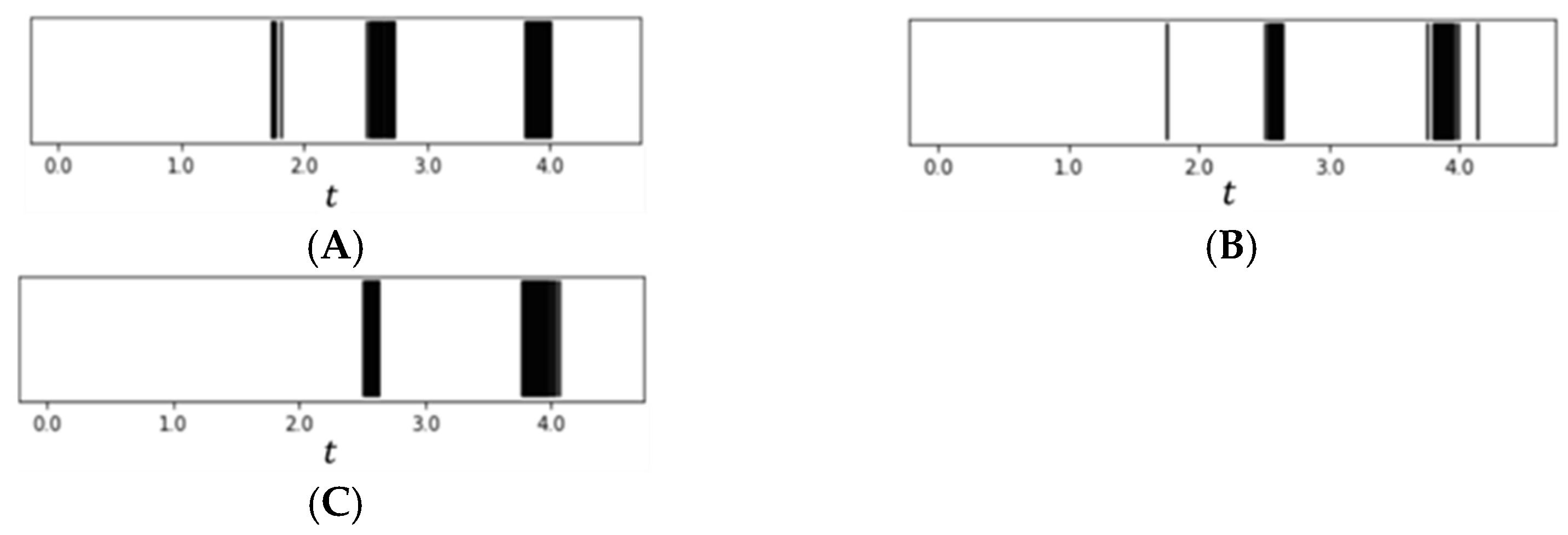
Figure 9, Figure 10, Figure 11, Figure 12 and Figure 13 illustrate changes in the performance of the MLTM-PINN and the AICS according to the distinct STNNC design scenarios. Figure 9 displays triggering event profiles across the scenarios. Scenario 2 triggers meta-learning the fewest number of times, totalling only 34 activations and indicating an advantage in minimizing computational demands. The findings from subfigures (B) and (C) highlight that achieving the high-quality tracking performances (see Figure 11, Figure 12 and Figure 13) necessitates activating it concentratedly after the midpoint of the control process. Figure 10 shows the training frequency of f θ m ( t ) for each scenario. As evidenced by the subfigures, a quick adaptation effect is observed in scenario 1 after the midpoint, despite its small magnitude. In contrast, no significant effect is observed in the other scenarios involving the HPO. Optimal hyperparameter settings in the STNNC may require further training for the MLTM-PINN to converge, as it slowly adapts to u t s with the dynamic input evolutions, which could alter the magnitude and direction of gradients in τ s for the MLTM-PINN in a manner different from scenario 1. According to the hypothesis, subfigure (C) in Figure 8 can also elucidate why subfigure (C) in Figure 10 illustrates the extended training duration in scenario 3. The observations point to the fact that the MLTM-PINN’s quick adaptation can be challenging when employing the HPO strategies for the STNNC design.
Figure 10. Changes in the training frequency of f θ m ( t ) across the scenarios. (A) Training frequency observed in scenario 1. (B) Training frequency observed in scenario 2. (C) Training frequency observed in scenario 3.
Electronics 14 03157 g010
Figure 11. Controllability of the AICS designed by scenario 1. (A) Control response. (B) Tracking error.
Electronics 14 03157 g011
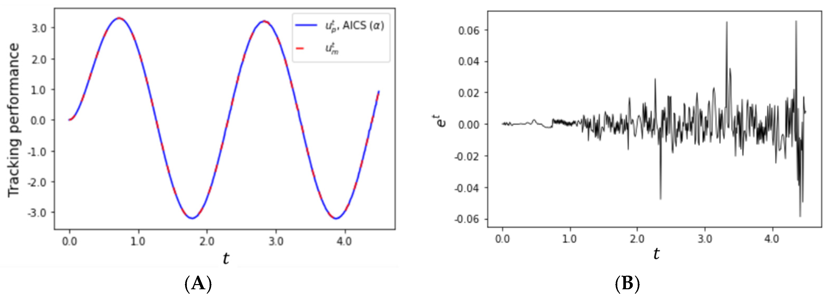
Figure 12. Controllability of the AICS designed by scenario 2. (A) Control response. (B) Tracking error.
Electronics 14 03157 g012
Figure 13. Controllability of the AICS designed by scenario 3. (A) Control response. (B) Tracking error.
Electronics 14 03157 g013
Figure 11 illustrates the control response [76] and the tracking error of the AICS designed in scenario 1. Subfigure (A) initially exhibits fluctuations in the control response, which stabilize as t progresses. The notably different shape of u t in the initial control process (see Figure 8A) may contribute to these fluctuations, suggesting that the STNNC without incorporating the HPO lacks the self-tuning capacity to mitigate them. The best control response, as shown in Figure 12 [76], is achieved in scenario 2 with 2048 model parameters only in the STNNC, using the transfer learning and optimizing α . e t exhibits fluctuations but converges to a range within one-tenth of that observed in scenario 1 . Prior to t =   3.0, as shown in Figure 6, the upper bound (see Table 1) sufficiently supports the effective optimization of α . However, after this time point, it may begin to constrain the effectiveness of the optimization, as variation in α becomes restricted within an imprecisely defined range by both bounds. Nevertheless, the findings underscore that optimizing α without adjusting the size of the given search space, combined with the transfer learning, achieves the best controllability of the AICS. In scenario 3, despite exploring the hyperparameter search space four times more extensively than in scenario 2 (see Table 1) during the GP-BO process, subfigure (A) in Figure 13 displays the noisy control response. To eliminate the outliers in e t , any solution—such as all possible STNNC-related (e.g., adding HPO options including initial samples or adjusting the architecture of the MLP) and MLTM-PINN-related strategies (e.g., increasing the activation frequency)—must require an increase in computational resources. Figure 9 and Figure 10 indicate that scenario 2 is also superior to scenario 3 in terms of the computational efficiency, with less frequent meta-learning activation and quicker adaptation in control.

5. Conclusions

We propose the AICS with a learning-while-controlling capability for the highly nonlinear SISO plant. The control system consists of two subsystems, streamlining its structure: the MLTM-PINN for plant identification and the self-tuning STNNC with high adaptability. The AICS design involves revising the MRAC framework, integrating the nonlinear controller and adaptation laws into the STNNC based on the GP-BO strategy, and upgrading the DE solver to the MLTM-PINN.
The MLTM-PINN is devised with several essential techniques. The MLTM can intelligently resolve the conflict between high controllability and control efficiency, as the triggered mechanism activates the meta-learning only when one of the error thresholds detects a deterioration in the controllability. The quick adaptation in the MLTM-PINN, expected through the transfer learning and meta-learning, is restrictive when the HPO strategies are involved with the STNNC design. The PINN, trained through self-supervised learning without the need for labelled data, facilitates the online integration of learning and control modes.
For designing the STNNC, three distinct scenarios are tested. Scenario 1 shows the poorest tracking performance, particularly in the initial control response, due to the exclusion of the HPO, although it enables f θ m ( t ) to quickly adapt to u t . Scenario 2 demonstrates that the combination of the transfer learning and the HPO in the STNNC effectively corrects the shape of u t , leading to superior controllability and the highest control efficiency. However, Scenarios 2 and 3 leave the challenge of quick adaptation in the MLTM-PINN.
The study demonstrates the feasibility for challenging real-world applications in scenario 2. Yet, it still needs the resource-intensive meta-learning-based approach. Our upcoming study will provide solutions to this issue by the use of more adaptable neural networks for each subsystem.

6. Future Study

We plan to tackle the challenge of further reducing computational resources without compromising control performance by replacing the MLP with either a liquid neural network (LNN), a transformer neural network (TNN) with a single attention mechanism, or a combination of both, with and without the meta-learning. This replacement aims to preserve the high adaptability of the PINN by leveraging the key strengths of the neural networks. For the LNN, we anticipate higher adaptability to the dynamic input evolution. This enhanced adaptability is attributed to the use of ODE-based activations, which allow both subsystems to more effectively model continuous-time dynamics under rapidly changing inputs. In the case of the TNN, the self-attention mechanism is anticipated to sustain the influence of an initial constraint throughout the entire control process. Ultimately, combining physics-informed machine learning with a TNN could globally propagate the long-range dependency between initial constraints and outputs across a long time span. In addition, fine-tuning target continuous hyperparameters using hybrid optimization is also expected to enhance the adaptability of the STNNC and mitigate the dynamic input evolution, thereby reducing the frequency of the meta-learning activations.
In the final stage of control system design, stability verification is essential to ensure that the proposed system maintains bounded behaviour over time under both nominal and perturbed conditions. We will offer a numerical framework for assessing whether the system’s states converge to a desired equilibrium point or remain within an acceptable region of attraction, using a Lyapunov function based on a partial differential equation.

Author Contributions

Conceptualization, W.K.S.; funding acquisition, M.-H.K.; investigation, W.D., W.K.S. and D.-W.L.; methodology, W.K.S.; project administration, M.-H.K.; resources, D.-W.L.; software, W.D. and S.D.; supervision, W.K.S. and M.-H.K.; validation, W.D. and W.K.S.; writing—original draft, W.D. and W.K.S.; writing—review and editing, W.K.S. All authors have read and agreed to the published version of the manuscript.

Funding

This work was funded by a grant from the National Research Foundation of Korea (NRF) supported by the Korea government (MSIT) under grant number 2021R1A2C2006025. The APC was funded by the NRF grant.

Data Availability Statement

Dataset available on request from the authors.

Acknowledgments

The authors gratefully acknowledge the financial support provided by the National Research Foundation of Korea (NRF) and the Korea government (MSIT) through grant number 2021R1A2C2006025.

Conflicts of Interest

The authors declare no conflicts of interest. The funders had no role in the design of the study; in the collection, analyses, or interpretation of data; in the writing of the manuscript; or in the decision to publish the results.

References

  1. Duanyai, W.; Song, W.K.; Konghuayrob, P.; Parnichkun, M. Event-triggered model reference adaptive control system design for SISO plants using meta-learning-based physics-informed neural networks without labeled data and transfer learning. Int. J. Adapt. Control Signal Process. 2024, 38, 1442–1456. [Google Scholar] [CrossRef]
  2. Antsaklis, P.J. Intelligent Control. Wiley Encyclopedia of Electrical and Electronics Engineering; John Wiley & Sons, Inc.: Hoboken, NJ, USA, 1999; pp. 493–505. [Google Scholar]
  3. Jagannathan, S.; Lewis, F.L.T. Identification of nonlinear dynamical systems using multilayered neural networks. Automatica 1996, 32, 1707–1712. [Google Scholar] [CrossRef]
  4. Kwan, C.M.; Lewis, F.L.; Dawson, D.M. Robust neural-network control of rigid-link electrically driven robots. IEEE Trans. Neural Netw. 1998, 9, 581–588. [Google Scholar] [CrossRef] [PubMed]
  5. Lewis, F.L.; Liu, K.; Yesildirek, A. Neural net robot controller with guaranteed tracking performance. IEEE Trans. Neural Netw. 1995, 6, 703–715. [Google Scholar] [CrossRef] [PubMed]
  6. Lewis, F.L.; Yesildirek, A.; Kai, L. Multilayer neural-net robot controller with guaranteed tracking performance. IEEE Trans. Neural Netw. 1996, 7, 388–399. [Google Scholar] [CrossRef]
  7. Yeşildirek, A.; Lewis, F.L. Feedback linearization using neural networks. Automatica 1995, 31, 1659–1664. [Google Scholar] [CrossRef]
  8. Yu, S.-H.; Annaswamy, A.M. Stable neural controllers for nonlinear dynamic systems. Automatica 1998, 34, 641–650. [Google Scholar] [CrossRef]
  9. Gu, F.; Yin, H.; Ghaoui, L.E.; Arcak, M.; Seiler, P.J.; Jin, M. Recurrent Neural Network Controllers Synthesis with Stability Guarantees for Partially Observed Systems; Association for the Advancement of Artificial Intelligence (AAAI): Washington, DC, USA, 2022; pp. 5385–5394. [Google Scholar]
  10. Widrow, B.; Walach, E. Adaptive Inverse Control: A Signal Processing Approach; Wiley-IEEE Press: Hoboken, NJ, USA, 2007. [Google Scholar]
  11. Nahas, E.P.; Henson, M.A.; Seborg, D.E. Nonlinear internal model control strategy for neural network models. Comput. Chem. Eng. 1992, 16, 1039–1057. [Google Scholar] [CrossRef]
  12. Hunt, K.J.; Sbarbaro, D.; Żbikowski, R.; Gawthrop, P.J. Neural networks for control systems—A survey. Automatica 1992, 28, 1083–1112. [Google Scholar] [CrossRef]
  13. Narendra, K.S.; Parthasarathy, K. Identification and control of dynamical systems using neural networks. IEEE Trans. Neural Netw. 1990, 1, 4–27. [Google Scholar] [CrossRef]
  14. Wang, D.; Liu, D.; Zhang, Q.; Zhao, D. Data-based adaptive critic designs for nonlinear robust optimal control with uncertain dynamics. IEEE Trans. Syst. Man Cybern. Syst. 2016, 46, 1544–1555. [Google Scholar] [CrossRef]
  15. Jin, L.; Nikiforuk, P.N.; Gupta, M.M. Direct adaptive output tracking control using multilayered neural networks. J. Eng. Technol. 1993, 140, 393–398. [Google Scholar] [CrossRef]
  16. Jin, L.; Nikiforuk, P.N.; Gupta, M.M. Fast neural learning and control of discrete-time nonlinear systems. IEEE Trans. Syst. Man Cybern. 1995, 25, 478–488. [Google Scholar] [CrossRef]
  17. Levin, A.U.; Narenda, K.S. Control of nonlinear dynamical systems using neural networks. II. Observability, identification, and control. IEEE Trans. Neural Netw. 1996, 7, 40–42. [Google Scholar] [CrossRef]
  18. Sutton, R.S.; Barto, A.G. Reinforcement Learning, an Introduction, 2nd ed.; The MIT Press: Cambridge, MA, USA, 1998. [Google Scholar]
  19. Kaelbling, L.P.; Littman, M.L.; Moore, A.W. Reinforcement learning: A survey. J. Artif. Intell. Res. 1996, 4, 237–285. [Google Scholar] [CrossRef]
  20. Shen, Y.; Tobia, M.J.; Sommer, T.; Obermayer, K. Risk-sensitive reinforcement learning. Neural Comput 2014, 26, 1298–1328. [Google Scholar] [CrossRef]
  21. Chen, H.; Liu, C. Safe and sample-efficient reinforcement learning for clustered dynamic environments. IEEE Control Syst. Lett. 2022, 6, 1928–1933. [Google Scholar] [CrossRef]
  22. Cheng, Y.; Zhao, P.; Hovakimyan, N. Safe and efficient reinforcement learning using disturbance-observer-based control barrier functions. In Proceedings of the 5th Annual Learning for Dynamics and Control Conference, Philadelphia, PA, USA, 14–16 June 2023; PMLR 211: New York, NY, USA, 2023; pp. 104–115. Available online: https://proceedings.mlr.press/v211/cheng23a.html (accessed on 3 August 2025).
  23. Wachi, A.; Hashimoto, W.; Shen, X.; Hashimoto, K. Safe exploration in reinforcement learning: A generalized formulation and algorithms. In Proceedings of the 37th International Conference on Neural Information Processing Systems, New Orleans, LA, USA; 2024. [Google Scholar]
  24. Du, H.; Hao, B.; Zhao, J.; Zhang, J.; Wang, Q.; Yuan, Q. A path planning approach for mobile robots using short and safe Q-learning. PLoS ONE 2022, 17, e0275100. [Google Scholar] [CrossRef]
  25. Xu, H.; Zhan, X.; Zhu, X. Constraints Penalized Q-Learning for Safe Offline Reinforcement Learning; Association for the Advancement of Artificial Intelligence (AAAI): Washington, DC, USA, 2022; pp. 8753–8760. [Google Scholar]
  26. Ge, Y.; Zhu, F.; Ling, X.; Liu, Q. Safe Q-learning method based on constrained markov decision processes. IEEE Access 2019, 7, 165007–165017. [Google Scholar] [CrossRef]
  27. Raissi, M.; Perdikaris, P.; Karniadakis, G.E. Physics-informed neural networks: A deep learning framework for solving forward and inverse problems involving nonlinear partial differential equations. J. Comput. Phys. 2019, 378, 686–707. [Google Scholar] [CrossRef]
  28. Dong, S.; Li, Z. Local extreme learning machines and domain decomposition for solving linear and nonlinear partial differential equations. Comput. Methods Appl. Mech. Eng. 2021, 387, 114129. [Google Scholar] [CrossRef]
  29. Jagtap, A.D.; Kharazmi, E.; Karniadakis, G.E. Conservative physics-informed neural networks on discrete domains for conservation laws: Applications to forward and inverse problems. Comput. Methods Appl. Mech. Eng. 2020, 365, 113028. [Google Scholar] [CrossRef]
  30. Zhang, R.; Liu, Y.; Sun, H. Physics-guided convolutional neural network (PhyCNN) for data-driven seismic response modeling. Eng. Struct. 2020, 215, 110704. [Google Scholar] [CrossRef]
  31. Zhu, Y.; Zabaras, N.; Koutsourelakis, P.-S.; Perdikaris, P. Physics-constrained deep learning for high-dimensional surrogate modeling and uncertainty quantification without labeled data. J. Comput. Phys. 2019, 394, 56–81. [Google Scholar] [CrossRef]
  32. Sun, L.; Wang, J.-X. Physics-constrained bayesian neural network for fluid flow reconstruction with sparse and noisy data. Theor. Appl. Mech. Lett. 2020, 10, 161–169. [Google Scholar] [CrossRef]
  33. Ma, Y.; Xu, X.; Yan, S.; Ren, Z. A Preliminary study on the resolution of electro-thermal multi-physics coupling problem using physics-informed neural network (PINN). Algorithms 2022, 15, 53. [Google Scholar] [CrossRef]
  34. Amini Niaki, S.; Haghighat, E.; Campbell, T.; Poursartip, A.; Vaziri, R. Physics-informed neural network for modelling the thermochemical curing process of composite-tool systems during manufacture. Comput. Methods Appl. Mech. Eng. 2021, 384, 113959. [Google Scholar] [CrossRef]
  35. Robinson, H.; Pawar, S.; Rasheed, A.; San, O. Physics guided neural networks for modelling of non-linear dynamics. Neural Netw. 2022, 154, 333–345. [Google Scholar] [CrossRef]
  36. Hochreiter, S.; Younger, A.S.; Conwell, P.R. Learning to learn using gradient descent. In Proceeding of the Artificial Neural Networks-ICANN 2001, Vienna, Austria, 21–25 August 2001. [Google Scholar]
  37. Younger, A.S.; Hochreiter, S.; Conwell, P.R. Meta-Learning with Backpropagation; IEEE: Washington, DC, USA, 2001; pp. 2001–2006. [Google Scholar]
  38. Finn, C.; Abbeel, P.; Levine, S. Model-agnostic meta-learning for fast adaptation of deep networks. In Proceedings of the 34th International Conference on Machine Learning, Sydney, NSW, Australia, 6–11 August 2017. [Google Scholar]
  39. Liu, X.; Zhang, X.; Peng, W.; Zhou, W.; Yao, W. A novel meta-learning initialization method for physics-informed neural networks. Neural Comput. Appl. 2022, 34, 14511–14534. [Google Scholar] [CrossRef]
  40. Psaros, A.F.; Kawaguchi, K.; Karniadakis, G.E. Meta-learning PINN loss functions. J. Comput. Phys. 2022, 458, 111121. [Google Scholar] [CrossRef]
  41. Penwarden, M.; Zhe, S.; Narayan, A.; Kirby, R.M. A metalearning approach for Physics-informed neural networks (PINNs): Application to parameterized PDEs. J. Comput. Phys. 2023, 477, 111912. [Google Scholar] [CrossRef]
  42. Nicodemus, J.; Kneifl, J.; Fehr, J.; Unger, B. Physics-informed neural networks-based model predictive control for multi-link manipulators. IFAC-PapersOnline 2022, 55, 331–336. [Google Scholar] [CrossRef]
  43. Gokhale, G.; Claessens, B.; Develder, C. Physics informed neural networks for control oriented thermal modeling of buildings. Appl. Energy 2022, 314, 118852. [Google Scholar] [CrossRef]
  44. García-Cervera, C.J.; Kessler, M.; Periago, F. Control of partial differential equations via physics-informed neural networks. J. Optim. Theory Appl. 2022, 196, 391–414. [Google Scholar] [CrossRef]
  45. Shi, G.; Azizzadenesheli, K.; O’Connell, M.; Chung, S.-J.; Yue, Y. Meta-adaptive nonlinear control: Theory and algorithms. In Proceedings of the 35th International Conference on Neural Information Processing Systems 34, Vancouver, BC, Canada, 6–14 December 2021; Available online: https://proceedings.neurips.cc/paper_files/paper/2021/hash/52fc2aee802efbad698503d28ebd3a1f-Abstract.html (accessed on 3 August 2025).
  46. Richards, S.M.; Azizan, N.; Slotine, J.-J.; Pavone, M. Adaptive-control-oriented meta-learning for nonlinear systems. Robotics: Science and Systems. arXiv 2021, arXiv:2103.04490. [Google Scholar] [CrossRef]
  47. Nagabandi, A.; Clavera, I.; Liu, S.; Fearing, R.S.; Abbeel, P.; Levine, S.; Finn, C. Learning to Adapt in Dynamic, Real-World Environments through Meta-Reinforcement Learning. In Proceedings of the 2nd Workshop on Meta-Learning, Montreal, QC, Canada, 8 December 2018. [Google Scholar] [CrossRef]
  48. Belkhale, S.; Li, R.; Kahn, G.; McAllister, R.; Calandra, R.; Levine, S. Model-based meta-reinforcement learning for flight with suspended payloads. IEEE Robot. Autom. Lett. 2021, 6, 1471–1478. [Google Scholar] [CrossRef]
  49. Penwarden, M.; Jagtap, A.D.; Zhe, S.; Karniadakis, G.E.; Kirby, R.M. A unified scalable framework for causal sweeping strategies for physics-informed neural networks (PINNs) and their temporal decompositions. J. Comput. Phys. 2023, 493, 112464. [Google Scholar] [CrossRef]
  50. Masood, A. Automated Machine Learning: Hyperparameter Optimization, Neural Architecture Search, and Algorithm Selection with Cloud Platforms; Packt Publishing Limited: Birmingham, UK, 2023. [Google Scholar]
  51. Kushner, H.J. A new method of locating the maximum point of an arbitrary multipeak curve in the presence of noise. J. Fluids Eng. 1964, 86, 97–106. [Google Scholar] [CrossRef]
  52. Zhilinskas, A.G. Single-step Bayesian search method for an extremum of functions of a single variable. J. Cybermetics Syst. Anal. 1975, 11, 160–166. [Google Scholar] [CrossRef]
  53. Močkus, J. On Bayesian Methods for Seeking the Extremum; Springer: Berlin/Heidelberg, Germany, 1975; pp. 400–404. [Google Scholar]
  54. Jones, D.R.; Schonlau, M.; Welch, W.J. Efficient global optimization of expensive black-box functions. J. Glob. Optim. 1998, 13, 455–492. [Google Scholar] [CrossRef]
  55. Snoek, J.; Larochelle, H.; Adams, R.P. Practical bayesian optimization of machine learning algorithms. In Proceedings of the Advances in Neural Information Processing Systems 25, Lake Tahoe, NV, USA, 3–6 December 2012; Available online: https://proceedings.neurips.cc/paper/2012/hash/05311655a15b75fab86956663e1819cd-Abstract.html (accessed on 3 August 2025).
  56. Salemi, P.; Nelson, B.L.; Staum, J. Discrete Optimization via Simulation Using Gaussian Markov Random Fields; IEEE: Georgia, GA, USA, 2014; pp. 3809–3820. [Google Scholar]
  57. Mehdad, E.; Kleijnen, J.P.C. Efficient global optimisation for black-box simulation via sequential intrinsic Kriging. J. Oper. Res. Soc. 2018, 69, 1725–1737. [Google Scholar] [CrossRef]
  58. Booker, A.J.; Dennis, J.J.E.; Frank, P.D.; Serafini, D.B.; Torczon, V.; Trosset, M.W. A rigorous framework for optimization of expensive functions by surrogates. J. Struct. Multidiscip. Optim. 1999, 17, 1–13. [Google Scholar] [CrossRef]
  59. Regis, R.G.; Shoemaker, C.A. Constrained global optimization of expensive black box functions using radial basis functions. J. Glob. Optim. 2016, 31, 153–171. [Google Scholar] [CrossRef]
  60. Regis, R.G.; Shoemaker, C.A. Improved strategies for radial basis function methods for global optimization. J. Glob. Optim. 2006, 37, 113–135. [Google Scholar] [CrossRef]
  61. Regis, R.G.; Shoemaker, C.A. Parallel radial basis function methods for the global optimization of expensive functions. Eur. J. Oper. Res. 2007, 182, 514–535. [Google Scholar] [CrossRef]
  62. Audet, C.; Denni, J.; Moore, D.; Booker, A.; Frank, P. A surrogate-model-based method for constrained optimization. In Proceedings of the 8th Symposium on Multidisciplinary Analysis and Optimization, Long Beach, CA, USA, 6–8 September 2000. [Google Scholar]
  63. Mahendran, N.; Wang, Z.; Hamze, F.; Freitas, N.D. Adaptive MCMC with Bayesian optimization. In Proceedings of the Fifteenth International Conference on Artificial Intelligence and Statistics, Proceedings of Machine Learning Research; Canary Island, Spain, 21–23 April 2021, Available online: https://proceedings.mlr.press/v22/mahendran12.html (accessed on 3 August 2025).
  64. Meeds, E.; Welling, M. GPS-ABC: Gaussian process surrogate approximate Bayesian computation. In Proceedings of the Thirtieth Conference on Uncertainty in Artificial Intelligence, Quebec City, QC, Canada, 23–27 July 2014. [Google Scholar]
  65. Genton, M.G. Classes of kernels for machine learning: A statistics perspective. J. Mach. Learn. Res. 2001, 2, 299–312. [Google Scholar]
  66. Sollich, P.; Urry, M.; Coti, C. Kernels and learning curves for Gaussian process regression on random graphs. In Proceedings of the Advances in Neural Information Processing Systems 22, Vancouver, BC, Canada, 7–10 December 2009; Available online: https://proceedings.neurips.cc/paper/2009/hash/92cc227532d17e56e07902b254dfad10-Abstract.html (accessed on 3 August 2025).
  67. Wilson, A.; Adams, R. Gaussian Process Kernels for Pattern Discovery and Extrapolation. In Proceedings of the 30th International Conference on Machine Learning, Atlanta, GA, USA, 16–21 June 2021; PMLR: New York, NY, USA, 2013; Volume 28, pp. 1067–1075. Available online: https://proceedings.mlr.press/v28/wilson13.html (accessed on 3 August 2025).
  68. Duvenaud, D.; Lloyd, J.; Grosse, R.; Tenenbaum, J.; Zoubin, G. Structure discovery in nonparametric regression through compositional kernel search. In Proceedings of the 30th International Conference on Machine Learning, Proceedings of Machine Learning Research; Atlanta, GA, USA, 16–21 June 2023, Available online: https://proceedings.mlr.press/v28/duvenaud13.html (accessed on 3 August 2025).
  69. Roman, I.; Santana, R.; Mendiburu, A.; Lozano, J.A. An experimental study in adaptive kernel selection for Bayesian optimization. IEEE Access 2019, 7, 184294–184302. [Google Scholar] [CrossRef]
  70. Couckuyt, I.; Deschrijver, D.; Dhaene, T. Fast calculation of multiobjective probability of improvement and expected improvement criteria for Pareto optimization. J. Glob. Optim. 2013, 60, 575–594. [Google Scholar] [CrossRef]
  71. Chapelle, O.; Li, L. An Empirical Evaluation of Thompson Sampling. Curran Associates. In Proceedings of the Advances in Neural Information Processing Systems 24, Granada, Spain, 12–17 December 2011; Available online: https://proceedings.neurips.cc/paper/2011/hash/e53a0a2978c28872a4505bdb51db06dc-Abstract.html (accessed on 3 August 2025).
  72. Duanyai, W.; Song, W.K.; Chitthamlerd, T.; Kumar, G. Meta-learning-based physics-informed neural network: Numerical simulations of initial value problems of nonlinear dynamical systems without labeled data and correlation analyses. J. Nonlinear Model. Anal. 2024, 6, 485–513. [Google Scholar] [CrossRef]
  73. Nocedal, J. Updating quasi-Newton matrices with limited storage. Math. Comput. 1980, 35, 773–782. [Google Scholar] [CrossRef]
  74. Byrd, R.H.; Nocedal, J.; Schnabel, R.B. Representations of quasi-Newton matrices and their use in limited memory methods. Math. Program. 1994, 63, 129–156. [Google Scholar] [CrossRef]
  75. Liu, D.C.; Nocedal, J. On the limited memory BFGS method for large scale optimization. Math. Program. 1989, 45, 503–528. [Google Scholar] [CrossRef]
  76. Duanyai, W. A Comparision of the Controllability of Model Reference Adaptive Control and Intelligent Control Systems for a Nonlinear SISO Plant; King Mongkut Institute of Technology Ladkrabang: Bangkok, Thailand, 2024. [Google Scholar]
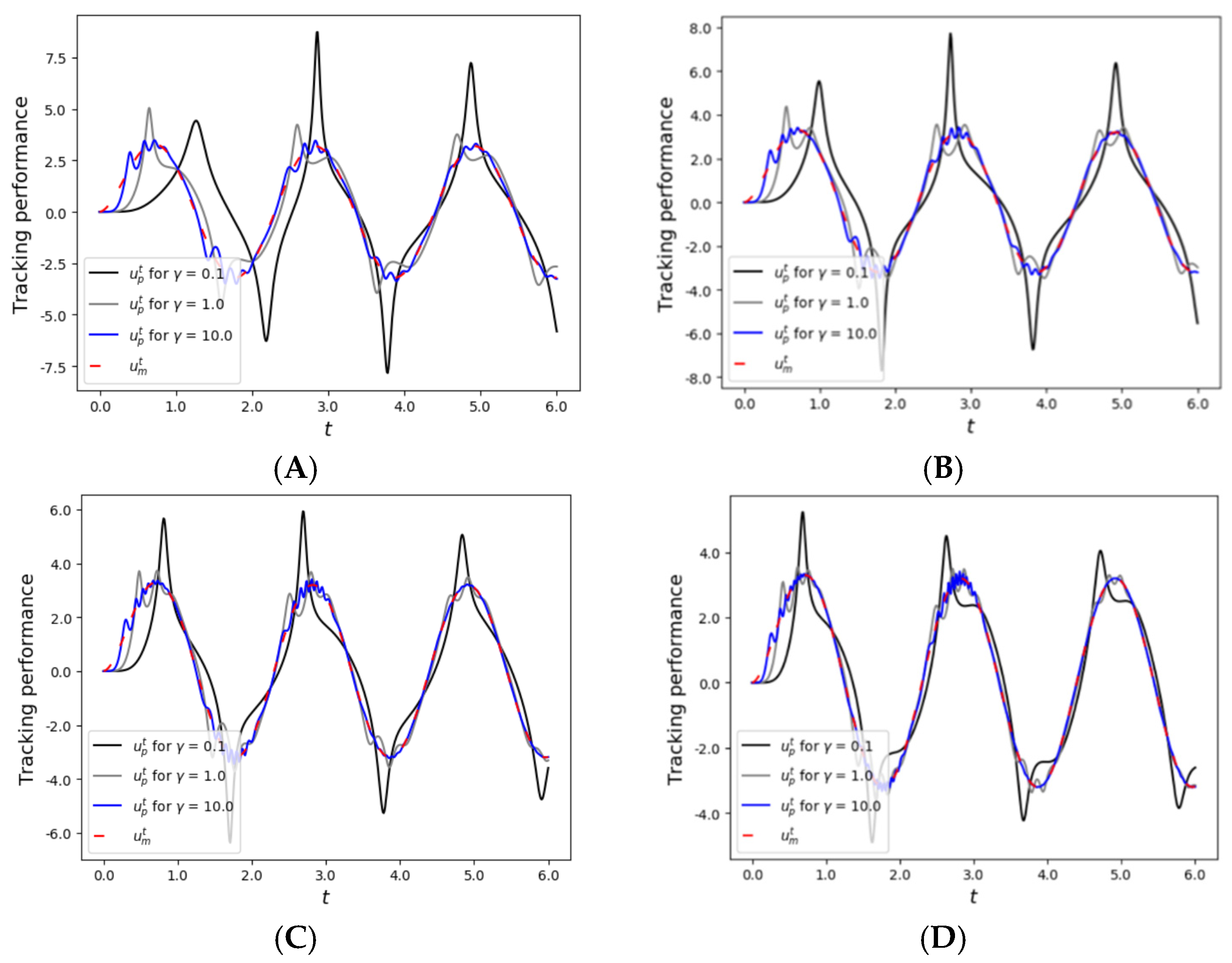
Figure 2. Controllability of the MRAC system for varying γ and B p . (A) Control responses at B p   = 1.5. (B) Control responses at B p   = 3.0. (C) Control responses at B p   = 6.0. (D) Control responses at B p   = 12.0.
Electronics 14 03157 g002
Figure 3. A subsequent process of control response divergence at B p = 3.0. (A) Initial phase of control response divergence at γ = 71.0. (B) Control response divergence at γ = 72.0.
Electronics 14 03157 g003
Figure 4. Architecture of the PINN with an MLP and a module integrating physics laws.
Electronics 14 03157 g004
Figure 6. Change in the optimal value of α over t in scenario 2.
Electronics 14 03157 g006
Figure 7. Changes in the optimal values of the target hyperparameters over t in scenario 3. (A) Change in the optimal value of α . (B) Change in the optimal number of NE in the first hidden layer. (C) Change in the optimal number of NE in the second hidden layer.
Electronics 14 03157 g007
Figure 8. Changes in u t over t in the scenarios. (A) Scenario 1. (B) Scenario 2. (C) Scenario 3.
Electronics 14 03157 g008
Figure 9. Scenarios with distinct triggering event profiles. (A) Scenario 1 with 49 activations. (B) Scenario 2 with 34 activations. (C) Scenario 3 with 40 activations.
Electronics 14 03157 g009
Table 1. HPO configurations for the scenarios.
MTRTarget Hyperparameters
α NE (First Hidden Layer)NE (Second Hidden Layer)
Min. VInt. VMax. VMin. VInt. VMax. VMin. VInt. VMax. V
Scenario 1 0.018256
Scenario 250.0010.0010.028256
Scenario 3200.0010.0010.028256204882562048
MTR denotes the maximum number of trials for the HPO at each t . Min. V, Int. V, and Max. V denote, respectively, the lower bound value, the initial value, and the upper bound value of each target hyperparameter search space.
Disclaimer/Publisher’s Note: The statements, opinions and data contained in all publications are solely those of the individual author(s) and contributor(s) and not of MDPI and/or the editor(s). MDPI and/or the editor(s) disclaim responsibility for any injury to people or property resulting from any ideas, methods, instructions or products referred to in the content.