Article

Laser Radar and Micro-Light Polarization Image Matching and Fusion Research

Shijiazhuang Campus, Army Engineering University, Shijiazhuang 050003, China
*
Author to whom correspondence should be addressed.
Electronics 2025, 14(15), 3136; https://doi.org/10.3390/electronics14153136
Submission received: 8 July 2025 / Revised: 2 August 2025 / Accepted: 4 August 2025 / Published: 6 August 2025
(This article belongs to the Special Issue Image and Signal Processing Techniques and Applications)

Abstract

Aiming at addressing the defect of the data blindness of a LiDAR point cloud in transparent media such as glass in low illumination environments, a new method is proposed to realize covert target reconnaissance, identification and ranging using the fusion of a shimmering polarized image and a laser LiDAR point cloud, and the corresponding system is constructed. Based on the extraction of pixel coordinates from the 3D LiDAR point cloud, the method adds information on the polarization degree and polarization angle of the micro-light polarization image, as well as on the reflective intensity of each point of the LiDAR. The mapping matrix of the radar point cloud to the pixel coordinates is made to contain depth offset information and show better fitting, thus optimizing the 3D point cloud converted from the micro-light polarization image. On this basis, algorithms such as 3D point cloud fusion and pseudo-color mapping are used to further optimize the matching and fusion procedures for the micro-light polarization image and the radar point cloud, so as to successfully realize the alignment and fusion of the 2D micro-light polarization image and the 3D LiDAR point cloud. The experimental results show that the alignment rate between the 2D micro-light polarization image and the 3D LiDAR point cloud reaches 74.82%, which can effectively detect the target hidden behind the glass under the low illumination condition and fill the blind area of the LiDAR point cloud data acquisition. This study verifies the feasibility and advantages of “polarization + LiDAR” fusion in low-light glass scene reconnaissance, and it provides a new technological means of covert target detection in complex environments.

1. Introduction

Night vision imaging technology is similar to normal imaging technology in that it involves imaging received targets and scenes through a detector. However, night vision imaging techniques have a more challenging low-light operating environment, resulting in relatively poor image quality. On the other hand, the micro-light imaging technique utilizes the weak nighttime light reflected from the target object to perform imaging, with the resulting images usually having low contrast and requiring further processing [1]. With the gradual recognition and utilization of polarized imaging properties, polarization imaging technology was introduced into night vision imaging technology, which resulted in night vision polarization imaging technology [2]. Polarization imaging technology can not only obtain information from traditional images but also obtain the polarization information of the target scene on that basis. Polarization information enhances the contour information and detailed texture of an object, thus improving the contrast between the target and the scene. In addition, information such as the texture, material, and surface roughness of the target object will be reflected in polarization images in different ways. However, micro-light polarization images can only provide two-dimensional planar information, and the spatial position and depth perception of the target object are weak.
In recent years, LiDAR has been widely used in many fields [3,4,5]. LiDAR has the advantages of strong 3D perception, high measurement accuracy, and strong immunity against interference, which are unrivaled by other imaging technologies [6]. With the continuous advancement of laser and electronic technologies, significant breakthroughs have been made in laser radar imaging technology. Various new types of LiDAR systems have emerged, such as scanning LiDAR and imaging LiDAR [7]. Scanning LiDAR scans across the target area mechanically or optically to obtain 2D or 3D information about the target [8]. Imaging LiDAR adopts more advanced detectors and signal processing techniques to directly acquire target image information, and its imaging resolution and accuracy have been significantly improved. Since then, the fusion of LiDAR and 2D images has been explored [9]. Hans Moravec (Carnegie Mellon University) conducted early research in the field of robotic navigation and proposed a sensor-based approach to environmental awareness [10]. However, LiDAR point cloud data lacks detailed features such as the surface texture and material of the target object. Paul Besl and Neil McKay proposed the iterative closest point (ICP) algorithm, which laid the foundation for point cloud alignment [11]. In 2005, Sebastian Thrun, the “father of driverlessness”, led the team that developed an autonomous driving system based on LiDAR and camera fusion. In 2012, Andreas Geiger (creator of the KITTI dataset) released the KITTI dataset, which pushed forward the algorithm for the fusion of LiDAR and image research [12,13]. Wei Kai has achieved remarkable results in terms of laser phased array technology and multi-band image matching and fusion technology [14]. Zhiyan Dong (Fudan University) made a breakthrough in relation to the SLAM map-building method for the fusion of LiDAR and binocular vision during UAV level flight [15]. Youth Zhang (Huaiyin Institute of Technology) developed an intelligent mobile robot system based on the ROS platform, which realized the efficient fusion of camera and LiDAR [16]. In 2017, Charles Qi (Stanford University) proposed PointNet, which is the first application of deep learning in point cloud data processing [17].
Although the above fusion methods can improve the comprehensive information available to optical measurement systems [18], they cannot effectively enhance the description of tail features such as the surface texture and material of target objects through point cloud data. In 2024, Li M and team pointed out that the polarization intensity can serve as an additional characteristic channel for geometric completion [19]. In 2024, Liu H proposed the fusion of the visible light polarized texture and a portable LiDAR point cloud, which can achieve millimeter-level defect detection of wooden components, verifying the advantages of polarization LiDAR fusion in weak texture structures [20]. In 2024, Dong Q et al. used visible light polarization images to assist with LiDAR point cloud denoising and surface detail restoration in the reconstruction of ancient rockeries, proving that polarization information can effectively improve the reconstruction integrity of complex geometries [21]. In 2024, Zhu Q pointed out that strategies based on the polarization degree, such as point cloud color transfer and geometric consistency checking, can be directly used to improve the quality of training samples in low-light scenes [22]. Although there is a lot of literature on image fusion with LiDAR point clouds [23,24,25,26], no studies have been reported on the use of micro-light polarization images to compensate for the blind spots of LiDAR point cloud data. The aim of this study is to construct a micro-light polarization and LiDAR acquisition system to collect and process data from different sensors, fully exploit the advantages of each sensor, and compensate for their respective shortcomings, so as to obtain more comprehensive, accurate, and reliable target information. To this end, an optimal scheme for matching and fusing micro-light polarization images with radar point cloud data is proposed.
This paper first elaborates on the principle and optimization algorithm for matching and fusing LiDAR with low-light polarization images. Then, the construction methods for the low-light polarization imaging system and the LiDAR point cloud acquisition system, along with related image processing techniques, are introduced. Finally, using the optimized matching–fusion algorithm, two-dimensional low-light polarization images and LiDAR point clouds are fused and optimized, filling the blind spots in LiDAR data acquisition in low-light environments.

2. Preliminary

2.1. Matching of LiDAR and Low-Light Polarization Images

Because of the strong laser reflection by glass, LiDAR can acquire point clouds in ordinary scenes but fails to detect targets behind optical glass. Therefore, the position of the glass surface is first derived from the LiDAR point cloud. Then, micro-light polarization images of the same scene are acquired. A MATLAB program is used to process these images to generate micro-light polarization images [23]. The LiDAR point cloud is a three-dimensional image, while the microlight polarization image is a two-dimensional image. Thus, the matching–fusion of the LiDAR and micro-light polarization image is the matching–fusion of three-dimensional point cloud and two-dimensional image.
Image matching involves co-calibrating the LiDAR camera coordinate system, extracting and matching feature points, and establishing correspondences between them. For LiDAR and camera systems, the same target is targeted within a common field of view due to the fact that the LiDAR resolution is lower than the camera resolution. Therefore, each 3D point cloud has a unique image pixel point corresponding to it. In other words, the external parameter calibration of the LiDAR and camera system can be understood as solving the mapping matrix between the 3D LiDAR point cloud and the image pixel points. First, the camera’s intrinsic matrix is obtained. Next, the corresponding feature point coordinates are extracted from both the LiDAR point cloud and the optical image, and the extrinsic calibration is formulated as a perspective-n-point (PnP) problem to compute the mapping matrix.
After obtaining the feature points corresponding to the LiDAR and 2D images, the coordinates of the feature points are (XL, YL, ZL) in the LiDAR coordinate system, and (u, v) in the pixel coordinate system; their relationship is established as follows:
u v 1 = K R T 0 1 X L Y L Z L 1 = M X L Y L Z L 1 = m 11 m 12 m 13 m 14 m 21 m 22 m 23 m 24 m 31 m 32 m 33 m 34
where K denotes the camera internal reference; R denotes the rotation matrix from the LiDAR coordinate system to the camera coordinate system; and T denotes the translation vector. By extracting a number of sets of LiDAR and image corresponding feature points, a system of constraint equations is established to be solved for the 12 elements in the matrix M. Expanding Equation (1), we get
u = m 11 X L + m 12 Y L + m 13 Z L + m 14 v = m 21 X L + m 22 Y L + m 23 Z L + m 24 1 = m 31 X L + m 32 Y L + m 33 Z L + m 34
At least six sets of feature points are required. In practice, additional feature points are collected to reduce the errors. The mapping matrix is first initialized via the least squares method and then refined to obtain the final result.
When the mapping matrix M is solved by the least squares method, errors may arise in both the localization and the depth of the feature points. This stems from the mismatch between the pixel-level positioning error of low-light polarization images and that of LiDAR point clouds after projection. Consequently, the per-point error increases and is further amplified by the distance. In response to the above errors, this article first uses the least squares method to assign weights wi = 1/(σi2) to each pair of feature points, and then weights the residuals twice to further reduce the average error.

2.2. Fusion Algorithm of LiDAR and Micro-Light Polarization Images

The fusion of point cloud and image is based on the premise of the alignment of the two, through the alignment of the point cloud and image data, to establish the correspondence between each 3D point and its corresponding image pixel. First, the 3D point cloud is projected onto the optical image to obtain the corresponding pixel coordinates (x, y). Then, the R, G, B values at pixel (x, y) are assigned to the point cloud, thereby coloring the 3D data with true-color texture. After obtaining the optimized extrinsic matrix, the relationship between image and point cloud coordinates is established via the covariance equation, and the R, G, B values of each image pixel are transferred to the corresponding point in the point cloud model, completing the fusion [27].
x x 0 = f a 1 X L X C + b 1 Y L Y C + c 1 Z L Z C a 3 X L X C + b 3 Y L Y C + c 3 Z L Z C y y 0 = f a 2 X L X C + b 2 Y L Y C + c 2 Z L Z C a 3 X L X C + b 3 Y L Y C + c 3 Z L Z C
where (x, y) are the pixel coordinates corresponding to the point cloud (XL, YL, ZL) in the image plane coordinate system; (XC, YC, ZC) are the center coordinates of the camera in the image space coordinate system; f is the focal length; and (a1, a2, a3, b1, b2, b3, c1, c2, c3) are the coefficients of the rotation matrix. The corresponding R, G, B color values at (x, y) are assigned to the corresponding point cloud data using Equation (3). The fused point cloud data has the color texture information of the optical image.

2.3. Optimization of Fusion Between LiDAR and Low-Light Polarization Images

To further improve the fusion of LiDAR and low-light polarization images, the system’s feature extraction algorithm has been optimized.
Firstly, calculate the pixel coordinates of each laser point cloud, such as the pixel coordinates of the i-th laser point cloud (ui, vi).
Then, based on the 4 time-division low-light polarization images, calculate the polarization degree (DoP) and polarization angle (AoP) of each point cloud at the pixel coordinates:
DoPi = DoP[vi, ui]
AoPi = AoP[vi, ui]
Next, extract the reflection intensity Ii of each point cloud in each LiDAR point cloud datum.
Furthermore, by searching for the reflection intensity of each point cloud point and the corresponding pixel polarization degree and polarization angle information on the polarization image, a 3D feature vector combining the polarization intensity is constructed for each LiDAR point:
f i = D o P i A o P i I i
In this way, each three-dimensional laser point (Xi, Yi, Zi) is associated with its corresponding DoPi (polarization degree), AoPi (polarization angle), and echo intensity Ii on the polarization image, forming a seven-dimensional joint feature vector for all the cross-modal information of each laser point by point [28,29]:
F X Y Z = X i Y i Z i D O P i A O P i I i 1 = M p o l a r X i Y i Z i 1
Among them, the first three dimensions are the 3D coordinates of the LiDAR point; the fourth and fifth dimensions represent the degree and angle of polarization of the corresponding pixel; the sixth dimension holds the LiDAR echo intensity; and the seventh dimension is set to one for the subsequent least squares or homogeneous transformations. Simply put, the F-matrix jointly represents “3D LiDAR points + polarization features”, thereby injecting polarization information into the existing point cloud. Using the F-matrix M p o l a r and least squares method to calculate the mapping matrix in Formula (7). This mapping matrix contains depth shifts related to polarization information. By substituting M p o l a r into Formula (1) and performing the inverse operation, the low-light polarization image can be converted into a 3D point cloud without laser point cloud positions. Finally, coordinate matching and fusion are performed between the LiDAR point cloud and the low-light polarization image point cloud, and Canny’s edge detection is used for correction.
On the basis of extracting pixel coordinates, this optimization algorithm adds the extraction of vectors such as the polarization degree and polarization angle of polarized image pixels, as well as the extraction of the reflection intensity of laser radar point clouds, which improves the fitting of the mapping matrix and effectively improves the fusion effect.

3. The Proposed Fusion System

3.1. Imaging System Design and Construction

3.1.1. Micro-Light Polarization Imaging System

This research focuses on the polarization of static objects in low-light environments, so a time-sequential polarization imaging system is employed. Compared with real-time systems, the time-sequential system offers lower cost and simpler operation. In the time-sequential setup, the polarizer is rotated manually or by a motor in front of the imaging system. When the polarizer is rotated continuously, the detector obtains all the polarized components of the scene light wave through light intensity changes. Mainly based on the selection of experimental instruments to meet the system design requirements for imaging, the specific hardware is as follows:
(1) Micro-light camera: This experiment used the Watec Corporation WAT-902H2 black and white camera, as shown in Figure 1, and Table 1 shows the parameters. In the low illumination range, with the imaging lens, a clear image can be obtained.
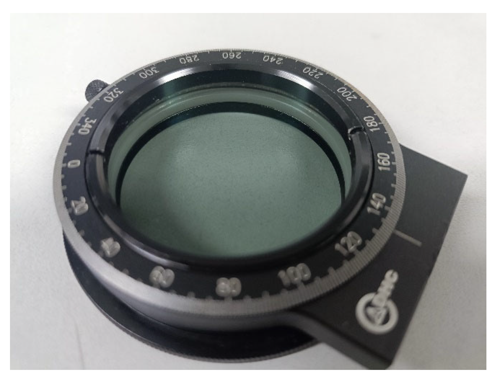
(2) Polarizer: Through early-stage comparative experiments on low-light polarization images across various bands, it was found that a polarizer film with high transmittance in the 400–1000 nm range yields the best low-light polarization imaging performance. Consequently, a polarizer with appropriate filtering properties was selected, as shown in Figure 2.
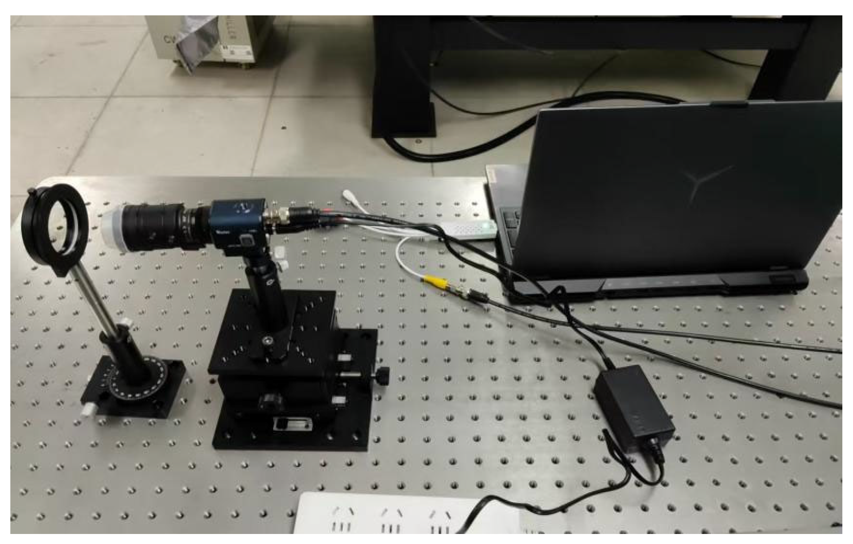
(3) USB video capture card: Figure 3 shows the actual product.
This experiment employed VideoCap4.5 software together with a Watec WAT-902H2 monochrome camera (Watec Co., Ltd., Tsuruoka, Japan) and its imaging lens, which allowed the micro-light polarization image to be clearly displayed on the computer after focusing.
A time-division low-light polarization imaging system was constructed using the aforementioned laboratory equipment. Experimental equipment: microlight cameras, lenses, experimental platforms, computers, polarizers, LiDAR, natural objects, man-made targets. When the illuminance of the target surface met 1 × 10⁻³ lx or was lower than 1 × 10⁻³ lx, the microlight polarizer was driven to rotate according to the four angles of 0 degree, 45 degree, 90 degree and 135 degree for the target scene. The polarized image was acquired through four exposures. After obtaining the low-light polarization image, the Stokes vector imaging formula was used to solve the polarization state of the target scene, and the polarization degree and polarization angle images were obtained. Figure 3 shows the micro-light polarization system.
Rotating actuator: Adopted the TECO DST42-03A two-phase stepper motor from Dongwei Company (Wuxi, China) (step angle 1.8°, rated 1.5A, static torque 0.3 N·m), controlled by a YKA2204MA subdivision driver (Shenzhen YAKO Automation Technology Co., Ltd., Shenzhen, China) (up to 64 subdivisions), with an equivalent step distance of 0.028°/step.
Angle calibration: Used Photon Precision’s PDL-25 laser displacement sensor (Phoskey (Shenzhen) Precision Technology Co., Ltd., Shenzhen, China) (range 25 mm, repeatability 0.02 mm) for closed-loop calibration at four positions: 0°, 45°, 90°, and 135°, with zero drift < 0.05°.
Control core: Used the Qinheng CH32V203C8T6 development board (RISC-V 72 MHz, Nanjing Qinheng Microelectronics Co., Ltd., Nanjing, China), where the angle was reported in real time to the PC through USB-CDC.
Multiple exposure time: Based on the ambient illumination, used 40 ms (maximum SNR without exposure) as the final exposure.
The micro-light polarization imaging system was connected to the computer through the data cable, and the MATLAB2019 software was used to drive the micro-light polarization imaging system and acquire the images in the field of view. For the time-sharing micro-light polarization imaging system, during the debugging process, attention was paid to the time interval between image acquisitions and to avoiding the influence of personnel walking on the ambient light, which in turn affected the experimental conclusions.

3.1.2. LiDAR Imaging System

This research focuses on the multi-sensor matching and fusion of LiDAR and micro-optical camera. In order to improve the matching rate of the subsequently collected data, the data collection for the same target at the same location point should be selected. During the acquisition process, the data quality of the acquired point cloud is observed in real time by ZvisionView V2.3.3 software to ensure the subsequent image processing. Mainly based on the selection of experimental instruments to meet the system design requirements for imaging, the specific hardware is as follows:
(1) LiDAR: ZVISION ML-30S LiDAR (ZVISION, Beijing, China), which has a wavelength of 905nm. With the imaging lens, a clear point cloud image can be obtained. Figure 4 shows the actual product, and Table 2 shows the parameters.
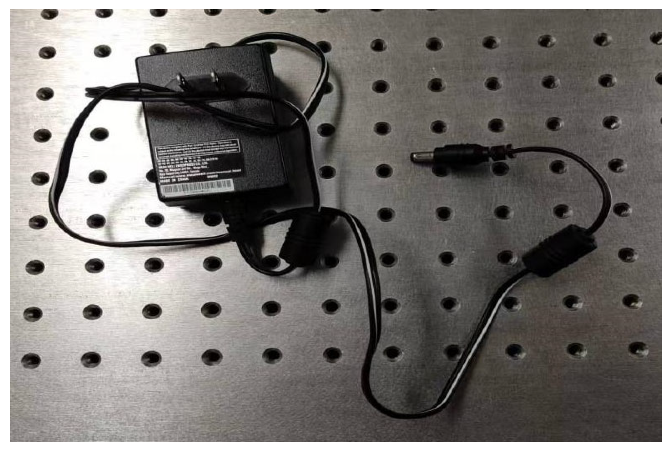
(2) Electrical adapter: Figure 5 shows the actual product.
(3) Ethernet data cable: Standard Ethernet cable.
This experiment uses the ML-30S LiDAR supported by the use of ZvisionView V2.3.3 software with the imaging lens, which can display a clear point cloud image on the computer.
The point cloud information collected in this experiment needs to be preprocessed to remove the clutter. This experiment uses the cloud compare software to preprocess the point cloud in the form of PCD.
For the IP address configuration of the specific steps to open the control panel interface, click to enter the Network and Sharing Center, the “Ethernet” option to jump to the “Ethernet status” interface, click the “Properties” button to enter. Click the “Properties” button. Double-click to select “Internet Protocol Version 4 (TCP/IPv4)” to set the IP address as 192.168.10.1, adjust the subnet mask to 255.255.255.0, and click “Confirm” after all the settings are complete. Click “Confirm” after all the settings are chosen, and then finish setting the IP address of the computer’s network port. To close the firewall, open the computer control panel, enter the System and Security interface, select and open Windows Defender Firewall, select Enable or Disable Windows Defender Firewall, and click Close Windows Defender Firewall. Construct a laser radar imaging system using the existing equipment in the laboratory mentioned above.
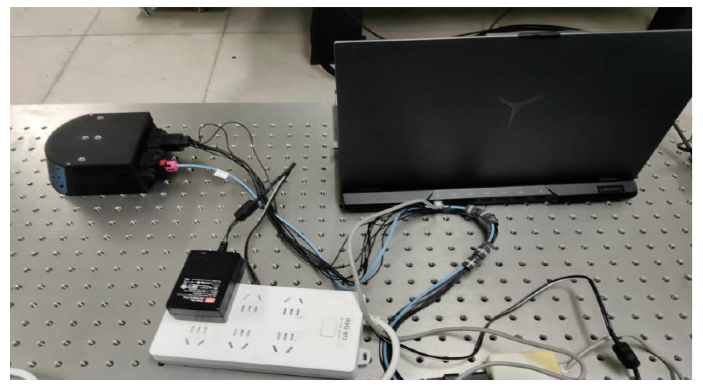
Experimental equipment: LiDAR, electrical adapter, Ethernet data cable, computer, natural objects, man-made targets, etc. Set up the computer network environment configuration, connect LiDAR, computer, start ZvisionView V2.3.3 software, add LiDAR device, play back collected point cloud, and save point cloud data to computer. Figure 6 shows the LiDAR system construction.
System trial acquisition and debugging: Use ZvisionView V2.3.3 software to drive the LiDAR system and acquire data within the field of view. Care is taken to check the LiDAR measurement range to ensure that both the point cloud and the micro-light polarization image fall within this range, preventing mismatches or blind-zone effects that could compromise the subsequent fusion.

3.2. Matching and Fusion Processing

3.2.1. Data Acquisition and Preprocessing

The imaging system must reach a stable state before data acquisition. As the polarizer rotates to different angles, the light intensity varies, causing brightness changes. To eliminate acquisition errors, the system gain is set to 0, ensuring no additional error is introduced. The lens aperture and focal length are then adjusted to obtain a clear image of the target scene, and recording begins.
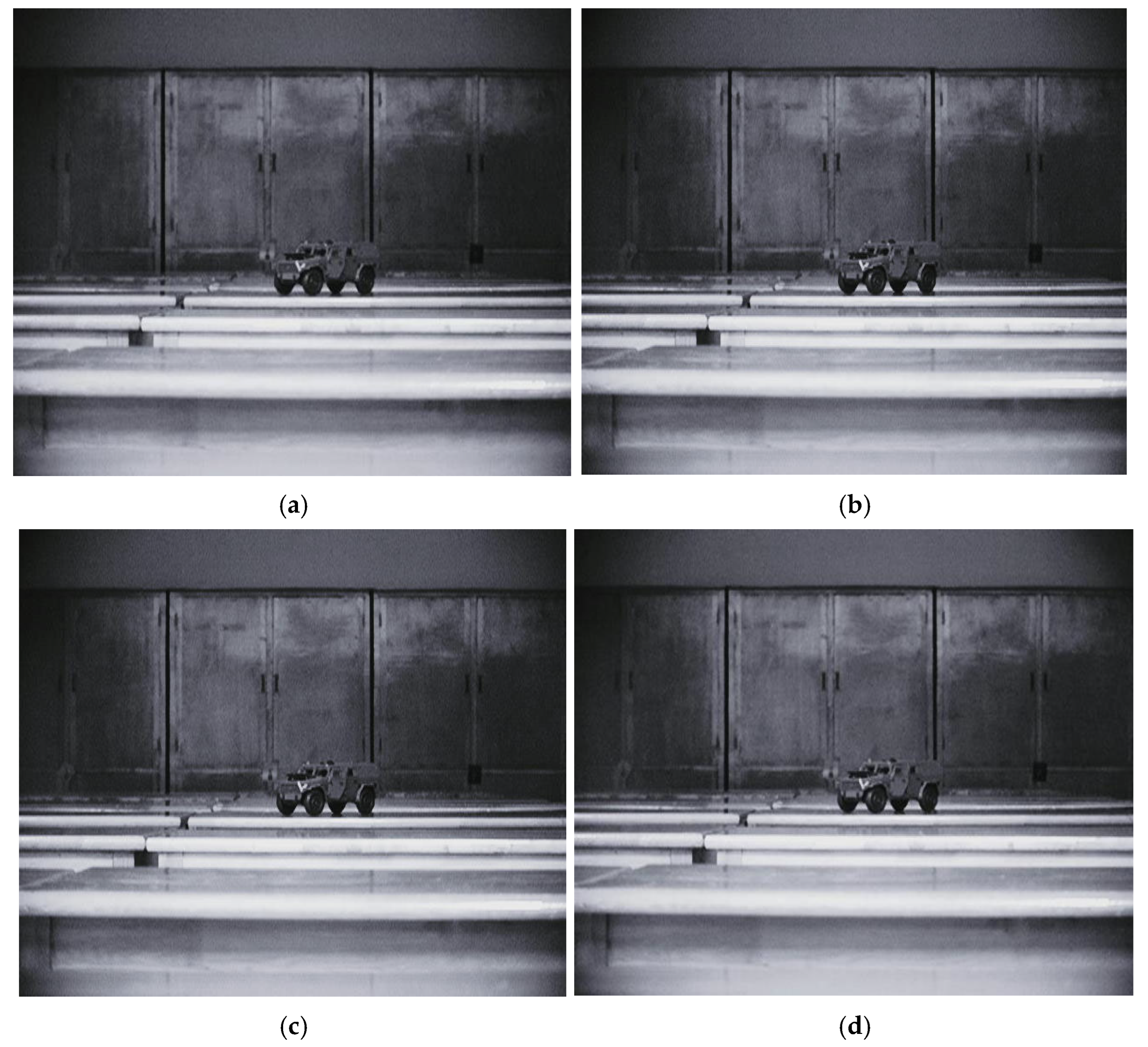
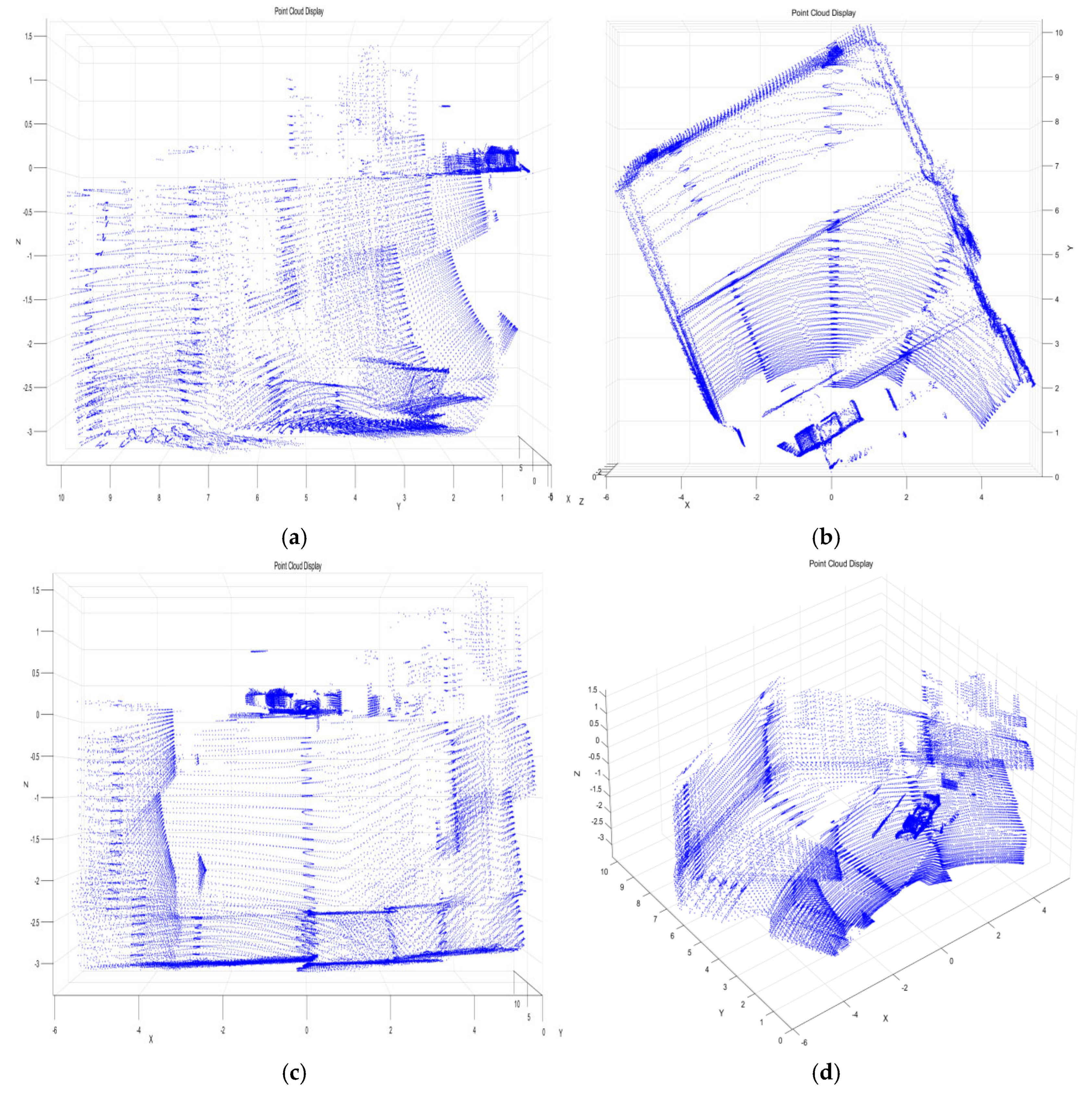
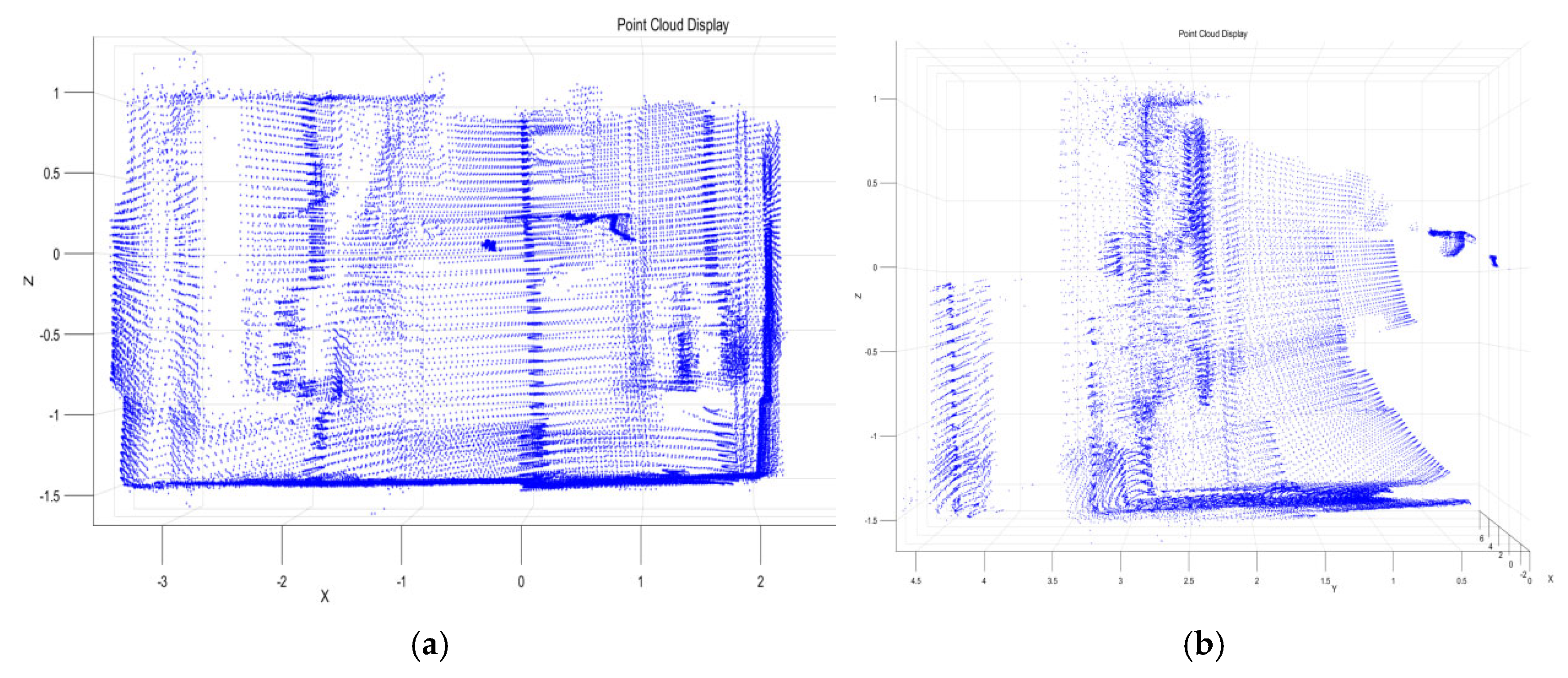
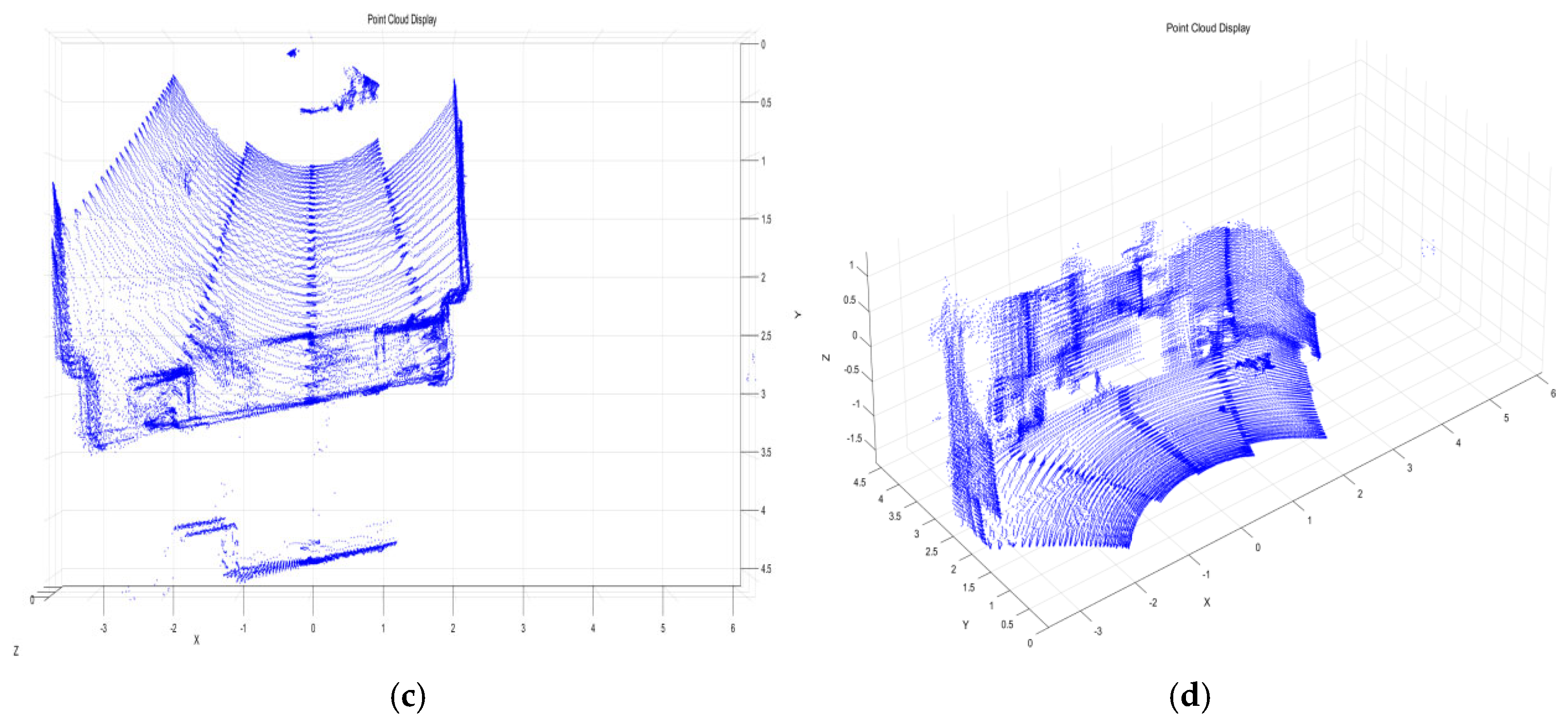
It is essential to note that the time-sequential micro-light polarization system requires careful polarizer adjustment; any vibration introduced during this process can degrade the image quality, obscuring object contours and impairing target recognition. Therefore, a rigid and stable optical platform must be used to avoid experimental errors. Figure 7 shows images acquired at different polarization angles, while Figure 8 presents the pre-acquired point clouds projected onto each plane.
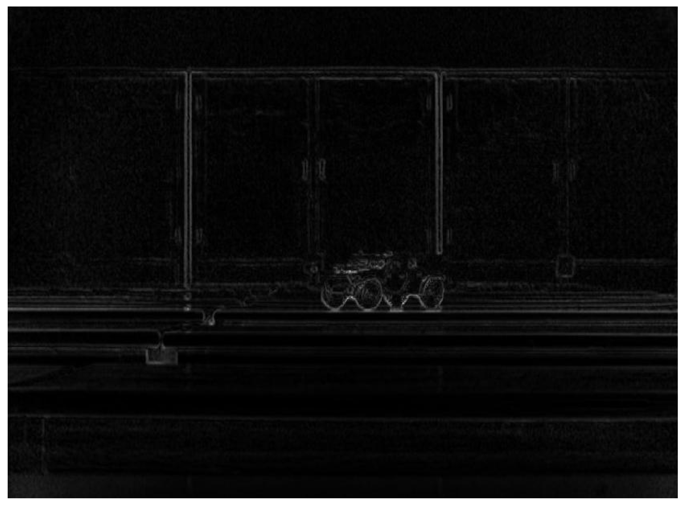
The acquired images at different polarization angles are processed in MATLAB to compute and visualize the Stokes parameters and polarization characteristics, yielding the micro-light polarization image. Figure 9 shows the resulting micro-light polarization image. The micro-light environment and high-gain settings introduce significant grain noise. Stokes vector averaging followed by Gaussian filtering further reduces the noise while preserving the polarization edge information.

3.2.2. LiDAR and Micro-Light Polarization Image Matching

After obtaining the micro-light polarization image, suitable feature points must be matched with those in the point cloud. Because of the large volume of collected point-cloud data, feature point matching faces a heavy computational burden. Therefore, “cloud compare” is employed to remove stray points from the point cloud. The correspondences between the point cloud coordinates and the pixel positions in the micro-light polarization image are then established, and the least squares method is used to solve the 12 elements of the M matrix.
Table 3 shows the calibrated M-parameter matrix elements during pre-acquisition. Among them, SIFT (Scale Independent Feature Transform) is used for feature points, with the main parameters as follows: MaxReginon = 1,320,000, MaxReginon = 80,000, Aspect Ratio = 1~10. Here, a threshold exceeding the threshold is used to automatically remove matching outliers.

3.2.3. LiDAR and Micro-Light Polarization Image Fusion

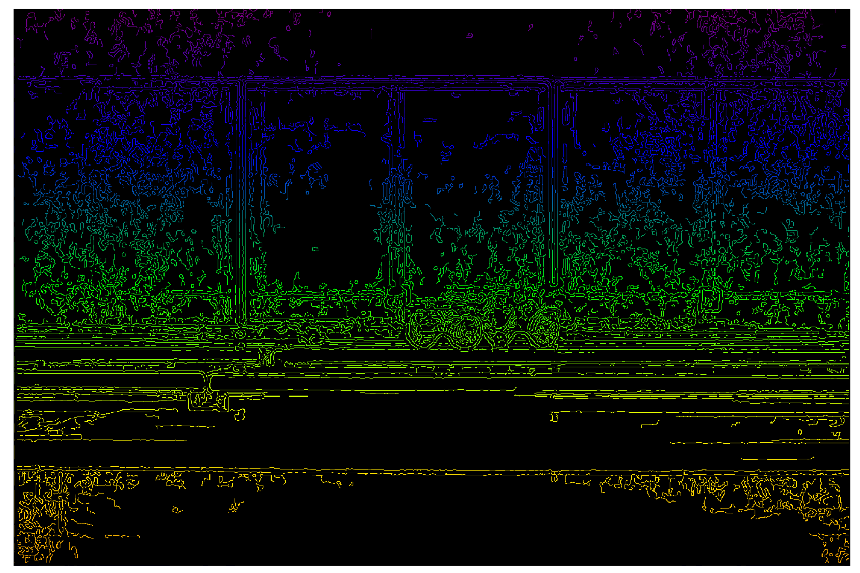
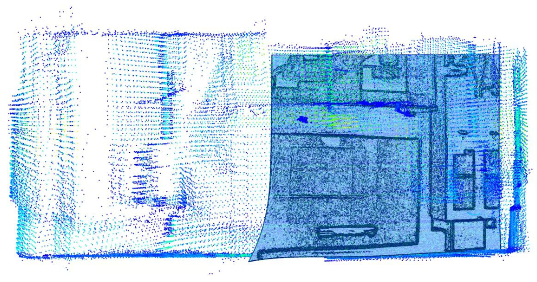
Because the micro-light polarization image is binary, the fused point cloud appears as black and white points that are difficult to interpret and lack surface texture or material cues. Therefore, the Canny operator in MATLAB is applied to extract edge details from the micro-light polarization image, and a gradient color map is assigned to the edges. Figure 10 shows the resulting color-mapped polarization image.
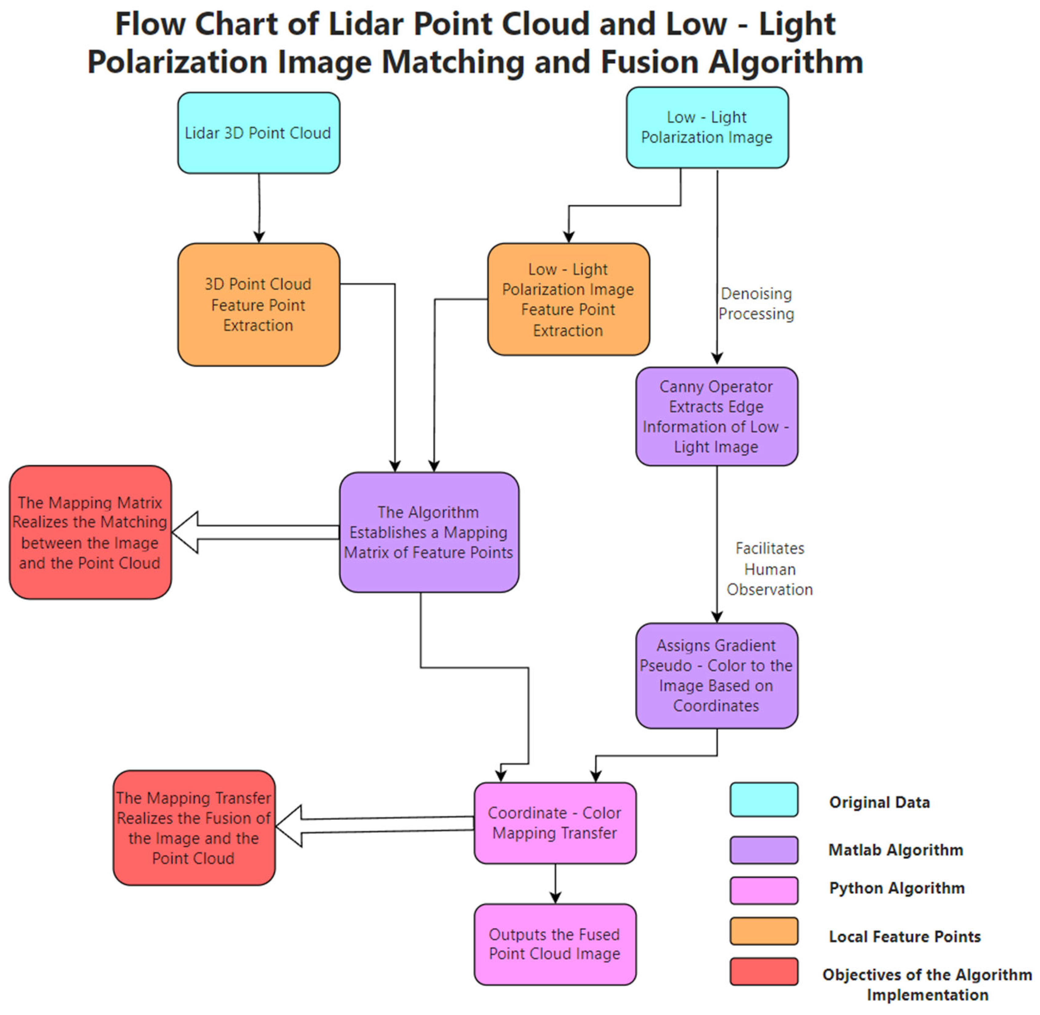
The fusion of point cloud and image is based on the premise of two alignments, where through the alignment of the point cloud and image data, the correspondence between each coordinate point of the point cloud and each pixel of the image has been established. The 3D point cloud is projected onto the optical image to obtain the corresponding pixel coordinates (x, y), and then the corresponding color R, G, and B information at the pixel point (x, y) is assigned to the point cloud, which in turn realizes the coloring of the 3D point cloud data to make it have true color texture information. The MATLAB20192019 software program is used to assign the color information of the micro-light polarization image to the point cloud, so that the pixel position information of the point cloud in the micro-light polarization image can be judged according to the different color information of the point cloud, and then both the texture information of the micro-light polarization and the coordinate information of the point cloud can be displayed on the point cloud image. Figure 11 shows the point cloud image after fusion. Figure 12 shows a flowchart of the matching and fusion algorithm of the LiDAR point cloud and micro-light polarization image.
The fusion effect is shown in Figure 13 by assigning different colors to the micro-light polarization image from top to bottom, so that its color has a mapping relationship with the image pixel coordinates. After the data fusion between the LiDAR point cloud data and the micro-light polarization image, the method of extracting the micro-light polarization image and LiDAR feature points to establish the coordinate matching matrix in Section 2 of this article is used to make the color information in the micro-light polarization image correspond to the corresponding point cloud in the same one-to-one way. Accordingly, it is possible to find the coordinates of the point cloud corresponding to any point of the micro-light polarization image and its spatial position information by searching for the position of any point of the micro-light polarization image and then finding the point cloud coordinates corresponding to any point of the micro-light polarization image according to its corresponding color information. Figure 14 shows a flowchart of the whole system of matching and fusion of the LiDAR and micro-light polarization image. This article requires manual migration from MATLAB2019 to Python.

4. Experiment and Analysis

4.1. Fusion Data

In practical applications, LiDAR is unable to accurately measure a specific target due to its working mechanism. For example, when measuring the target to be measured behind the optical glass, the point cloud cannot show the target to be measured, and the radar point cloud is missing in the area of the target to be measured. In contrast, the micro--light polarization technique can obtain the micro-light polarization image behind the glass. The aim of this research is to display the micro-light polarization image information in the same position radar point cloud coordinate system through the fusion of the LiDAR point cloud and micro-light polarization image. It can make up for the missing point cloud in LiDAR and provide data support for surveyors.
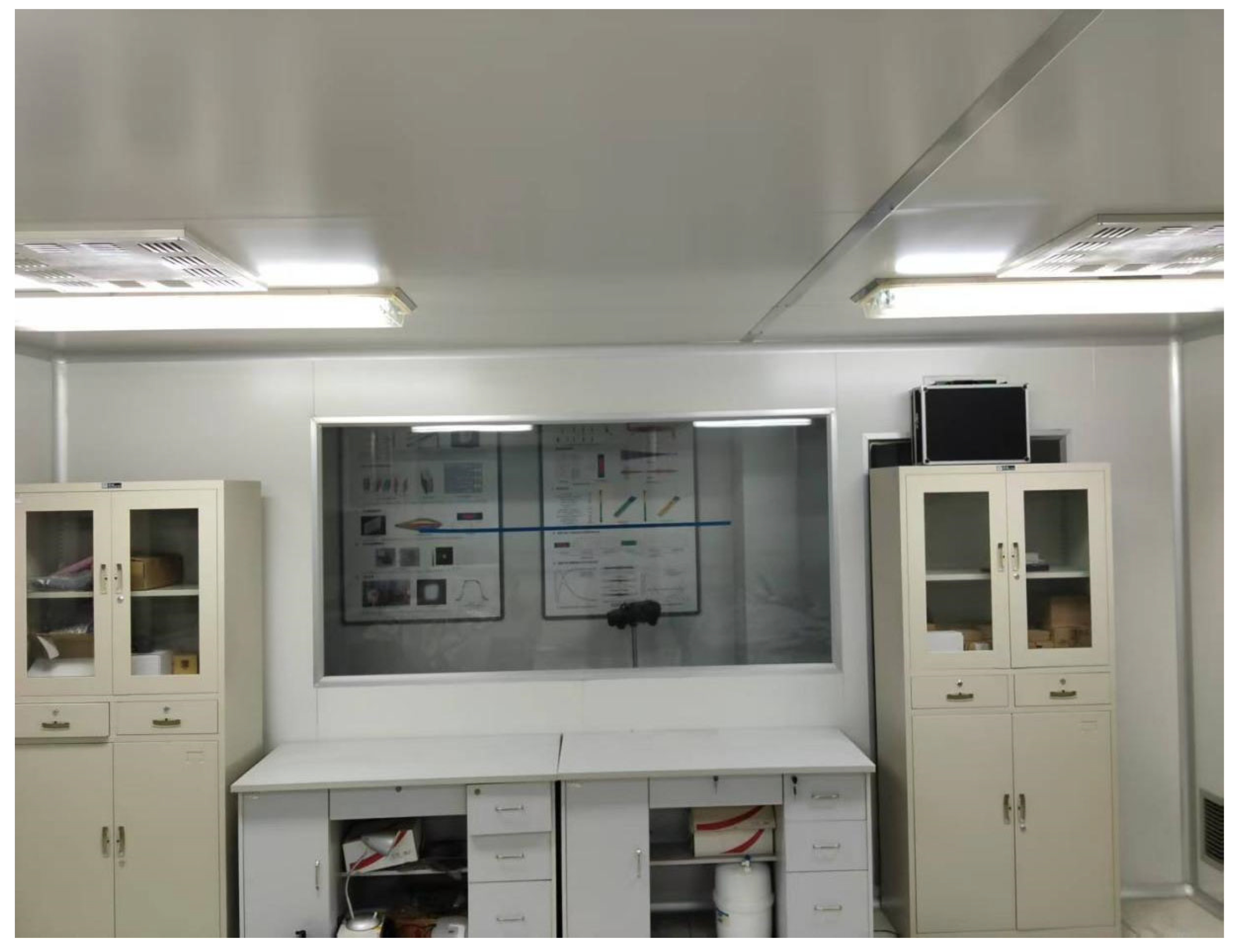
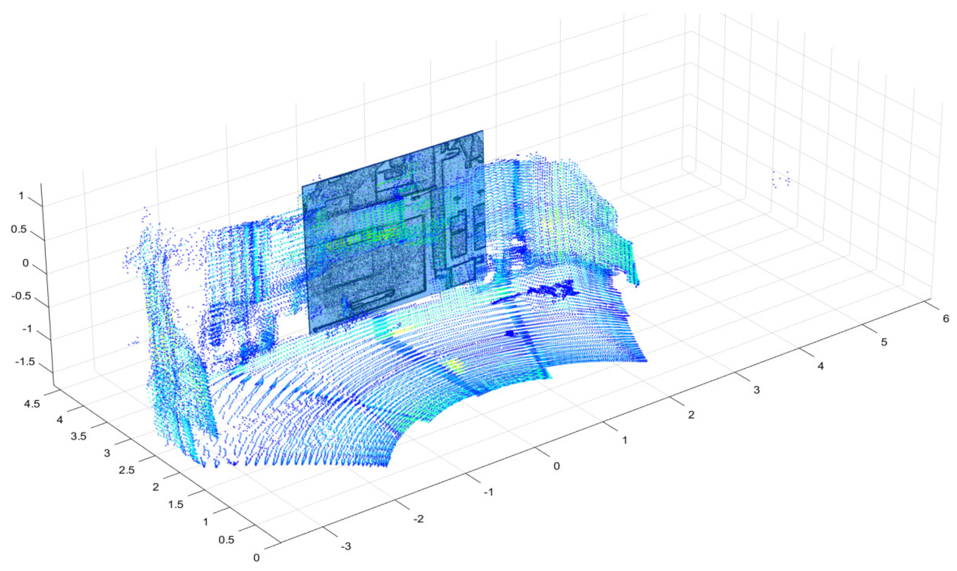
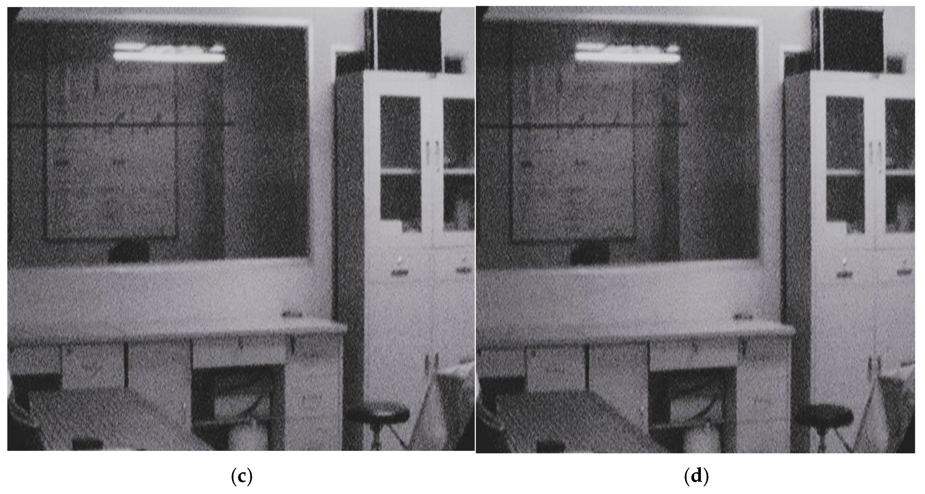
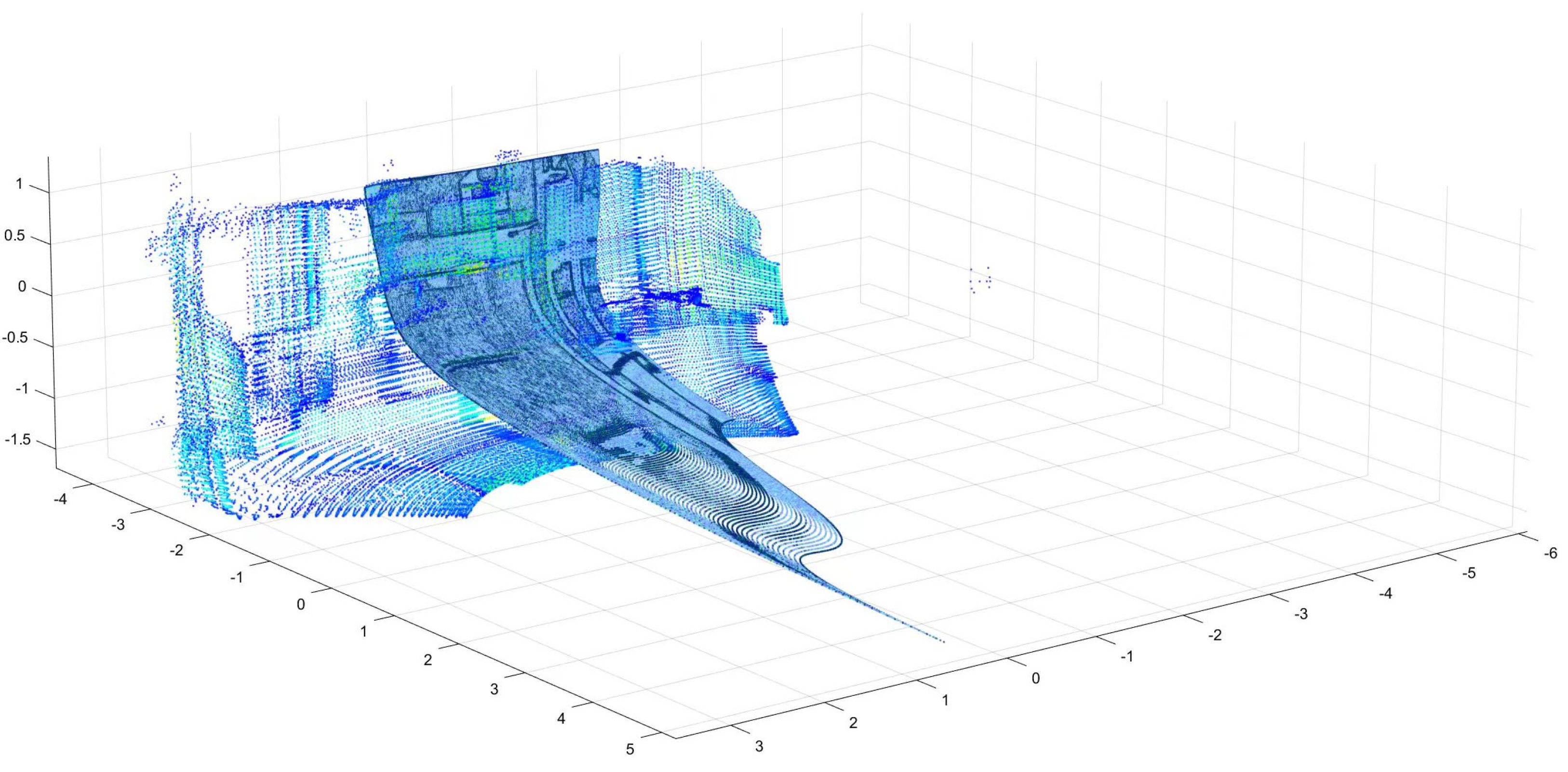
Figure 15 shows the LiDAR point cloud image with optical glass in the scene, and Figure 16 shows the optical glass scene under white light conditions. The point cloud data shows that LiDAR can scan the point cloud data in general scenes, but it cannot detect the target for the back side of the optical glass. In this regard, we can obtain the position information of the glass surface based on the LiDAR point cloud data. Then, we can take the micro-light polarization image of the same scene. After that, we can use the MATLAB2019 software program in Section 1 of this article to process the collected polarization image to obtain the micro-light polarization image. Finally, we use the matching and fusion methods in Section 2 and Section 3 of this article to fuse the LiDAR point cloud image with the micro-light polarization image, so as to obtain the laser point cloud image and micro-light polarization image under the optical glass scene. Finally, using the proposed matching and fusion method, the LiDAR point cloud image is fused with the low-light polarization image to obtain a fused stereo image of the LiDAR and low-light polarization images in optical glass scenes. From Figure 17 and Figure 18, it can be seen that in the fused radar point cloud, both the information of the cart can be displayed and the approximate positional coordinates of the cart as well as the 3D spatial layout can be determined. Of course, since the relative positions of the LiDAR and the low-light camera may change during the acquisition process, the micro-light polarization image and the 3D point cloud need to be re-matched before fusion. The grainy noise apparent in Figure 19 is dominated by sensor read-out noise. Slight mechanical vibrations during the time-division rotation of the polarizer, combined with the high AGC gain, amplify the random noise, resulting in consistent bright and dark speckles across all four polarization angle images.
Polarization image processing is performed on images collected at different polarization angles, the Stokes parameters and polarization characteristics are calculated and visualized, and the processed low-light polarization images are obtained. Figure 19 shows polarization angle images for each polarization angle in the optical glass scene. Figure 20 shows the processed low-light polarization image.
From the LiDAR and micro-light polarization images, it is easy to find out that the LiDAR cannot measure the object behind the optical glass, while the micro-light polarization image can display the information of the object behind. Using the matching and fusion methods, which need to be re-matched due to changes in the relative positions of the LiDAR and the low-light camera during the acquisition process, the fused point cloud displays information about the cart and can determine the approximate positional coordinates of the cart as well as the 3D spatial layout.

4.2. Matching Effect Evaluation

For the evaluation of the micro-light polarization image and LiDAR point cloud matching, it is necessary to consider both the matching rate and the error of the micro-light polarization image and LiDAR point cloud matching results. Due to the reflection of laser by glass, LiDAR cannot collect point cloud data behind the glass, which means that the radar point cloud is missing the data behind the glass. Micro-light polarization images are designed to compensate for the missing data in low-light environments. When filling in missing data, we are more concerned about the spatial or structural consistency between the image data being filled and the missing data in the radar point cloud. Therefore, it is better to select the “geometric consistency” evaluation metric—the matching rate—as well as the maximum and average position errors as the evaluation parameters to analyze the data quality after matching.
(1) The matching rate reflects the accuracy of the cross-modal feature alignment, that is, the ratio of the number of pairs of feature points successfully matched to the total number of pairs of detected feature points. The more feature points that are successfully matched, the larger the matching rate is, and the better the matching quality is.
R = N correct N total × 100 %
where Ncorrect denotes the number of feature point pairs correctly matched and Ntotal denotes the number of feature point pairs of the total matching attempts.
(2) The maximum error reflects the limit value of the degree of inaccurate matching, that is, the maximum value of single point deviation among all the corresponding point pairs (or feature pairs) in the matching or fusion result.
E max = max u i u i 2 + v i v i 2
where (ui, vi) are the pixel coordinates of the point cloud mapped on the micro-light polarization image, and (ui′, vi′) are the corresponding 2D coordinates manually labeled in the image.
(3) The average error reflects the average degree of matching inaccuracy.
E average = 1 N i = 1 N u i u i 2 + v i v i 2
where (ui, vi) are the pixel coordinates of the point cloud mapped on the micro-light polarization image, (ui′, vi′) are the corresponding 2D coordinates manually labeled in the image, and N is the number of matching points.
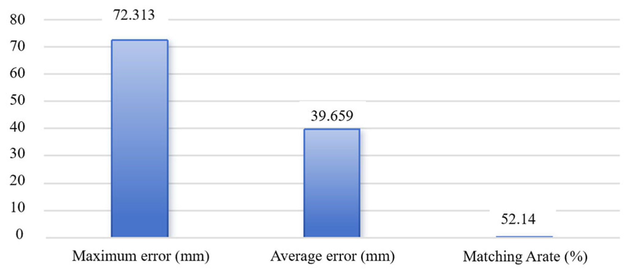
According to Equations (8)–(10), the evaluation of the effect of matching the LiDAR point cloud with the micro-light polarization in Figure 16, respectively. The Statistical data is showed in Figure 21.
As can be seen from Figure 21, the matching rate between the micro-light polarization image and the LiDAR point cloud in the experiment shown in Figure 19 is 52.14%, the maximum error is 72.313 mm, and the average error is 39.659 mm, which basically achieves the matching effect.

4.3. System Optimization

As can be seen from Figure 21, the mapping matrix of the micro-light polarization image and LiDAR point cloud is established based on the feature points. Although the matching purpose is initially realized, the matching rate is not high and the error is relatively large. Accordingly, several system optimization schemes are proposed.

4.3.1. System Design Optimization

The system can be divided into multiple modules, such as data acquisition, preprocessing, matching and fusion, to facilitate independent optimization and maintenance. In the micro-light polarization imaging system, the different illumination of the scene affects the imaging quality of each polarization degree, which in turn affects the micro-light polarization image. Therefore, the imaging quality of the micro-light polarization image under different illumination conditions can be analyzed experimentally to find out the corresponding illumination when the micro-light polarization imaging effect is optimal, which can be used to guide the subsequent experimental operation.

4.3.2. Optimization of the System Feature Extraction Algorithm

The point cloud matching in this study is based on geometric features, which have been disturbed in the low-light environment. For example, the introduction of polarization features fused with geometric features or the construction of new feature vectors using the polarization degree and polarization angle can significantly improve the accuracy of feature extraction. Meanwhile, only local feature points are selected in the feature matching in this study, which are limited in number, and there is a matching error when matching the micro-light polarization with LiDAR.
Accordingly, the optimized system feature extraction algorithm is designed. Firstly, for the flickering polarized image, the Stokes parameters are calculated to obtain the polarization degree and polarization angle. Secondly, the reflective intensity of each point cloud in the LiDAR point cloud data is extracted. Finally, a mapping relationship is established by finding the polarization degree and polarization angle information of each point cloud point reflection intensity with the corresponding pixel polarization degree and polarization angle information on the polarization image to correlate the polarization degree and polarization angle information with the point cloud reflection intensity.
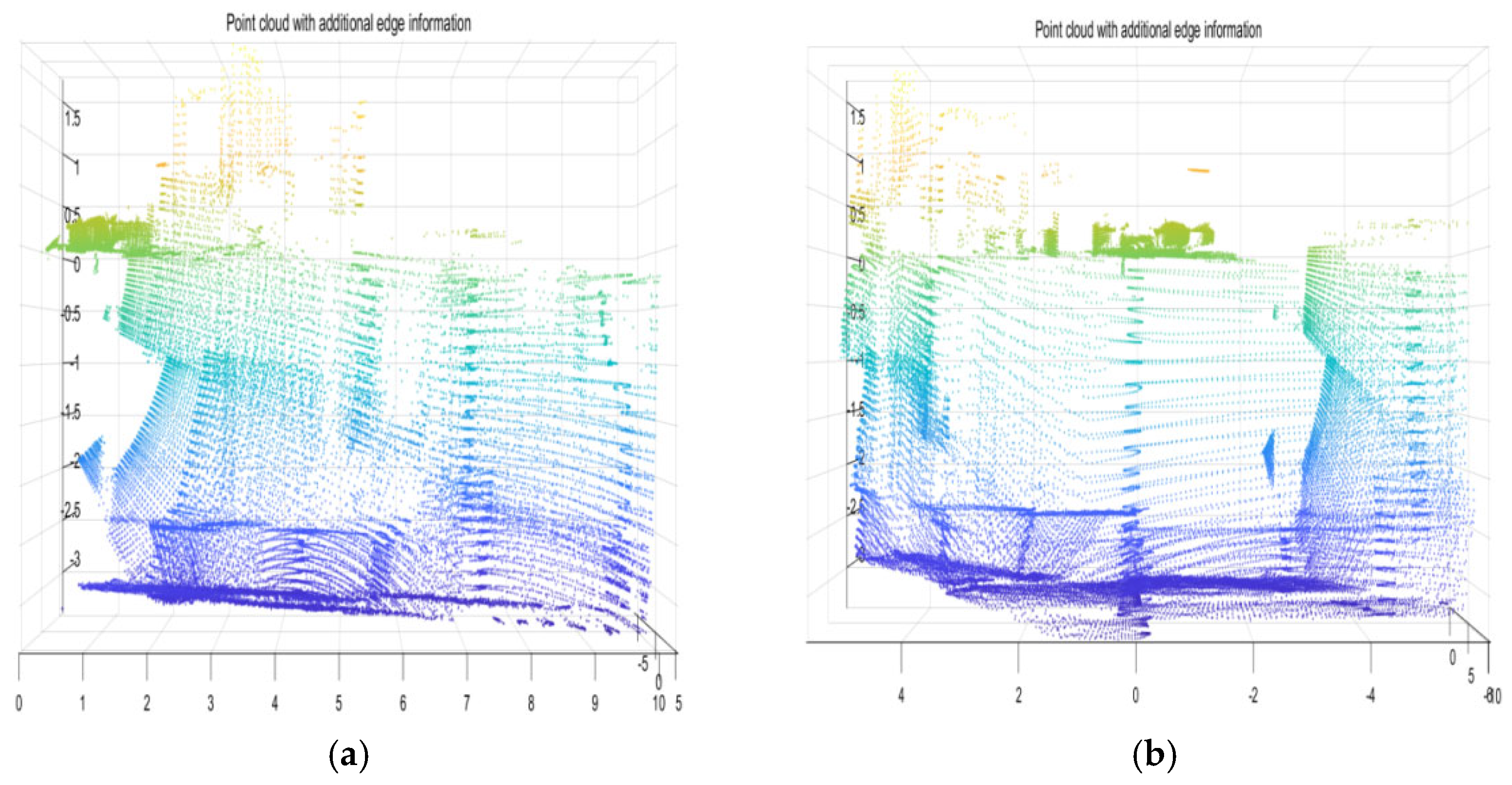
After the optimization of the algorithm, on the basis of the original extraction of pixel coordinates, the extraction of vectors such as the polarization degree and polarization angle of the pixels of the polarized image, as well as the extraction of the reflection intensity of the points of each point cloud of the LiDAR, is also added. Figure 22 and Figure 23 show the fusion of the LiDAR and micro-light polarization images after the optimization of the mapping relationship between the polarization information vectors and the reflection intensity of the point cloud.
Firstly, as can be seen from Figure 22, the front view of the micro-light polarization image in the new fusion map remains unchanged after system optimization, and the detail information of its micro-light polarization image is retained. Secondly, in Figure 23 and Figure 24, the curved part of the micro-light polarization image is highly matched with the point cloud data in the radar point cloud, and the fusion effect of the radar point cloud and the micro-light polarization image is better. The matching effect is also tested. From Figure 25, it can be seen that the matching rate of the feature points is improved and the system error is reduced. At the same time, we also use standard point-to-point ICP as a control, and the experimental conditions are completely consistent with the method proposed in this paper (same point cloud, same feature point set). The comparison results of the matching effects are shown in Table 4. Compared with standard ICP, the method proposed in this paper exhibits a higher matching rate and lower reprojection error in low-light and low-texture scenes, verifying the effectiveness of using polarization information to improve cross-modal registration.
However, systematic errors are introduced during data processing and matching optimization. During mapping and fusion based on the polarization degree, polarization angle, and LiDAR reflectance intensity, the algorithm may employ approximations or simplifications, leading to image deformation (e.g., curved poles in Figure 23). The LiDAR scene is assembled from overlapping partial point clouds. Overlapping partial clouds inevitably alter the original reflectance values. Using these altered reflectance values for polarization mapping causes excessive bending and deformation.

4.3.3. System Response Optimization

Due to the limitations of the time-sequential micro-light polarization system, we can leverage GPU acceleration and multithreading to improve the system response speed. For example, the GPU hardware can use the Moore Thread MTT S4000 (Moore Threads Technology Co., Ltd., Beijing, China). The parallel framework can use Moore’s Thread MUSA Toolkit 2.3 to compile the core operators (Stokes vector computation, point cloud projection) into PTX through mucc and call them using MATLAB R2023b’s gpuArray+parallel.gpu.CUDANel. In terms of the thread allocation strategy, on the CPU side, MATLAB parpool (“local”, 12) can be used for outlier removal; on the GPU side, each 640 × 480 image block is processed in parallel with 1024 × 1 × 1 thread block.

5. Conclusions

In this paper, for the problem of LiDAR being unable to generate point clouds for the area behind the glass, a method of fusing the micro-light polarization image with the laser LiDAR point cloud is proposed to realize the reconnaissance, identification and ranging method for the blind area of the point cloud caused by transparent media such as glass in low illumination environments. The method optimizes the 3D point cloud generated from the micro-light polarization image by introducing the polarization degree, polarization angle, and reflection intensity of each point of the LiDAR and constructing a point cloud–pixel mapping matrix that contains a depth offset and a better fit on the basis of extracting the pixel coordinates of the 3D LiDAR point cloud. Subsequently, with the help of 3D point cloud fusion and the pseudo-color mapping algorithm, the matching and fusion algorithm of the micro-light polarization map and the radar point cloud are further optimized, and the alignment and fusion of the 2D micro-light polarization map and the 3D LiDAR point cloud are successfully completed. Experiments show that the alignment rate of the two reaches 74.82%, which can effectively detect hidden targets behind the glass under low illumination conditions while compensating for the blind spot of the LiDAR point cloud data, verifying the feasibility of “Polarization + LiDAR” reconnaissance in low illumination glass scenes and providing new ways of detecting hidden targets in complex environments. It provides a new means of hidden target detection in complex environment.
This study validates the effectiveness of micro-light-polarization–LiDAR fusion for glass-occlusion detection in static, low-light scenes, but it still has the following limitations:
First, feature point selection relies on a limited sample size, introducing randomness and leading to substantial errors and low accuracy when matching low-light polarization images with LiDAR point clouds.
Second, dynamic scene adaptability is limited: the current time-division polarizer requires four sequential exposures, causing motion blur in moving targets and increasing feature point mismatches.
Third, remote detection accuracy degrades with distance: the ML-30S LiDAR point density declines sharply, while the SNR of micro-light polarization images falls with the square of the distance, thereby increasing the matching errors.
Future work will be carried out from the following three aspects. Matching optimization: increase the number of feature points and optimize the point cloud matching process. Dynamic perception: develop a snapshot polarization camera based on a liquid crystal adjustable polarizer (μs-level switching), combined with an event camera to achieve blur free imaging of moving targets. Of course, a split aperture acquisition system can also be used to attempt real-time acquisition of polarization images using four channels simultaneously. Remote enhancement: introduce high-power fiber lasers and dual axis MEMS scanning to effectively expand the detection range; simultaneously using multiple frames of polarized image super-resolution reconstruction to improve SNR.

Author Contributions

Conceptualization, J.Y. and G.L.; data curation, J.Y.; formal analysis, J.Y.; funding acquisition, J.Y.; investigation, J.Y. and B.Z.; methodology, J.Y. and L.C.; project administration, J.Y. and G.L.; resources, B.Z.; software, J.Y.; supervision, G.L. and B.Z.; validation, B.Z.; visualization, J.Y. and G.L.; writing—original draft, J.Y. and L.C.; writing—review and editing, J.Y. and G.L. All authors have read and agreed to the published version of the manuscript.

Funding

This research received no external funding.

Data Availability Statement

The dataset was obtained by the authors and related personnel through the joint experiment with the field imaging spectrometer. The data belongs to the Department of Electronic and Optical Engineering of the Army University of Engineering. It is not a public dataset. The data are not made public due to copyright issues.

Conflicts of Interest

The authors declare no conflicts of interest. The funders had no role in the design of the study; in the collection, analyses, or interpretation of data; in the writing of the manuscript, or in the decision to publish the results.

References

  1. Wei, J.; Che, K.; Gong, J.; Zhou, Y.; Lv, J.; Que, L.; Liu, H.; Len, Y. Fast and Accurate Detection of Dim and Small Targets for Smart Micro-Light Sight. Electronics 2024, 13, 3301. [Google Scholar] [CrossRef]
  2. Li, S.; Kong, F.; Xu, H.; Guo, X.; Li, H.; Ruan, Y.; Cao, S.; Guo, Y. Biomimetic Polarized Light Navigation Sensor: A Review. Sensors 2023, 23, 5848. [Google Scholar] [CrossRef]
  3. Wang, P.; Liu, Y.; Liang, X.; Zhu, D.; Gong, X.; Ye, Y.; Lee, H.F. CIRSM-Net: A Cyclic Registration Network for SAR and Optical Images. IEEE Trans. Geosci. Remote Sens. 2025, 63, 5610619. [Google Scholar] [CrossRef]
  4. Liu, D.; Xu, C.; Li, Y.; Song, A.; Li, J.; Jin, K.; Luo, X.; Wei, K. Laser Phase Noise Compensation Method Based on Dual Reference Channels in Inverse Synthetic Aperture Lidar. Remote Sens. 2025, 17, 30. [Google Scholar] [CrossRef]
  5. Su, Y.; Shao, S.; Zhang, Z.; Xu, P.; Cao, Y.; Cheng, H. GLO: General LiDAR-Only Odometry With High Efficiency and Low Drift. IEEE Robot. Autom. Lett. 2025, 10, 3518–3525. [Google Scholar] [CrossRef]
  6. Yao, Y.; Ishikawa, R.; Oishi, T. Stereo-LiDAR Fusion by Semi-Global Matching With Discrete Disparity-Matching Cost and Semidensification. IEEE Robot. Autom. Lett. 2025, 10, 4548–4555. [Google Scholar] [CrossRef]
  7. Song, A.; Liu, D.; Zhang, Y.; Li, J.; Wang, C.; Chen, H. Impact of Phase Error on Coherent LiDAR: Analysis and Validation. J. Light. Technol. 2025, 43, 4149–4155. [Google Scholar] [CrossRef]
  8. Herraez, D.C.; Zeller, M.; Wang, D.; Behley, J.; Heidingsfeld, M.; Stachniss, C. RaI-SLAM: Radar-Inertial SLAM for Autonomous Vehicles. IEEE Robot. Autom. Lett. 2025, 10, 5257–5264. [Google Scholar] [CrossRef]
  9. Joseph, T.; Fischer, T.; Milford, M. Matched Filtering Based LiDAR Place Recognition for Urban and Natural Environments. IEEE Robot. Autom. Lett. 2025, 10, 2566–2573. [Google Scholar] [CrossRef]
  10. Chai, L.; Wang, W.; Li, C.; Zhu, L.; Li, Y. Simultaneous Localization and Mapping Method for LiDAR and IMU Using Surface Features. Laser Optoelectron. Prog. 2025, 62, 0415004. [Google Scholar] [CrossRef]
  11. Li, J.; Xu, W.; Shi, P.; Zhang, Y.; Hu, Q. LNIFT: Locally Normalized Image for Rotation Invariant Multimodal Feature Matching. IEEE Trans. Geosci. Remote Sens. 2022, 60, 5621314. [Google Scholar] [CrossRef]
  12. Zhang, J.; Singh, S. Low-drift and Real-time LiDAR Odometry and Mapping. Auton. Robot. 2017, 41, 401–416. [Google Scholar] [CrossRef]
  13. Vizzo, I.; Guadagnino, T.; Mersch, B.; Wiesmann, L.; Behley, J.; Stachniss, C. KISS-ICP: In Defense of Point-to-Point ICP—Simple, Accurate, and Robust Registration If Done the Right Way. IEEE Robot. Autom. Lett. 2023, 8, 1029–1036. [Google Scholar] [CrossRef]
  14. Jia, S.; Zhou, X.; Jiang, S.; He, R. Collaborative Contrastive Learning for Hyperspectral and LiDAR Classification. IEEE Trans. Geosci. Remote Sens. 2023, 61, 5507714. [Google Scholar] [CrossRef]
  15. Cui, Y.; Chen, R.; Chu, W.; Chen, L.; Tian, D.; Li, Y.; Cao, D. Deep Learning for Image and Point Cloud Fusion in Autonomous Driving: A Review. IEEE Trans. Intell. Transp. Syst. 2022, 23, 722–739. [Google Scholar] [CrossRef]
  16. Chitta, K.; Prakash, A.; Jaeger, B.; Yu, Z.; Renz, K.; Geiger, A. TransFuser: Imitation With Transformer-Based Sensor Fusion for Autonomous Driving. IEEE Trans. Pattern Anal. Mach. Intell. 2023, 45, 12878–12895. [Google Scholar] [CrossRef]
  17. Hang, R.; Li, Z.; Ghamisi, P.; Hong, D.; Xia, G.; Liu, Q. Classification of Hyperspectral and LiDAR Data Using Coupled CNNs. IEEE Trans. Geosci. Remote Sens. 2020, 58, 4939–4950. [Google Scholar] [CrossRef]
  18. Zhang, D.; Liang, J.; Guo, C.; Chen, Z.; Liu, J.; Zhang, X. Integrated Precision Evaluation Method for 3D Optical Measurement System. Proc. Inst. Mech. Eng. Manuf. 2011, 225, 909–920. [Google Scholar] [CrossRef]
  19. Li, M.; Yang, W.; Chen, W.; Li, Z.; Li, Y.; Ma, T.; Hu, X.; Ma, L. Deep-Learning-Based Point Cloud Completion Methods: A Review. Graph. Models 2024, 136, 101233. [Google Scholar]
  20. Liu, H.; Wu, Y.; Li, A.; Deng, Y. Precision Detection and Identification Method for Apparent Damage in Timber Components of Historic Buildings Based on Portable LiDAR Equipment. J. Build. Eng. 2024, 98, 111050. [Google Scholar] [CrossRef]
  21. Dong, Q.; Wei, T.; Wang, Y.; Zhang, Q. Intangible Cultural Heritage Based on Finite Element Analysis: Force Analysis of Chinese Traditional Garden Rockery Construction. Herit. Sci. 2024, 12, 241. [Google Scholar] [CrossRef]
  22. Zhu, Q.; Wang, X.; Li, Y.; Chen, Y.; Liu, H.; Zhang, J. Advancements in point cloud data augmentation for deep learning: A survey. Pattern Recognit. 2024, 153, 110532. [Google Scholar] [CrossRef]
  23. Hao, M.; Zhang, Z.; Li, L.; Dong, K.; Cheng, L.; Tiwari, P.; Ning, X. Coarse to Fine-Based Image–Point Cloud Fusion Network for 3D Object Detection. Inf. Fusion 2024, 112, 102551. [Google Scholar] [CrossRef]
  24. Feng, Y.; Li, H.; Li, C.; Chen, J. 3D Modelling Method and Application to a Digital Campus by Fusing Point Cloud Data and Image Data. Heliyon 2024, 10, e36529. [Google Scholar] [CrossRef]
  25. Zhang, B.; Su, C.; Cao, G. Enhanced DetNet: A New Framework for Detecting Small and Occluded 3D Objects. Electronics 2025, 14, 979. [Google Scholar] [CrossRef]
  26. Li, W.; Li, F.; Wang, H.; Huang, Y.; Zhang, Z.; Xie, Q.; Gao, X. Fringe Projection Profilometry(FPP) Based Point Clouds Fusion for the Binocular and Monocular Structured Light Systems. J. Opt. 2024, 1–11. [Google Scholar] [CrossRef]
  27. Zhang, J.; Tang, Y.; Bian, Z.; Sun, T.; Zhong, K. Fusion and Visualization of Three-Dimensional Point Cloud and Optical Images. Laser Optoelectron. Prog. 2023, 60, 0611001. [Google Scholar]
  28. Luo, H.; Zhang, J.; Gai, X.; Wang, K.; Li, Y.; Chen, J.; Li, Y. Development Status and Prospects of Polarization Imaging Technology (Invited). Infrared Laser Eng. 2022, 51, 20210987. [Google Scholar]
  29. Zhang, J.; Chen, J.; Luo, H.; Li, Y.; Wang, K.; Gai, X. Polarization Image Interpolation Algorithm via Tensor Non-Negative Sparse Factorization. Acta Opt. Sin. 2021, 41, 1411001. [Google Scholar]
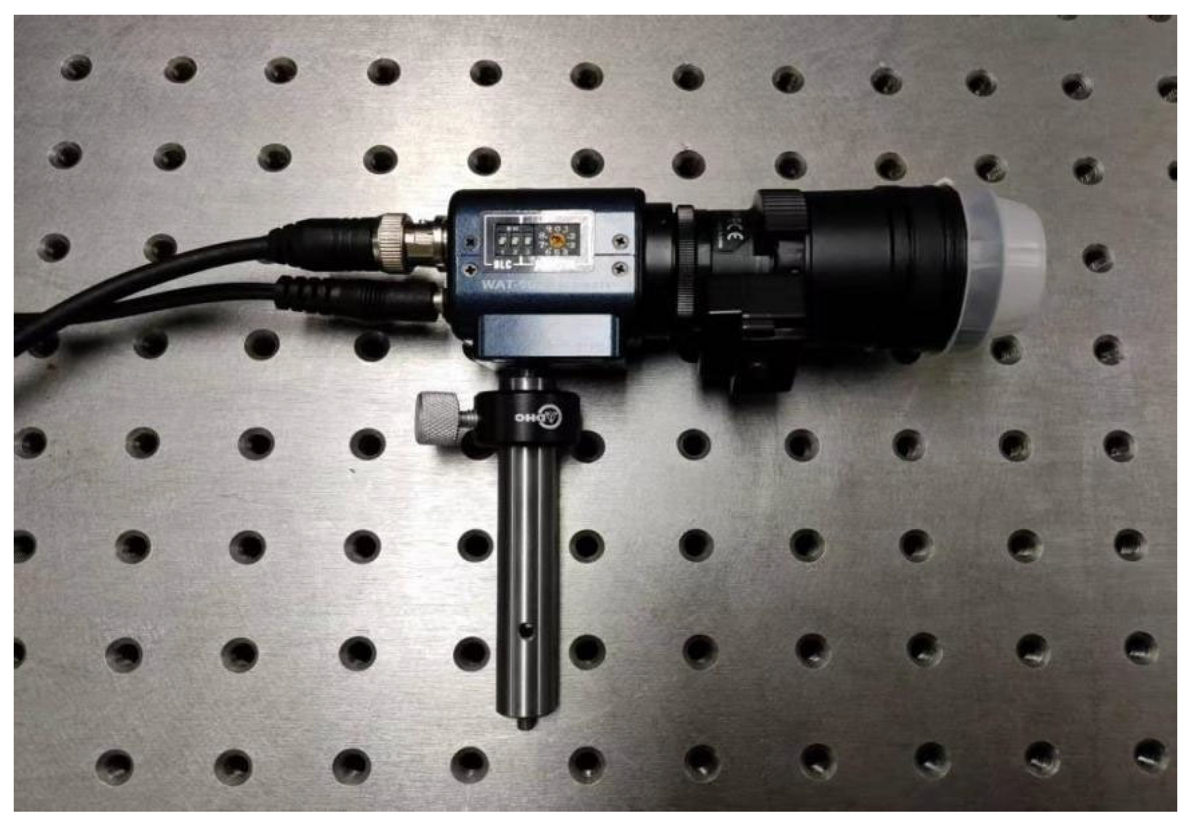
Figure 1. Watec WAT-902H2 black and white camera.
Electronics 14 03136 g001
Figure 2. Polarizer.
Electronics 14 03136 g002
Figure 3. Micro-light polarization system.
Electronics 14 03136 g003
Figure 4. ML-30S LiDAR.
Electronics 14 03136 g004
Figure 5. Electrical adapter.
Electronics 14 03136 g005
Figure 6. LiDAR system construction.
Electronics 14 03136 g006
Figure 7. Original low-light polarization images with different polarization angles: (a) 0 degree, (b) 45 degrees, (c) 90 degrees, and (d) 135 degrees.
Electronics 14 03136 g007
Figure 8. Experimental pre-collection of the point cloud obtained by the projection of each plane. (a) Main view. (b) Top view. (c) Left view. (d) Cubic view.
Electronics 14 03136 g008
Figure 9. Pre-micro-light polarization image after processing.
Electronics 14 03136 g009
Figure 10. The resulting color-mapped polarization image.
Electronics 14 03136 g010
Figure 11. Point cloud image after fusion. (a) Main view. (b) Left view. (c) Top view. (d) Stereo view.
Electronics 14 03136 g011aElectronics 14 03136 g011b
Figure 12. Flowchart of the matching and fusion algorithm of the LiDAR point cloud and micro-light polarization image.
Electronics 14 03136 g012
Figure 13. Coordinates of the fused point cloud image and the micro-light polarization image.
Electronics 14 03136 g013
Figure 14. Flowchart of the whole system of matching and fusion of the LiDAR and micro-light polarization image.
Electronics 14 03136 g014
Figure 15. Preprocessing results of the point cloud multi-plane projection in optical glass scenes. (a) Main view. (b) Left view. (c) Top view. (d) Stereo view.
Electronics 14 03136 g015aElectronics 14 03136 g015b
Figure 16. White light image in optical glass scene.
Electronics 14 03136 g016
Figure 17. Fusion of LiDAR and micro-light polarization three-dimensional map in optical glass scene.
Electronics 14 03136 g017
Figure 18. Fusion of LiDAR and micro-light polarization image in optical glass scene.
Electronics 14 03136 g018
Figure 19. Original low-light polarization images with different polarization angles in the optical glass scene: (a) 0 degree, (b) 45 degrees, (c) 90 degrees, and (d) 135 degrees.
Electronics 14 03136 g019aElectronics 14 03136 g019b
Figure 20. Processed low-light polarization image in optical glass scene. (a) Polarization degree. (b) DoP polarization angle AoP.
Electronics 14 03136 g020
Figure 21. Evaluation of the effect of matching the LiDAR point cloud with the micro-light polarization image.
Electronics 14 03136 g021
Figure 22. Front view of the image after system optimization.
Electronics 14 03136 g022
Figure 23. Stereo view of the image after system optimization.
Electronics 14 03136 g023
Figure 24. Image effect after system optimization.
Electronics 14 03136 g024
Figure 25. Matching error distribution before and after system optimization. (a) Error distribution before registration. (b) Error distribution after registration.
Electronics 14 03136 g025
Table 1. Specific parameters of micro-light camera.
Minimum IlluminationSignal-to-Noise Ratio Gain Mode
0.0003 LuxF1.4 (AGC:High)46 dBAutomatic
Table 2. Specific parameters of ML-30S LiDAR.
Machine versionML-30s B1
FOV (°)Horizontal FOV: 140° (70°~+70°)
Vertical FOV: 70° (FOV1: −10°~+20°)
(fov2: −50°~−10°)
Detection distance (m)100 k LuxResolutionHXV: 320 × 160
Maximum detection distance (m)40 mMinimum detection distance (m)20 cm
Frame rate (FPS)10Data interface100Base-T1
(data: UDP; control: TCP)
Data TypeDistance, reflectivity, azimuth and altitude AnglePoints per second512,000 points per second
Table 3. Calibrated M-parameter matrix elements during pre-acquisition.
−0.04235−3.4568670.09169.1191
02.67046105.673622
06.91601706.666525
Table 4. Comparison of matching effects before and after optimization.
MethodMatching Rate (%)Average Error (mm)Maximum Error (mm)
Original method52.1439.65972.313
Optimizing method74.8221.89363.256
Standard ICP60.3730.88068.934
Disclaimer/Publisher’s Note: The statements, opinions and data contained in all publications are solely those of the individual author(s) and contributor(s) and not of MDPI and/or the editor(s). MDPI and/or the editor(s) disclaim responsibility for any injury to people or property resulting from any ideas, methods, instructions or products referred to in the content.