Genetic Resource Allocation Algorithm for Panel-Based Large Intelligent Surfaces

Abstract

The large intelligent surface (LIS) concept represents an architectural advance for enhancing the performance of 6G wireless communication systems. In this work, we address the problem of jointly selecting active panels and associating terminals to outputs of such active panels in a panel-based LIS framework to maximise the minimum signal-to-interference-and-noise ratio (SINR) across all terminals. Due to the nature of the mixed-integer linear programming (MILP) formulation, we propose an alternative approach based on a genetic algorithm (GA) that efficiently explores the solution space through tailored crossover via column swapping and adaptive mutation. We compare the GA’s performance against the CPLEX solver under various configurations and time constraints. The performance results show that the GA provides competitive solutions with reduced computational complexity, showcasing its potential for scalable LIS implementations with complex resource allocation.

1. Introduction

The exponential growth in data rate requirements has created a high demand for innovative technologies in the wireless communications context. One popular technique is the reconfigurable intelligent surface (RIS), which comprises a vast number of thin passive elements able to properly reflect the incoming signals such that the overall network coverage and interference management can be improved [1,2,3]. Nonetheless, even higher performance gains can be achieved if those surfaces are composed of elements with transmitting and receiving capabilities, which is the concept behind large intelligent surface (LIS) technologies. Therefore, LIS technologies have been emerging as another possible solution to restructure the wireless propagation environment and enable highly efficient and global communications [4,5]. An LIS can be defined as a large-scale antenna array capable of actively transmitting and/or receiving information, which enhances spectral efficiency, energy efficiency, and spatial resolution [6,7].

In practical scenarios, the deployment of an LIS may be constrained by cost, complexity, and power limitations. Panel-based LIS architectures, where only a subset of panels, each containing a limited number of antenna elements, are activated for communication purposes, have been referred as a viable way of providing implementation flexibility by simplifying its production and installation process while ensuring an efficient communication at an affordable complexity [8,9,10,11,12]. Panel-based LIS architectures require a resource allocation scheme employing optimisation algorithms for the activation of a subset of panels and association of such active panels with a number of terminals in such a way that reliable connectivity and a fair quality of service (QoS) are achieved. The activation of a subset of panels and its respective association with a number of terminals can be performed in terms of a minimum signal-to-interference-and-noise ratio (SINR) across terminals. This optimisation problem can be formulated as a mixed-integer linear programming (MILP) model, which includes the complex nature of panel selection and terminal association under resource constraints [12,13,14,15].

1.1. Related Work

Therefore, a recent increase in research effort has been made to address the challenges of optimising resource allocation in LIS and RIS architectures, particularly under hardware constraints and complexity limitations.

Paper [16] reviews the evolution of massive multiple input–multiple output (mMIMO) toward beyond-5G systems, focusing on an LIS and radio stripes to achieve high spectral efficiency over wide areas. It highlights key challenges in practical implementation, such as the need for low-complexity hardware and signal processing, current designs and future research directions. In [17], the authors focused on modelling hardware impairments and studying the effects of non-linear receiver chains in LISs by considering a panel selection optimisation problem in a panel-based LIS scenario. In [18], the authors leverage spatial modulation and antenna selection techniques to highlight the trade-off between performance and complexity in an LIS-assisted wireless communication case. In [19], a joint antenna selection and passive beamforming strategy for RIS-assisted mMIMO systems is proposed, aiming to reduce hardware complexity while preserving system performance through efficient optimisation algorithms. In [20], a deep reinforcement learning approach is proposed to jointly optimise element selection, phase shift, and precoding in irregular RIS-based downlink systems, achieving near-optimal performance under power constraints with reduced computational complexity. In [21], a joint reinforcement analytical methodology is introduced to optimise antenna and element selection, passive beamforming, and power allocation in RIS-assisted multi-terminal mMIMO systems, significantly improving energy efficiency.

In [22], the authors analysed an LIS with non-ideal receive hardware, deriving expressions for signal quality under distortion and hardware effects. They propose antenna and panel selection schemes that reduce complexity while maintaining strong performance, enabling efficient LIS deployment despite hardware impairments. Paper [23] proposed low-complexity, transceiver-agnostic antenna selection algorithms for RIS configuration that optimise RIS alignment with transmit and receive antennas to maximise MIMO channel power, independently of the transceiver design, making it broadly applicable while reducing complexity. Similarly, ref. [24] proposed an RIS-assisted dual connectivity system that improves per-user throughput by leveraging resources from two base stations via different RISs. It formulates and solves a joint resource allocation and user scheduling optimisation problem, demonstrating significant throughput gains. Paper [25] addressed resource allocation in wireless networks with distributed RISs by jointly optimising the RIS on–off status and reflection coefficients to maximise energy efficiency under user rate constraints. Finally, ref. [26] extended these ideas to the Internet of Things (IoT) domain by designing resource allocation strategies that combine RIS phase shifts, power splitting, and energy harvesting, enabling energy-efficient wireless-powered IoT networks.

Furthermore, a genetic algorithm (GA) is proposed in [27] to optimise the allocation of reflecting elements across multiple co-located RISs, aiming to maximise the sum rate and balance throughput in multi-terminal scenarios. In [28], the authors explore an RIS-assisted multiple-input–single-output (MISO) communication system for the IoT, aiming to maximise the sum rate by jointly optimising AP beamforming and RIS phase shifts. For this, they use an improved elite GA to solve the non-convex problem, providing insights into the trade-off between RIS deployment cost and achievable gains. Additionally, ref. [29] addresses energy-efficient communication in RIS-assisted unmanned aerial vehicle (UAV) networks by jointly optimising UAV placement, beamforming, RIS element activation, and phase shifts. They use a hybrid GA and Adam optimiser within a block coordinate descent framework, outperforming successive convex approximation-based approaches. The paper cited as [30] analyses an RIS-assisted multi-pair communication system using statistical channel state information, deriving an approximate achievable rate and proposing a GA for rate maximisation. It demonstrates that the GA performs near-optimally and that using three-bit discrete phase shifts closely approaches the performance of continuous phase shifts.

However, most of the works addressing resource allocation optimisation for RIS architectures cannot be generalised for LIS architectures and the use of optimal solvers (such as IBM ILOG CPLEX Optimiser (CPLEX)) for MILP models, despite generating feasible solutions, can substantially increase the computational complexity, making it an unscalable solution. Hence, there is growing interest in alternative approaches, such as GAs, capable of offering scalability while still providing competitive solutions as observed in [27,28,29,30,31,32].

1.2. Contributions

In this work, we address the joint panel activation and terminal association problem in panel-based LIS architectures by proposing a custom GA framework that is explicitly designed for this challenging optimisation problem. The key novel contributions of this paper are as follows:

• Unlike prior work, which has focused on RISs or general antenna selection, we design a GA specifically for the joint panel activation and terminal association problem in a panel-based LIS scenario, where both active panels and their assignment to terminals must be determined under SINR constraints.
• We introduce innovative genetic operators in the GA for feasibility and performance, including the following:
  • Column-wise crossover, which preserves efficient panel–terminal association patterns;
  • Adaptive mutation, which dynamically adjusts mutation rates to improve exploration–exploitation balance;
  • A dedicated repair process, ensuring that all constraints are satisfied in each solution.
• We benchmark the proposed GA against optimal solutions obtained from an MILP model solved via CPLEX, demonstrating that the GA achieves competitive max–min SINR performance with a significantly reduced computation time, making it suitable for time-constrained or large-scale scenarios where exact solvers are impractical.

To the best of our knowledge, no previous GA in the literature integrates these elements in the context of LIS optimisation. In summary, the novelty of our approach lies in providing a scalable and adaptive GA for the joint panel activation and terminal association problem in panel-based LIS architectures, offering a practical solution for real-world deployment challenges.

1.3. Outline

The outline of this work is as follows. Section 2 and Section 3 provide a detailed description regarding the system model assuming LIS communication and uplink detection and SINR calculation. Section 4 formalises the max–min SINR joint panel selection and terminal association optimisation problem. Section 5 introduces a GA capable of solving the optimisation problem while going into detail regarding the genetic operators. Section 6 presents the simulation results, including a comparison between the mutation per individual versus per row/column, the inclusion of elitism, and the results from the CPLEX solver. Finally, Section 7 presents the main conclusions.

2. System Model

We consider a panel-based LIS serving K single-antenna terminals located within its line of sight (LoS). The LIS is divided into P panels, each of which can be either active or inactive (i.e., not activated). Each panel of the P panels comprise M antennas and $N\ll M$ baseband outputs (as known as radio frequency (RF) chains), with $N\ll K$, while $NP>K$. An example of such a scenario is illustrated in Figure 1. It consists of an LIS serving K terminals located within its LoS. The LIS is divided into P panels, each of which can be either active or inactive and has N output connections. To ensure full terminal coverage, each terminal must be connected to at least one panel output. The total number of active panels is constrained to be $P_a$.

Assuming a narrowband communication system (our motivation to assume a perfect LoS propagation model is that given that the LIS is placed at the ceiling, the communication link will be highly directional. However, it should be noted that reflections and scattering are still present, but the LoS component will be more dominant.) with each terminal radiating isotropically, the received signal at the pth LIS panel is given by

$${\mathbf{y}}_p={[y_p^{\left(1\right)},\dots ,y_p^{\left(M\right)}]}^T={\mathbf{G}}_p\mathbf{J}\mathbf{x}+{\mathbf{n}}_p,$$

(1)

with $\mathbf{x}={[x_1,\dots ,x_K]}^T$ and ${\mathbf{n}}_p={[n_p^{\left(1\right)},\dots ,n_p^{\left(M\right)}]}^T$, where $x_k$ is the signal sent by the k-th terminal, and $y_p^{\left(m\right)}$ and $n_p^{\left(m\right)}$ are the signal and noise captured at the p-th panel’s m-th antenna, respectively. ${\mathbf{G}}_p={\left[G_{p,(m,k)}\right]}_{M\times K}$ is the channel matrix, with $G_{p,(m,k)}$ denoting the channel between the k-th terminal and the m-th antenna of the pth LIS panel, and $\mathbf{J}=\mathrm{diag}\{{\rho }_1,\dots ,{\rho }_K\}$, where ${\rho }_k$ is the transmit power of the kth terminal.

In this paper, we consider that for the panel-based LIS, each panel has perfect knowledge of its own channel matrix ${\mathbf{G}}_p$ (only), and such knowledge is used for detection and resource allocation.

3. Uplink Detection and SINR Calculation

The post-processed signal at the pth panel can be represented as

$${\tilde{\mathbf{x}}}_p={\mathbf{F}}_p{\mathbf{y}}_p={\mathbf{F}}_p{\mathbf{G}}_p\mathbf{x}+{\mathbf{F}}_p{\mathbf{n}}_p,$$

(2)

where ${\mathbf{F}}_p={\left[F_{p,(k,m)}\right]}_{K\times M}$ denotes the equalisation matrix, $F_{p,(k,m)}$ is the equalisation coefficient of the k-th terminal and the m-th antenna of the p-th LIS panel, and ${\mathbf{n}}_p$ is assumed to be a zero mean with a Gaussian distribution whose variance is related to a power spectral density of the noise, $N_0$.

We consider that the MRC (also known as matched filter (MF)) equalisation technique is performed at each panel, where the received signals are phase-corrected and weighted by the conjugate of the channel matrix. The MRC receiver matrix for the pth panel can be given by

$${\mathbf{F}}_p={\mathbf{G}}_p^H.$$

(3)

Combining (2) and (3) results in

$${\tilde{\mathbf{x}}}_p=[{\tilde{x}}_{p,\left(1\right)},\dots ,{\tilde{x}}_{p,\left(K\right)}]={\mathbf{G}}_p^H{\mathbf{y}}_p={\mathbf{R}}_p\mathbf{x}+{\mathbf{w}}_p,$$

(4)

where ${\tilde{x}}_{p,\left(k\right)}$ denotes the estimation of the signal sent by the kth terminal at panel p (i.e., a post-processed signal) when employing an MRC equaliser. ${\mathbf{R}}_p={\mathbf{G}}_p^H{\mathbf{G}}_p$ denotes the channel Gram matrix, and ${\mathbf{w}}_p$ is assumed to be a zero mean with a complex Gaussian distribution with covariance $\mathbb{E}\left[{\mathbf{w}}_p{\mathbf{w}}_p^{\mathrm{H}}\right]={\mathbf{R}}_p{N}_0$.

Because each panel has only $N\ll K$ baseband outputs, a decision upon terminals served by the pth panel needs to take in account the set of SINRs at the pth panel with respect to each terminal, i.e., ${\gamma }_p=[{\gamma }_{p,\left(1\right)},\dots ,{\gamma }_{p,\left(K\right)}]$. Using (4), the SINR ${\gamma }_{p,\left(k\right)}$ of the kth terminal observed by the pth panel is given by

$${\gamma }_{p,\left(k\right)}={\displaystyle \frac{{\rho }_k{\left|R_{p,(k,k)}\right|}^2}{{\sum }_{\ell =1,\ell \ne k}^K{\rho }_{\ell }{\left|R_{p,(k,\ell )}\right|}^2+R_{p,(k,k)}{N}_0}},$$

(5)

where the numerator is the received power of the desired signal from the kth terminal, and the left and right terms of the denominator stand, respectively, for the interference caused by the other terminals and the noise captured at the pth panel.

4. Optimisation Problem Formulation—Joint Panel Selection and Terminal Association

In the context of a panel-based LIS architecture, it is of utmost importance to ensure efficient resource allocation and a high QoS for all terminals. In this section, we present the formulation of an optimisation problem aimed at jointly determining which panels to activate and how to associate terminals with these panels.

We chose the max–min SINR utility function as the objective function of Problem (6), since it promotes fairness by maximising the worst terminal’s SINR, ensuring no terminal is left with an unacceptably low QoS. Unlike sum rate objectives that favour terminals with strong channels, the max–min SINR balances performance across terminals, which is crucial in heterogeneous conditions. Therefore, it is our ambition to jointly optimise panel selection and terminal association such that the minimum SINR is maximised. The optimisation problem is formulated as

$$\begin{array}{cccc}\hfill & \underset{c_{p,\left(k\right)},{\tilde{z}}_p}{\max }\hfill & \hfill & t\hfill \\ \hfill & \mathrm{subject}\mathrm{to}\text{:}\hfill & \hfill & \sum _{p=1}^P{c}_{p,\left(k\right)}{\gamma }_{p,\left(k\right)}\ge t,\forall k\in \{1,\dots ,K\},\hfill \\ \hfill & \hfill & & \sum _{k=1}^K{c}_{p,\left(k\right)}={\tilde{z}}_{p}N,\forall p\in \{1,\dots ,P\},\hfill \\ \hfill & \hfill & & \sum _{p=1}^P{\tilde{z}}_p=P_{\mathrm{a}},\hfill \\ \hfill & \hfill & & c_{p,\left(k\right)},{\tilde{z}}_p\in \{0,1\}.\hfill \end{array}$$

(6)

where

• ${\tilde{z}}_p\in \{1,0\}$ indicates the activation or non-activation of the pth panel;
• ${\mathbf{c}}_p=[c_{p,\left(1\right)},\dots ,c_{p,\left(K\right)}]$ is a binary vector, where $c_{k,p}\in \{1,0\}$ indicates whether the kth terminal is served by the pth panel, and ${\sum }_{k=1}^K{c}_{p,\left(k\right)}={\tilde{z}}_{p}N$, meaning that only N terminals can be served if the pth panel is activated.
• Note that the first constraint ensures that all terminals are served by at least one panel output; the second one ensures that N terminals are served by every active panel; and the third constraint accounts for the number of panels to be activated within the panel-based LIS.

Problem (6) is a mixed-integer linear programming (MILP) in $P(K+1)$ binary variables, and we solve it using the CPLEX MILP solver from IBM. In other words, (6) is the optimum resource allocation scheme given our system architecture, but it is also the most complex one. The CPLEX solver is a well-established and widely used solver capable of providing optimal solutions for MILP problems, and it provides a strong and reliable baseline for validating the effectiveness of our method.

5. Genetic Algorithm

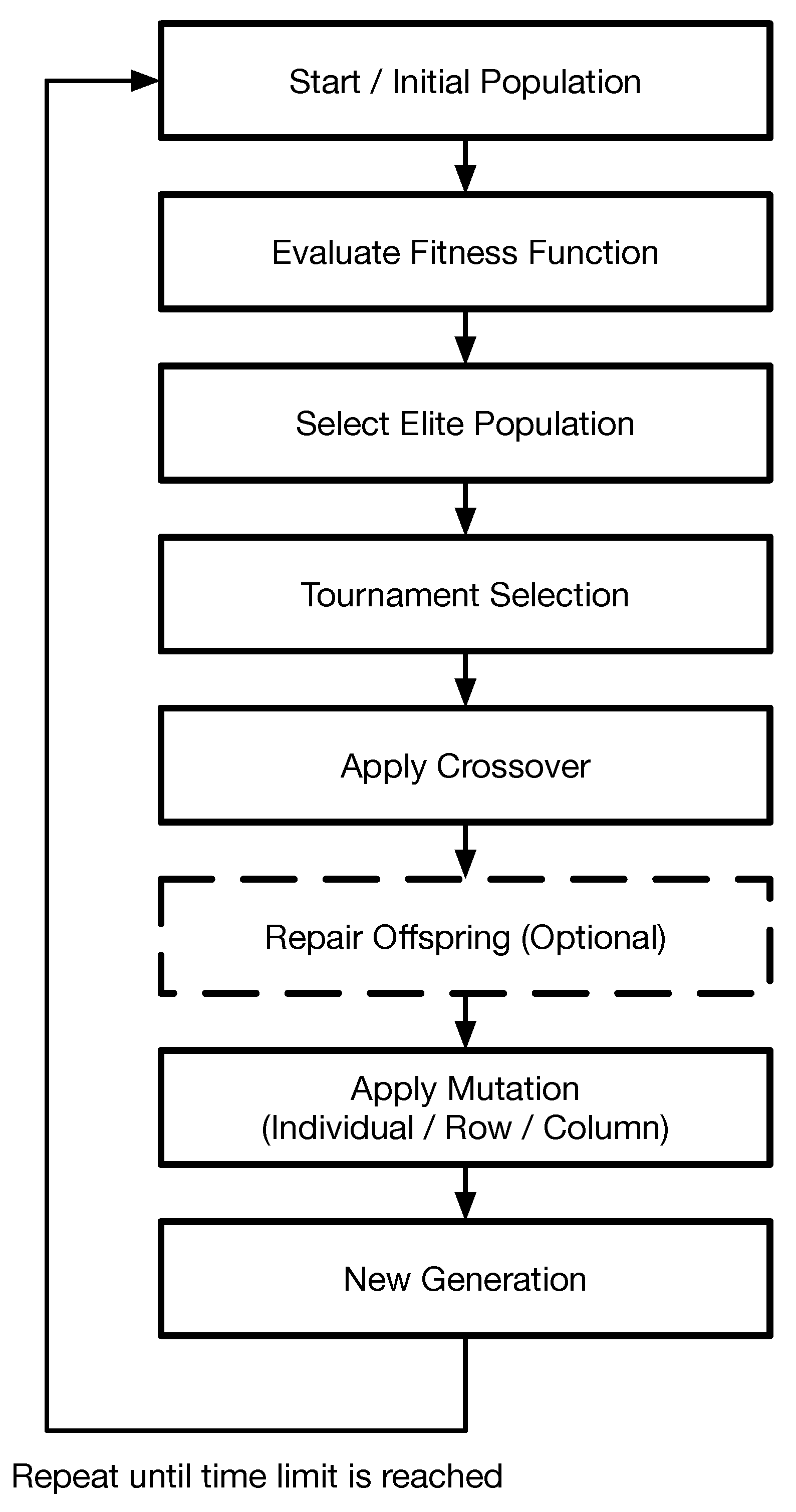
Problem (6) can also be approached by a GA, specially designed for our context. A description of the GA is shown in Algorithm 1 and Figure 2, in which five phases are considered.

Note that the feasibility of individuals is always guaranteed when crossover is employed by considering a repair algorithm. Index $j=1,\dots ,J$ is related to the time limit imposed by the GA. In essence, J can be seen as the number of generations needed during the chosen running time interval.

Algorithm 1 Genetic Algorithm (General Scheme)

1: Determine a population size POP and a time limit TL.   2: Generate initial population ${\mathbf{P}}^0$ comprising individuals ${\mathbf{C}}_1^0,\dots ,{\mathbf{C}}_{\mathrm{POP}}^0$ at random.   3: Compute fitness of each individual ${\mathbf{C}}^0\in {\mathbf{P}}^0$.   4: while Elapsed time less than TL do   5:     Perform elite population selection comprising a fraction of population ${\mathbf{P}}^j$ (optional).   6:     Perform R-way tournament selection, obtaining $\mathrm{POP}/2$ individuals of population ${\mathbf{P}}^j$.   7:     Perform crossover by selecting two individuals $({\mathbf{C}}_{\mathrm{a}}$,${\mathbf{C}}_{\mathrm{b}})\in {\mathbf{P}}^j$ at random, obtaining ${\mathbf{C}}_{\mathrm{c}}$. Such process runs POP times, with the offspring population ${\mathbf{P}}_{\mathrm{c}}^j$ consisting of POP individuals.   8:     Perform mutation over individual ${\mathbf{C}}_{\mathrm{c}}$, obtaining ${\mathbf{C}}_{\mathrm{m}}$. Such process runs POP times with the mutated population ${\mathbf{P}}_{\mathrm{m}}^j$ consisting of POP individuals.   9:     Compute fitness of each individual ${\mathbf{C}}_{\mathrm{m}}^j\in {\mathbf{P}}_{\mathrm{m}}^j$. 10: end while 11: Return the best individual among J individuals previously selected from populations ${\mathbf{P}}_{\mathrm{m}}^0,\dots ,{\mathbf{P}}_{\mathrm{m}}^J$.

5.1. Solution Structure and Initial Population

Each population is a set of POP matrices $\mathbf{C}={\left[c_{k,p}\right]}_{K\times P}$, with each matrix representing one individual. Such matrices also represent the panel allocation matrix, where $c_{k,p}\in \{0,1\}$ accounts for the activation or non-activation of panel p serving terminal k. Such matrices must satisfy Problem (6) constraints. In particular, if there are $P_{\mathrm{a}}$ active panels communicating with K terminals, matrix $\mathbf{C}$ must have $P_{\mathrm{a}}$ columns with N non-zero elements, representing the number of outputs per panel. In addition, matrix $\mathbf{C}$ must not have rows of zeros, meaning that all the terminals are being served.

If we consider a total number of panel $P=10$ with active ones $P_{\mathrm{a}}=4$, each one with $N=2$ outputs per panel and communicating with $K=4$ terminals, a valid example of an individual of a given population resulting from the use of these variables is

$$\mathbf{C}=\left[\begin{array}{cccccccccc}0& 1& 0& 0& 0& 0& 1& 0& 0& 0\\ 1& 0& 0& 0& 0& 0& 1& 1& 0& 0\\ 1& 0& 0& 0& 0& 0& 0& 1& 0& 0\\ 0& 1& 0& 0& 0& 0& 0& 0& 0& 0\end{array}\right]$$

The population will evolve during the algorithm (i.e., as the number of generations or time limit increases); however, the size of the population POP remains unchanged.

Note that the initial population is nothing more than a set of such matrices, satisfying all the constraints imposed in Problem (6).

5.2. Fitness Function

The fitness function is important to select the best individuals, determining the ability of an individual to compete with the others. The higher the fitness value, the higher the quality of the solution and the greater the chance for the individual to be reproduced in the next generation. Having our panel-based LIS, terminals must be allocated to panels in such a way that all terminals experience a reasonable QoS. In our study, we aim to jointly select $P_{\mathrm{a}}$ panels to activate and allocate them to K terminals by maximising the minimum SINR among all terminals (equivalent to maximising the minimum terminal rate). The fitness function applied to our problem is

$$\mathrm{Fitness}\mathrm{Function}=\max \left(\min \left(\sum _{p=1}^P{c}_{k,p}{\Gamma }_{k,p}\right)\right),\forall k\in \{1,\dots ,K\}$$

(7)

where $c_{k,p}\in \{0,1\}$ represents the activation or non-activation of panel p serving terminal k, and ${\Gamma }_{k,p}$ is the reported SINR per terminal for the pth panel when employing a matched filter (MF).

5.3. Elite Population

Elitism is a strategy where a limited number of individuals with the best fitness values are chosen to integrate the next generation; however, they are included in the genetic operations of selection, crossover, and mutation. Elitism prevents the random destruction caused by crossover or mutation operators of individuals with good genetics. The number of elite individuals should not be too large since it can cause excessive selective pressure and premature convergence. In essence, the $R_{\mathrm{e}}(\%)$ of the best individuals, according to the fitness function value, are selected to pass to the next generation.

5.4. Tournament Selection

The selection process uses the result of the fitness function (representing the quality of the solution) to decide whether or not an individual from the current generation will survive and be passed on to the next one. The same individual can be selected more than once. The result of the selection process is an intermediate population known as the mating pool, with size $N_{\mathrm{s}}\le \mathrm{POP}$, where a higher-quality individual has a higher probability of being selected. Operators such as crossover and mutation are then applied to some of the individuals in the mating pool.

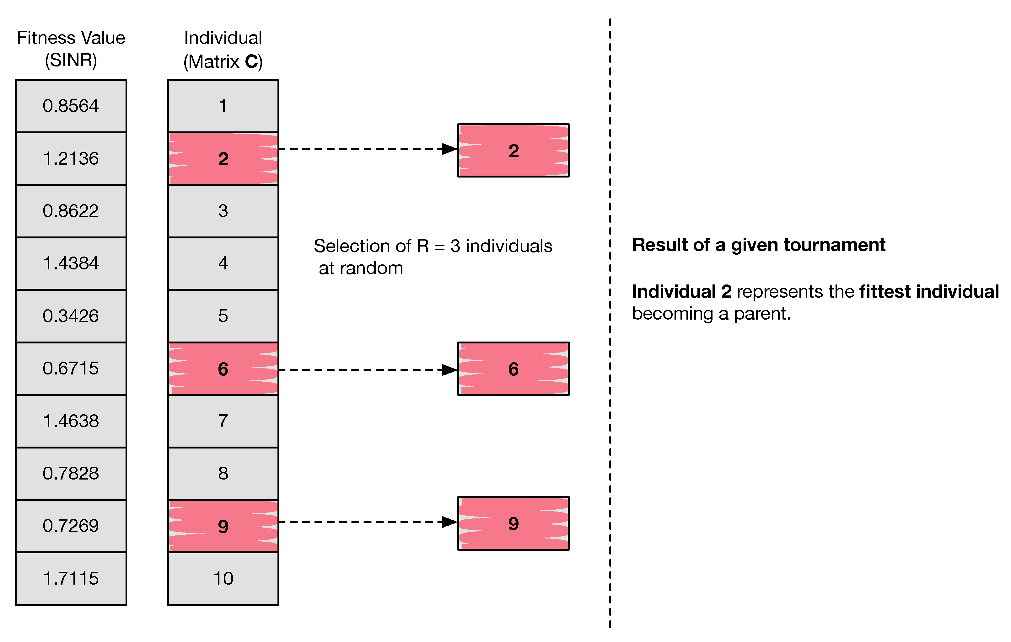
In this algorithm, we consider tournament selection. In R-way tournament selection, R individuals are selected at random, running a tournament among them afterwards. Only the fittest individual amongst the selected ones is chosen to integrate the mating pool. $N_{\mathrm{s}}$ tournaments take place, meaning that the mating pool includes $N_{\mathrm{s}}$ individuals that move on to the next genetic stages. Note that if there E elite individuals are chosen to integrate the next generation, the number of tournaments taking place is given by $N_{\mathrm{s}}=N_{\mathrm{s}}-E$. The process is described as follows and is repeated $N_{\mathrm{s}}$ times:

• Step 1: Select R individuals from the population with size POP at random.
• Step 2: Select the best out of the R individuals to become a parent.

Note that, in case the tournament size R has a large value, weak candidates have a smaller chance of getting selected. So in practice, a small tournament size is preferred, as this will maintain diversity in the population and avoid premature convergence. Figure 3 shows a simple example of one tournament selection process.

5.5. Crossover

In GAs and evolutionary computation, crossover, also called recombination, is a genetic operator that exchanges genetic information of two parents to generate new offspring. It is one way to stochastically generate new solutions from an existing population. Multiple-point crossover, uniform crossover, one-point crossover and substring crossover constitute common crossover operators. Since we are working with matrices, a column-swapping crossover operator is considered. This method changes arbitrary columns between two parents (known as individuals) to generate POP children (new individuals). The number of such columns is given by $C_{\mathrm{s}}=f_{\mathrm{s}}{P}_{\mathrm{a}}$, where $f_{\mathrm{s}}$ represents the swapping factor and P denotes the number of panels in total. Their position is chosen at random and is the same for both parents. It is important to mention that this method can easily be modified to row swapping; however, in this work, we only consider column swapping.

Let $S$ be the set of column indices referring all activated panels, of cardinality $P_{\mathrm{a}}$, for the first parent. Essentially, a number of columns are selected from set $S$ comprising all activated panels columns indexes. Such columns are then exchanged between parents, in which their position is the same for both parents. Now, assuming that there is just one column to swap, we suggest that such an index must belong to set $S$, to avoid swapping a column of zeros, so that the offspring is not identical to its parent. On the contrary, the second parent column index can be any number in the range of $[1,P]$, so either columns referring activated or non-activated panels can replace the one from parent 1. The procedure is shown in Figure 4, described as follows and repeated POP times:

• Step 1: Randomly select two parents (represented by matrices ${\mathbf{C}}_{\mathrm{a}}$ and ${\mathbf{C}}_{\mathrm{b}}$) from the population with size $N_{\mathrm{s}}$.
• Step 2: Randomly select column i, with $i\in S$.
• Step 3: Swap parents’ i-th column.
• Step 4: Repair children (if required) to become an admissible solution.

5.6. Repair Algorithm

To ensure that the constraints in Problem (6) are satisfied in the new solutions, a repair scheme is included in the crossover operator procedure. In practice, it is necessary to ensure the following points in the binary matrix $\mathbf{C}$ format:

• To have $P_{\mathrm{a}}$ columns with N non-zero values.
• To not have rows of all zeros, meaning that all terminals are being served by at least one output.

Since the columns referring to the activated panels are the only ones chosen to swap, the child matrix $\mathbf{C}$ never has more than $P_{\mathrm{a}}$ columns with N non-zero values. This means that the only case that needs to be checked is when the cardinality of set $S$ is less than $P_{\mathrm{a}}$. Now, assume a case where it is necessary to add one column with N non-zero values to complete $P_{\mathrm{a}}$ columns. Randomly, a parent (represented by matrix ${\mathbf{C}}_{\mathrm{a}}$ or ${\mathbf{C}}_{\mathrm{b}}$) is chosen to provide a column to the child that must have N non-zero values and thus belong to set $S$. Such a column will replace one of the child matrix ones related to the deactivated panels, i.e., an all-zero column. In case there is more than one panel to add, this routine is repeated for each one.

As was written previously, checking if each active panel has N outputs is equivalent to checking if each column has N non-zero elements. Due to our procedure of adding columns related to active panels to the child, such a constraint always ends up being guaranteed.

Additionally, checking if all the terminals are being served is the same as checking if the matrix $\mathbf{C}$ does not have a row of all zeros. If the reverse happens, the conflicting 0s are replaced by carefully selected positions of 1s. Now, assume a case where there is one all-zero row in the child matrix $\mathbf{C}$. From the same matrix, a column regarding active panels is chosen at random. From such a column, one of the N non-zero values is selected to replace the 0 value in the all-zero row and in the same column position. The 1 value from the old row is then deleted. In case there is more than one row to repair, this routine is repeated until there are none to repair. The procedure is shown in Figure 5.

5.7. Mutation

Mutation is a genetic operator used to maintain the genetic diversity of a population of individuals between generations. In particular, such an operator randomly changes a part of the offspring population resulting from the crossover stage. In our case, mutation can be performed by exchanging a number of randomly chosen columns or rows (also called horizontal array mutation and vertical array mutation, respectively) using a given mutation rate. Two mutation techniques can be adopted:

• Mutation per individual.
• Mutation per row or column.

In both cases, there is always the possibility of swapping either columns or rows, differing only in the approach, taking into account the probability of mutation. The probability of mutation is usually chosen as a very small number; otherwise, the algorithm may become a random search.

5.7.1. Mutation per Individual

For a given population and for each individual, a random number $r\in [0,1]$ is generated. If $P_{\mathrm{m}}$ is the probability of mutation, in case $r<P_{\mathrm{m}}$, an individual will be mutated. This operator assigns mutation probability $P_{\mathrm{m}}$ with which an arbitrary individual in a population is changed. This process is described as follows, where the steps are carried out per individual selected to be mutated:

• Step 1: Generate a random $r\in [0,1]$.
• Step 2: With a given population comprising POP individuals, if $r<P_m$, column or row mutation is performed in a given individual; otherwise, the individual is kept fixed for the next generation.
• Step 3: Generate a random $v\in \{1,2\}$. If $v=1$, row-wise mutation is performed (Step 4); otherwise, column-wise mutation is performed (Step 5).
• Step 4 (row-wise mutation): Assume there are $N_{\mathrm{r}}$ rows to exchange within a given individual, with $N_{\mathrm{r}}$ being given by the same number for all individuals to be mutated. For each row, perform the next steps. Generate two random integers $r_1,r_2\in [1,K]$, with $r_1\ne r_2$. Rows $r_1$ and $r_2$ are then exchanged in matrix $\mathbf{C}$.
• Step 5 (column-wise mutation): Assume there are $N_{\mathrm{c}}$ columns to exchange within a given individual, with $N_{\mathrm{c}}$ also being given by the same number for all individuals to be mutated. For each column, perform the next steps. Generate two random integers $c_1,c_2\in [1,P]$, with $c_1\ne c_2$. Columns $c_1$ and $c_2$ are exchanged in matrix $\mathbf{C}$.

Although the probability of mutation should be a very small number, in our case, since we are treating it as a process happening per individual, the probability should be higher to ensure that at least one individual is mutated. Setting $P_{\mathrm{m}}$ as a very small value leads to a decrease in the diversity to just a few individuals, and sometimes, anyone is selected to be mutated. This statement is properly explained in the Performance Results Section.

5.7.2. Mutation per Row or Column

For a given population and a given individual, a random number $r\in [0,1]$ is generated for all rows or all columns, depending if a row-wise or column-wise mutation approach is being considered. If $r<P_{\mathrm{m}}$, a number of rows or columns will be mutated. In essence, mutation is performed within an individual, namely using the mutation probability to pick which rows or columns should be swapped. In comparison with the previous method, the number of columns or rows to swap (and if there are columns or rows to be swapped because there is the possibility of none of them being swapped) is decided by condition $r<P_{\mathrm{m}}$. The process is described as follows, whose next steps are performed per individual, which, in this case, are POP individuals:

• Step 1: Generate a random $v\in \{1,2\}$. If $v=1$, row-wise mutation is performed (Step 2); otherwise, column-wise mutation is performed (Step 3).
• Step 2 (row-wise mutation): Generate a random $r\in [0,1]$ for each row. For rows verifying $r<P_m$, a row-wise mutation is performed. Such rows are swapped with the remaining ones satisfying $r>P_m$. Note that the number of rows to swap is entirely decided by constraint $r<P_m$. It is possible to have a case where there are no rows to exchange. The swapping process is similar to the one described for mutation per individual.
• Step 3 (column-wise mutation): Generate a random $r\in [0,1]$ for each column. For columns verifying $r<P_m$, a column-wise mutation is performed. Such columns are swapped with the remaining ones satisfying $r>P_m$. The swapping process is similar to the one described for mutation per individual.

In this case, a low mutation probability provides enough diversity because it is performed within an individual, using its rows or columns for this purpose. Therefore, this method is capable of introducing new individuals to be included in the next generation, perhaps leading to an overall better solution at the end. This statement is properly explained in the Performance Results Section. Since all changes imposed by the mutation operator are carried out within matrix $\mathbf{C}$ (i.e., within a given individual), mainly by swapping entire rows and columns, solution admissibility is always guaranteed.

Figure 6 shows a simple example showing the column-wise approach that can happen in both mentioned mutation techniques. In case it is a mutation per individual, the individuals with $r<P_m$ are picked to be mutated, with the number of columns/rows being set manually. If it is a mutation per column/row, such a process is applied in each individual and in rows/columns satisfying $r<P_m$. In essence, the swapping stage is similar for both mutation operators; however, the steps taken before are different.

6. Performance Results

This section presents the performance results for the GA designed for the joint panel selection and terminal association problem.

Table 1. Problem Variables Description.

Variables	Description
POP	Population size
$R_{\mathrm{e}}$	Elite rate (percentage of population to integrate into next generation)
$N_{\mathrm{s}}$	Number of individuals selected for crossover and mutation processes
$C_{\mathrm{s}}$	Number of columns to be swapped between parents in crossover
$f_{\mathrm{s}}$	Swapping factor to be used in $C_{\mathrm{s}}$ expression
r	Random number in range [0, 1]
$P_m$	Mutation rate in range [0, 1]
v	Random number from group {1,2}
$N_{\mathrm{r}}$	Number of rows to exchange within an individual (mutation per individual)
$N_{\mathrm{c}}$	Number of columns to exchange within an individual (mutation per individual)
TL	Time limit
$\mathbf{C}$	Matrix representing an individual with size $K\times P$
P	Number of activated and non-activated panels
	Number of columns in matrix $\mathbf{C}$
$P_{\mathrm{a}}$	Number of activated panels
	Number of columns in matrix $\mathbf{C}$ with non-zero values
N	Number of outputs per panel
	Number of non-zero elements in each column from group of $P_{\mathrm{a}}$ ones in matrix $\mathbf{C}$

presents a brief description of each parameter used in the GA, and it is important to interpret the results.

In terms of the scenario, we consider a rectangular room, in which the LIS, with a total area of 36 m², is located on the ceiling, as shown in Figure 1. This configuration represents a realistic and representative configuration for panel-based LIS deployment and was selected to reflect typical physical constraints and dimensions found in practical applications, such as indoor environments.

This surface is located at $0\le x\le 18$ and $0\le y\le 2$ and $z=2.5$, whose panels are square and contiguous, presenting an identical area. Considering that the LIS total area, B, is fixed, for different values of $\tau$ and $A_{\mathrm{p}}$, the number of panels is calculated by the following:

$$P_a={\displaystyle \frac{\tau B}{A_p}}.$$

(8)

In our case, we consider a scenario where $40\%$ of the total LIS area is activated ($\tau =40\%$), comprising panels with an area $A_{\mathrm{p}}=0.2$ m². Each panel contains $N=6$ outputs per panel. The number of total panels is given by $P=160$ and the number of activated ones is $P_{\mathrm{a}}=73$. We assume that terminals are distributed within the room area according to the Poisson process, whose intensity is given by ${\lambda }_{\mathrm{K}}=1$ m². Furthermore, we assume unitary transmitted power per terminal and a noise density of $N_0={10}^{-4}$ (W/Hz), with our results shown for MF equalisation.

Our investigation was conducted with population size $\mathrm{POP}=40$ and TL was set to $\{600,1800,3600\}$ s. In all simulations, tournament selection is considered, in which the number of individuals to be picked randomly, R, is $10\%$ of population size POP, which is 4. The R-way tournament selection procedure is repeated $\mathrm{POP}/2$, meaning that only half of the initial population is selected for crossover and mutation, with $N_{\mathrm{s}}=20$. Regarding the crossover operator, swapping factor $f_{\mathrm{s}}$ is set to $\{0.2,0.5,0.8\}$, with the number of columns to swap between parents being given by $C_{\mathrm{s}}=f_{\mathrm{s}}{P}_{\mathrm{a}}\in \{15,37,58\}$. Two different mutation operators are taken into consideration, mutation per individual and mutation per row/column, with mutation rate $P_{\mathrm{m}}\in \{0.05,0.3\}$. In case mutation per individual is applied, constraint $r<P_{\mathrm{m}}$ only decides which individuals will be mutated. Similarly to the crossover operator, swapping factor $f_{\mathrm{s}}$ is set to $\{0.2,0.5,0.8\}$, with the number of rows or columns to swap within an individual being given by $N_{\mathrm{r}}=f_{\mathrm{s}}{P}_{\mathrm{a}}\in \{8,20,31\}$ or $N_{\mathrm{c}}=f_{\mathrm{s}}{P}_{\mathrm{a}}\in \{15,37,58\}$, respectively. If mutation per row/column is considered, the number of rows/columns is entirely decided by the constraint $r<P_{\mathrm{m}}$, which is not set manually. Finally, elitism is used in some simulations aiming at preventing the random destruction caused by crossover or mutation operators of some important individuals. In our case, only the $R_{\mathrm{e}}=5\%$ of the best individuals are selected to pass directly to the next generation, thus having $E=2$ individuals in this condition. Even though they pass directly to the next generation, they are still used for crossover and mutation purposes, having an important role in the convergence of the algorithm. The GA ran ten times for each case and exactly followed the structure of Algorithm 1. The stopping criterion for the GA was a fixed time limit, corresponding to a maximum number of generations within that time, as our objective was to assess its performance against the CPLEX solver to evaluate the trade-offs in solution quality and time computational efficiency. The GA and the CPLEX solver were executed on the same system under identical conditions. The experiments were conducted on a machine equipped with Intel(R) Xeon(R) Silver 4110 CPU @ 2.10GHz (Intel Corporation, Santa Clara, CA, USA), with eight cores, 16 threads and 64 GB RAM, running Ubuntu 18.04.6 LTS.

6.1. Mutation per Individual Versus Mutation per Row/Column

Figure 7, Figure 8 and Figure 9 represent the GA evolution along 600 s (10 min), employing mutation per individual and a crossover operator both with $f_{\mathrm{s}}\in \{0.2,0.5,0.8\}$, respectively, considering the mutation rate $P_{\mathrm{m}}=0.3$. The main difference between Figure 7, Figure 8 and Figure 9 lies in the swapping factor, $f_s$, used during the crossover operation. Each figure presents results for both elitist and non-elitist populations. A quantitative analysis of these results is provided in

Table 2. Comparative results for 10 runs considering $P_{\mathrm{m}}=0.3$ and $f_{\mathrm{s}}\in \{0.2,0.5,0.8\}$ for a $\mathrm{TL}=600$ s. Depending on which option is selected while performing crossover operation, $N_{\mathrm{r}}\in \{8,20,31\}$ rows and $N_{\mathrm{c}}\in \{15,37,58\}$ columns are randomly chosen to swap. This table represents cases in Figure 7, Figure 8 and Figure 9.

Case Setting	Best	Mean	Worst	Median	STD	IQR
No Elitism ($f_{\mathrm{s}}=0.2$)	3.9259	3.7864	3.5956	3.8071	0.1007	0.1185
Elitism ($f_{\mathrm{s}}=0.2$)	3.7813	3.6760	3.5851	3.6536	0.0704	0.1260
No Elitism ($f_{\mathrm{s}}=0.5$)	3.4499	3.2584	3.0530	3.2863	0.1298	0.1946
Elitism ($f_{\mathrm{s}}=0.5$)	3.2602	3.1086	2.9976	3.0898	0.0982	0.1409
No Elitism ($f_{\mathrm{s}}=0.8$)	3.3042	3.0763	2.826	3.098	0.1397	0.1773
Elitism ($f_{\mathrm{s}}=0.8$)	3.1059	2.9513	2.7592	2.9806	0.1143	0.1368

.

In all cases, the use of elitism does not represent a decisive factor for achieving a better solution, which in our case is the minimum SINR. So in some cases, having elitism does not mean achieving a better solution along the algorithm running time, as shown also in Table 2 for 10 runs. Furthermore, the performance results employing elitism and not employing it are similar, including in the low diversity created by crossover and mutation operators. Regarding the $f_{\mathrm{s}}$ parameter, considering higher values, meaning more changes during crossover and mutation, leads to the random destruction of solutions, proven in Table 2, showing no improvement in the best solution as $f_{\mathrm{s}}$ increases.

Figure 10 only differs from Figure 7 in the value of $P_{\mathrm{m}}=0.05$. By comparing these figures, it is observed that the only way to provide some diversity is to increase mutation rate $P_{\mathrm{m}}$, even though such diversity is not that high. Increasing mutation rate $P_{\mathrm{m}}$ increases the probability of having more individuals mutated. With small mutation rates, there is not even a gap between the fitness function average value and fitness value related to the best solution in each generation within the considered time limit, showing the non-existence of diversity.

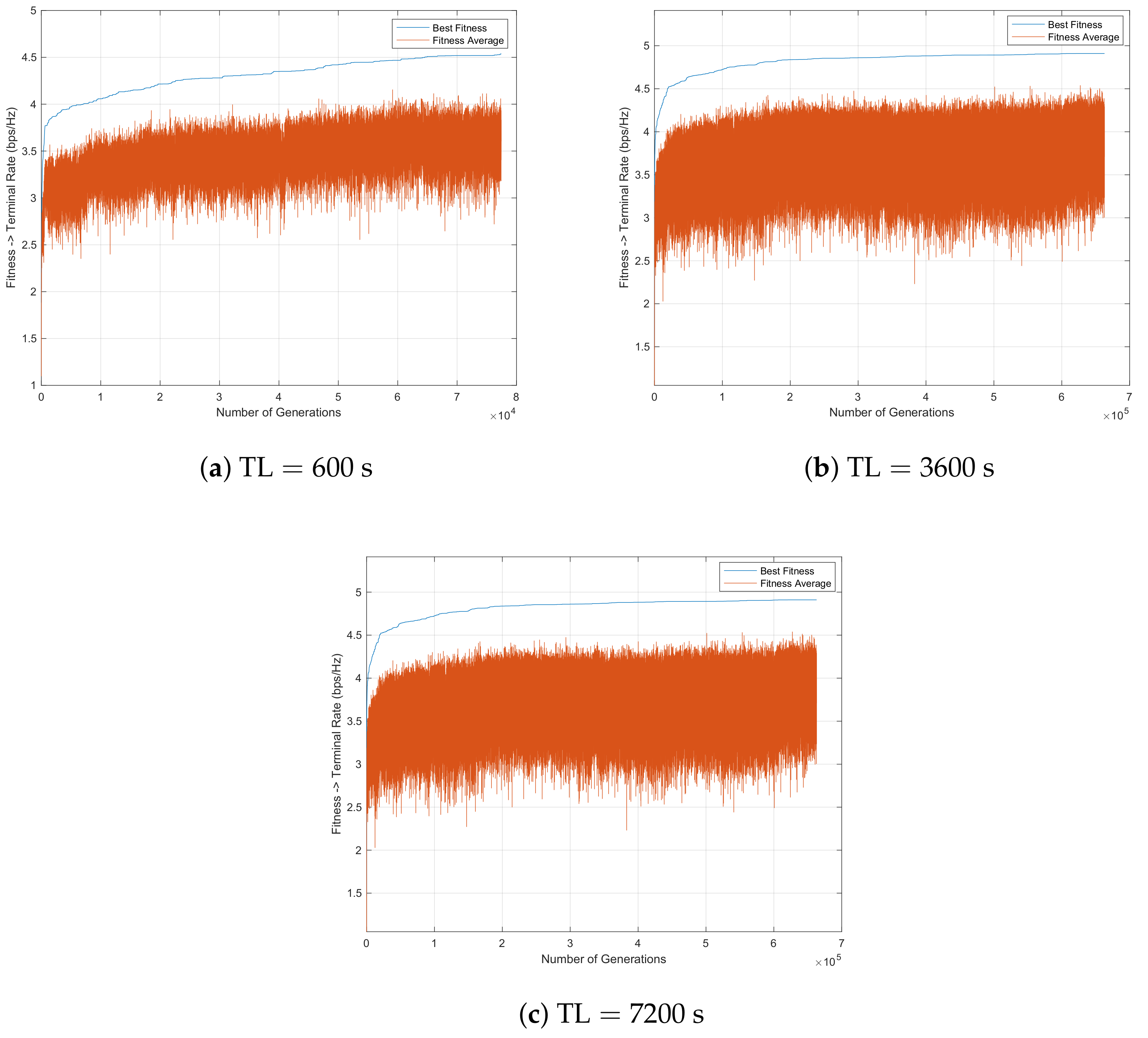
Figure 11 and Figure 12 represent the GA evolution along $\{600,3600,7200\}$ s, employing mutation per row/column with $P_{\mathrm{m}}=0.05$. For both cases, the use of elitism enables a better solution in the end. Moreover, the introduction of diversity is not due to the fact of including elitism or not. It seems that the crossover and mutation operators are sufficient to introduce a high level of diversity, contributing significantly to the achievement of a good solution, especially for the case where elitism is used, as can be seen in

Table 3. Comparative results for 10 runs considering $P_{\mathrm{m}}=0.05$ and $f_{\mathrm{s}}=0.2$ for crossover operator for $\mathrm{TL}=600$ s. This table represents the case in Figure 11.

Case Setting	Best	Mean	Worst	Median	STD	IQR
No Elitism	2.9814	2.9282	2.8747	2.9334	0.0335	0.0415
Elitism	4.5229	4.4347	4.3718	4.4490	0.0468	0.0670

. In this case, small mutation rates no longer sacrifice the diversity factor. Furthermore, since mutation per row/column is carried out within the individual, determining which rows/columns are chosen to be exchanged using the mutation rate for this purpose, more modifications are likely to happen. As expected, as the time limit increases, this is the best solution.

As seen in Figure 11 and Table 3, the best solution is achieved when parameters such as elitism and mutation per column/row are considered. For this reason, this scenario is chosen to be compared with the CPLEX solver. Furthermore,

Table 4. Comparative results for 10 runs considering elitism of $E=2$ individuals, $f_{\mathrm{s}}=0.2$ for crossover operator and $P_{\mathrm{m}}=0.0025$, for $\mathrm{TL}\in \{600,3600,7200\}$ s.

TL (s)	Best	Mean	Worst	Median	STD	IQR
600	4.7941	4.6158	4.5084	4.6119	0.0866	0.1243
3600	4.8808	4.8322	4.7529	4.8380	0.0411	0.0429
7200	4.9359	4.8983	4.8433	4.9074	0.0315	0.0511

shows that an increase in the time limit enables a general improvement in the descriptive statistic values.

6.2. Mutation per Row/Column Considering Elitism Versus CPLEX Solver

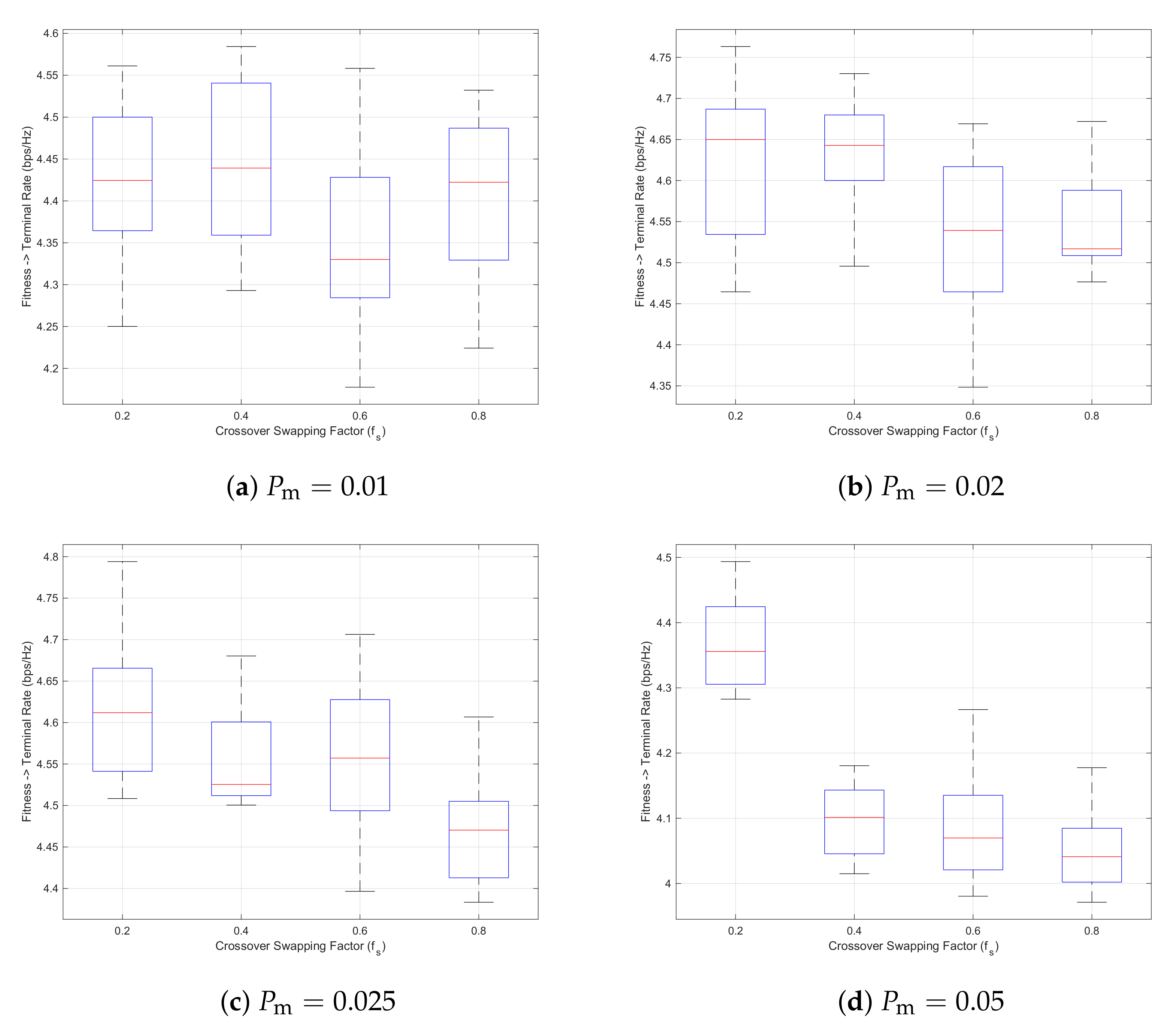
With the purpose of obtaining the best solution possible, several experiments are conducted for different parameter combinations of $P_{\mathrm{m}}$ and $f_{\mathrm{s}}$. Each case is represented in

Table 5. Comparative results for 10 runs considering $P_{\mathrm{m}}\in \{0.01,0.02,0.025,0.05\}$ and $f_{\mathrm{s}}\in \{0.2,0.4,0.6,0.8\}$ for a $\mathrm{TL}=600$ s. Depending on which option is selected while performing the crossover operation, $C_{\mathrm{s}}\in \{15,29,44,58\}$ columns are randomly chosen to swap. This table represents cases in Figure 13.

Elitism	Best	Mean	Worst	Median	STD	IQR
$P_{\mathrm{m}}=0.01$ | $f_{\mathrm{s}}=0.2$	4.5611	4.4260	4.2501	4.4244	0.0934	0.1356
$P_{\mathrm{m}}=0.01$ | $f_{\mathrm{s}}=0.4$	4.5843	4.4446	4.2929	4.4392	0.0989	0.1816
$P_{\mathrm{m}}=0.01$ | $f_{\mathrm{s}}=0.6$	4.5583	4.1775	4.3540	4.3300	0.1150	0.1438
$P_{\mathrm{m}}=0.01$ | $f_{\mathrm{s}}=0.8$	4.5322	4.4070	4.2242	4.4223	0.1008	0.1575
$P_{\mathrm{m}}=0.02$ | $f_{\mathrm{s}}=0.2$	4.7632	4.6212	4.4645	4.6500	0.0983	0.1526
$P_{\mathrm{m}}=0.02$ | $f_{\mathrm{s}}=0.4$	4.7302	4.6332	4.4957	4.6428	0.0672	0.0798
$P_{\mathrm{m}}=0.02$ | $f_{\mathrm{s}}=0.6$	4.6692	4.5351	4.3484	4.5393	0.1046	0.1524
$P_{\mathrm{m}}=0.02$ | $f_{\mathrm{s}}=0.8$	4.6720	4.5491	4.4766	4.5169	0.0673	0.0795
$P_{\mathrm{m}}=0.025$ | $f_{\mathrm{s}}=0.2$	4.7941	4.6158	4.5084	4.6119	0.0866	0.1243
$P_{\mathrm{m}}=0.025$ | $f_{\mathrm{s}}=0.4$	4.6803	4.5599	4.5005	4.5254	0.0663	0.0889
$P_{\mathrm{m}}=0.025$ | $f_{\mathrm{s}}=0.6$	4.7063	4.5605	4.3965	4.5572	0.1047	0.1340
$P_{\mathrm{m}}=0.025$ | $f_{\mathrm{s}}=0.8$	4.6068	4.4726	4.3834	4.4704	0.0738	0.0922
$P_{\mathrm{m}}=0.05$ | $f_{\mathrm{s}}=0.2$	4.4936	4.3651	4.2826	4.3558	0.0676	0.1190
$P_{\mathrm{m}}=0.05$ | $f_{\mathrm{s}}=0.4$	4.1806	4.0997	4.0150	4.1014	0.0551	0.0977
$P_{\mathrm{m}}=0.05$ | $f_{\mathrm{s}}=0.6$	4.2667	4.0949	3.9805	4.0697	0.0981	0.1144
$P_{\mathrm{m}}=0.05$ | $f_{\mathrm{s}}=0.8$	4.1776	4.0500	3.9712	4.0411	0.0656	0.0826

(we note that no advanced statistical tests were applied to assess the significance of differences between parameter configurations, as the observed variability across configurations was minimal), also defined by a box plot. In this case, a range bar is drawn to represent the interquartile range (IQR) of the data set, which indicates the degree of dispersion in a data set. The median value is identified with a red line, and the ends of the whiskers stand for the minimum and maximum values, respectively. Overall, the best parameter combination is the case considering $P_{\mathrm{m}}=0.025$ and $f_{\mathrm{s}}=0.02$. This scenario will be compared with the solution when using the CPLEX solver.

Figure 13. GA solution distribution considering random crossover and mutation per row/column with swapping factor $f_{\mathrm{s}}\in \{0.2,0.4,0.6,0.8\}$ with $P_{\mathrm{m}}\in \{0.01,0.02,0.025,0.05\}$ during $\mathrm{TL}=600$ s for 10 runs.

Figure 13. GA solution distribution considering random crossover and mutation per row/column with swapping factor $f_{\mathrm{s}}\in \{0.2,0.4,0.6,0.8\}$ with $P_{\mathrm{m}}\in \{0.01,0.02,0.025,0.05\}$ during $\mathrm{TL}=600$ s for 10 runs.

Table 6. CPLEX vs. GA using elitism of $E=2$ individuals, $f_{\mathrm{s}}=0.2$ for crossover operator and mutation per row/column with $P_{\mathrm{m}}=0.025$, for $\mathrm{TL}\in \{30,60,90,120,150,240,600,3600,7200\}$ s and 10 independent runs. CPLEX solution is compared with ones from Figure 12. % gap is relative difference between best solution and best known bound for solution.

TL		30	60	90	120	150	240	600	3600	7200
CPLEX Solver	SINR (bits/s/Hz)						4.9835
	Performance Loss (%)						0.02
Genetic Algorithm	SINR (bits/s/Hz)	4.0449	4.1946	4.2693	4.3272	4.3715	4.4556	4.7941	4.8808	4.9359
	Performance Loss (%)	18.85	15.84	14.35	13.19	12.30	10.61	3.82	2.08	0.98
	Avg. Number of Generations	3310	6753	10,234	13,561	16,826	26,823	66,093	39,9321	796,119

compares the best GA solution with the one achieved by running the CPLEX solver for different time constraints. The best solution is selected from a group of 10 solutions resulting from the same number of independent runs.

It is observed that the CPLEX solver is able to provide a feasible integer solution within $0.02\%$ of the optimal, which is extremely close to the optimum value (the default gap is $0.01\%$ in CPLEX). This feasible integer solution is used for comparison. The GA algorithm runs for $\mathrm{TL}\in \{30, 60, 90, 120, 150, 240, 600, 3600, 7200\}$ s, achieving a solution $\{18.85, 15.84, 14.35, 13.19, 12.30, 10.61, 3.82, 2.08, 0.98\}$% lower than the one achieved in the CPLEX solver, respectively. Although mutation per column/row is able to provide higher diversity (enabling the GA algorithm to evolve successfully), the CPLEX solver continues to deliver better solutions (i.e., higher max–min terminal rates) in comparison with the proposed GA algorithm. However, Table 6 shows that, while the CPLEX solver converges to a feasible solution after 240 s (with an optimality gap of $0.02\%$), the proposed GA algorithm is still capable of providing acceptable solutions in less running time (i.e., 60 to 120 s). In fact, the solutions provided by the proposed GA algorithm yields performance losses ranging from 18.85 to 12.30% (in comparison with the feasible integer solution provided by the CPLEX solver), making the proposed GA algorithm particularly attractive for scenarios where faster approximations are preferred over exact solutions. Therefore, the proposed GA is capable of delivering satisfactory solutions in a faster manner without the need for extensive computational resources. Based on a linear interpolation of the results, the number of generations required to reach 95% of the optimal fitness (i.e., $\mathrm{SINR}=4.7353$) is approximately 59,268 generations. Furthermore, the convergence can be empirically verified in Table 6 as the number of generations increases because when the stopping condition (i.e., the time limit or maximum number of generations) is increased, the SINR solution obtained by the GA also improves progressively. This indicates that the GA continues to refine the solution and move closer to the optimum as more generations are allowed.

On the whole, both the CPLEX solver and the GA algorithm can be viable options to solve Problem (6). In particular, the CPLEX solver is a viable option when more accurate (e.g., exact) solutions are required, whereas the GA algorithm is a viable option when faster and consequently less accurate solutions are preferred over exact solutions.

7. Conclusions

In this paper, we propose a GA for panel selection and panel–terminal association for panel-based LIS architectures. This algorithm aims at allocating a set of terminals to a given panel, the panel comprising a limited number of baseband outputs, while maximising the minimum SINR.

It is shown that, although the CPLEX solver obtains superior solutions (i.e., superior max–min terminal rates) within the given time limits, the proposed GA algorithm can still provide acceptable solutions in a faster and consistent manner across shorter time limits, with such acceptable solutions yielding performance losses ranging from 18.85 to 12.30% (in comparison with the feasible integer solution provided by the CPLEX solver). The delivery of such acceptable solutions demonstrates the ability of the GA algorithm to perform a robust search of solutions while ensuring scalability (as there is no need for extensive computational resources).

While the proposed GA demonstrates the ability to produce acceptable solutions within a limited computational time, it may not always converge to a near-optimal solution, particularly in more complex scenarios. Furthermore, extending the method to support dynamic or real-time scenarios, where constraints or inputs evolve over time, represents a promising but difficult direction. In such cases, hybrid approaches, such as combining the GA with a more localised search or machine learning [33,34], could help improve convergence and solution quality.