Machine Learning-Based Predictive Model for Risk Stratification of Multiple Myeloma from Monoclonal Gammopathy of Undetermined Significance

Abstract

Monoclonal Gammopathy of Undetermined Significance (MGUS) is a precursor to hematologic malignancies such as Multiple Myeloma (MM) and Waldenström Macroglobulinemia (WM). Accurate risk stratification of MGUS patients remains a clinical and computational challenge, with existing models often misclassifying both high-risk and low-risk individuals, leading to inefficient healthcare resource allocation. This study presents a machine learning (ML)-based approach for early prediction of MM/WM progression, using routinely collected hematological data, which are selected based on clinical relevance. A retrospective cohort of 292 MGUS patients, including 7 who progressed to malignancy, was analyzed. For each patient, a feature descriptor was constructed incorporating the latest biomarker values, their temporal trends over the previous year, age, and immunoglobulin subtype. To address the inherent class imbalance, data augmentation techniques were applied. Multiple ML classifiers were evaluated, with the Support Vector Machine (SVM) achieving the highest performance (94.3% accuracy and F1-score). The model demonstrates that a compact set of clinically relevant features can yield robust predictive performance. These findings highlight the potential of ML-driven decision-support systems in electronic health applications, offering a scalable solution for improving MGUS risk stratification, optimizing clinical workflows, and enabling earlier interventions.

1. Introduction

Monoclonal gammopathies encompass a spectrum of diseases characterized by the proliferation of clonal B or plasma cell disorders. These diseases range from benign conditions, such as Monoclonal Gammopathy of Uncertain Significance (MGUS), to malignant conditions, including Multiple Myeloma (MM) or Waldenström Macroglobulinemia (WM) [1].

MGUS is an asymptomatic condition defined by the presence of a serum monoclonal M-Protein level below 3 g/dL or an abnormal serum free light chain (FLC) ratio <100, and, if a bone marrow study (BMS) is performed, bone marrow plasma cell involvement must be <10% [2,3]. Although MGUS is benign, it carries a risk of progression to a malignant disorder, with an estimated annual rate of 0.5–1%. This progression risk is not constant for individual patients and can fluctuate, necessitating indefinite follow-up with at least annual laboratory testing. Furthermore, the interval from MGUS to the development of MM or MW can range from 1 to 32 years [4,5,6,7]. This prolonged and variable course, coupled with the need for ongoing monitoring, creates considerable temporal and economic burdens on healthcare systems, which are further amplified by an aging global population.

Risk stratification aims to identify patients with a higher probability of disease progression who consequently require more intensive monitoring. In contrast, early diagnosis involves confirming active malignancy through diagnostic procedures, such as bone marrow biopsy or imaging. These procedures are associated with significant costs and can cause physical or psychological distress to patients, underscoring the need for more precise risk stratification tools.

Artificial Intelligence (AI), particularly its subfield Machine Learning (ML), is increasingly being applied across various healthcare domains [8,9,10]. ML algorithms learn from data by identifying complex patterns without being explicitly programmed with predefined rules [11,12,13]. In this manner, ML models can discern patterns in the health trajectories of large patient cohorts [14,15,16]. Within hematology, ML has been successfully employed for predictive modeling tasks, including blood cell classification [17], acute myeloid leukemia diagnosis [18], and classification of lymphoma subtypes [19]. These applications highlight the potential of ML to improve clinical decision-making in complex hematological disorders. However, to our knowledge, few ML models have been developed for MGUS risk stratification using routine, longitudinal laboratory data. Addressing this gap could facilitate the development of more accurate and personalized management strategies for patients with MGUS.

Based on these considerations, we hypothesize that analyzing routine blood test results with a machine learning-based model can enhance risk stratification. This could enable timely intervention for high-risk MGUS patients and potentially reduce monitoring intensity for those at low risk. For this purpose, we conducted a retrospective observational analysis of MGUS patients to perform an exhaustive evaluation of various ML classifiers for predicting progression to MM/WM and to identify biological indicators most strongly associated with malignant development.

The rest of the manuscript is structured as follows. In Section 2, related work is explored. Section 3 presents the tools and methods used in this paper. Next, Section 4 describes the experimental section. In Section 5, the results obtained in the experiments are discussed, as well as the clinical applications of the proposed solution. Finally, conclusions and future work are listed in Section 6.

2. Related Work

2.1. Risk Stratification

Current risk stratification models, exemplified by the Mayo Clinic risk score, rely on a limited number of factors (e.g., M-protein size, serum FLC ratio, and presence of abnormal immunoparesis) and may not fully encompass the complex dynamics of MGUS progression [2,20]. Consequently, these models can lead to over- or under-estimation of individual risk, resulting in suboptimal resource allocation and increased patient anxiety [21]. Notably, these models typically do not integrate temporal changes in key biomarkers or consider the potential interdependencies among various laboratory parameters [22]. Longitudinal monitoring of trends, rather than static values, is also gaining recognition as a more accurate predictor of malignant transformation. Recently, machine learning-based models have shown promising accuracy in predicting progression from MGUS to multiple myeloma by integrating high-dimensional immunological, epigenetic, and laboratory features [20].

2.2. Data Augmentation

Data augmentation is a common technique in AI, particularly for scarce or imbalanced datasets. It involves generating synthetic data instances by introducing minor variations to existing data, thereby increasing dataset diversity and volume. This technique is frequently employed in clinical applications, such as medical imaging and early diagnosis [23,24].

2.3. Machine Learning Comparative Studies

In the past decade, several authors conducted exhaustive analyses of machine learning algorithms for disease diagnosis and prediction, including general studies [25,26] or disease-specific studies, such as skin cancer [27] or breast cancer [28]. However, these studies focused on medical imaging and not on blood test results. In the present paper, we perform a comprehensive evaluation of ML models for risk stratification of MGUS patients, which are trained with biological indicators extracted from routine blood tests.

3. Methodology

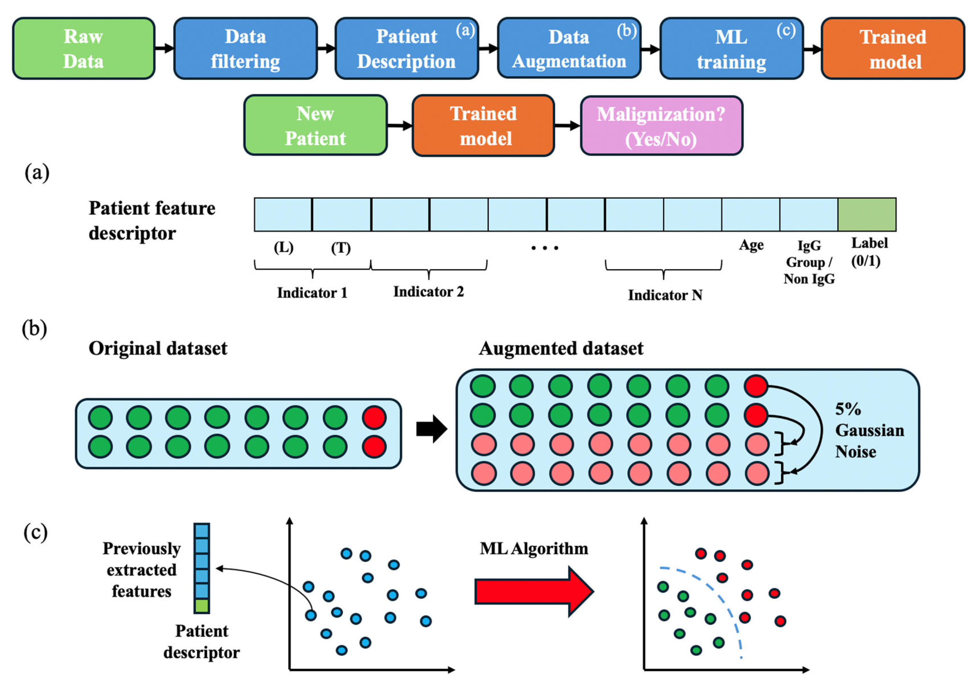
Figure 1 presents an overview of the methodology employed in this study, which is detailed in the following subsections.

3.1. Study Setting and Population

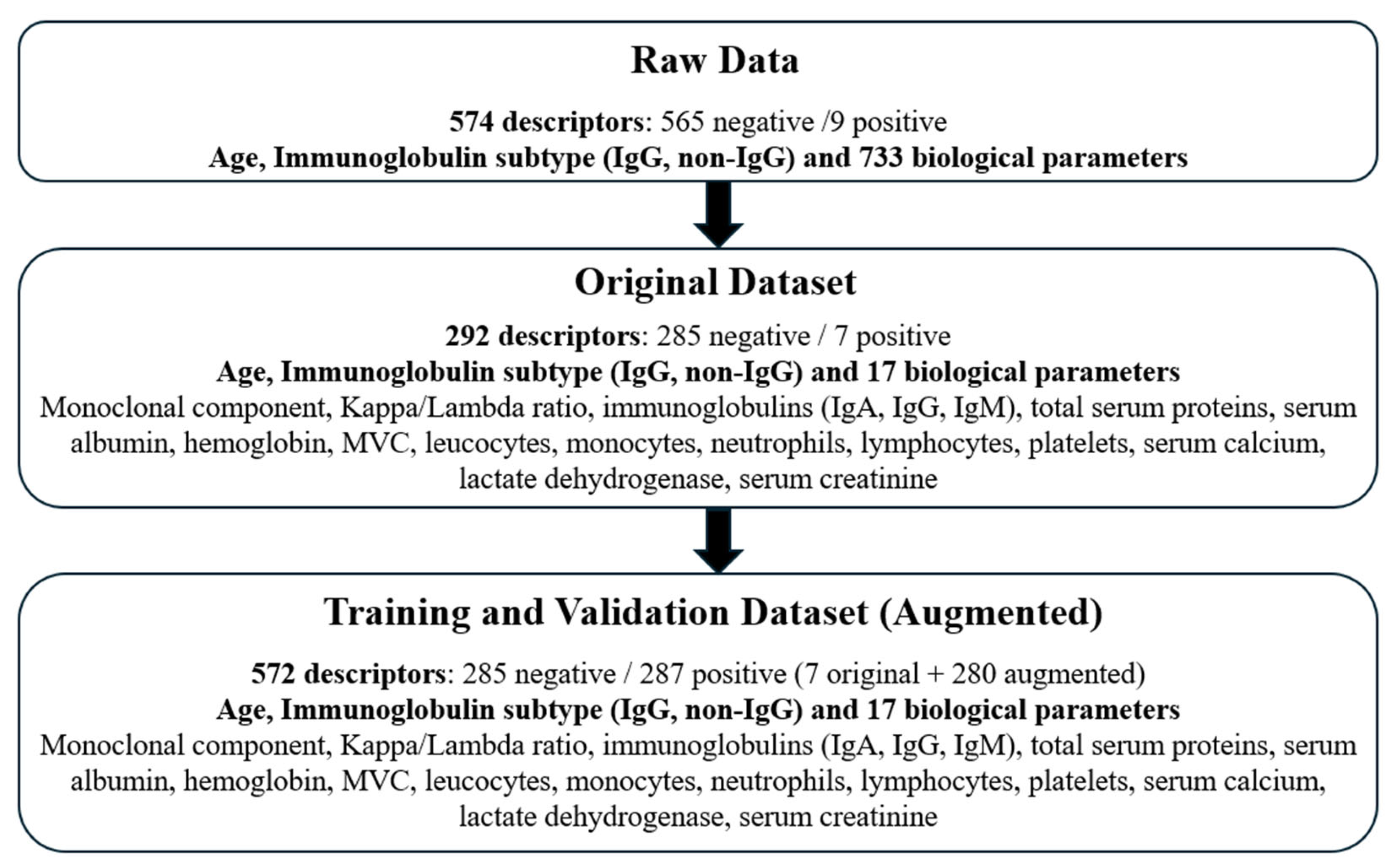
This retrospective study utilized anonymized data from patients diagnosed with MGUS at University Vinalopó Hospital (UVH) between 1 January 2010 and 31 December 2023. For each patient, we collected blood test results and MM/WM diagnostic information according to the International Myeloma Working Group Criteria 2010 and 2014 [2,3]. The initial dataset comprised 574 patients, encompassing a total of 23,314 blood tests. The study was conducted in accordance with the Declaration of Helsinki, and the protocol was approved by the Ethics Committee of the UVH in January 2023 (Project identification code 2022_063). Informed consent was not required due to the retrospective design and use of pseudonymized data.

3.2. Data Filtration and Preparation

Initially, we extracted data for 733 biological parameters from all available laboratory blood tests. Based on biological relevance and frequency of measurement, we selected 17 key parameters. These parameters were derived from tests performed within the period starting one month prior to MGUS diagnosis and extending to the date of MM/WM diagnosis or the last known follow-up. This filtration process yielded a dataset of 292 patients, of whom 7 subsequently developed a hematologic malignancy. Figure 2 outlines the data selection process and summarizes the final study cohort.

3.3. Patient Feature Description

To standardize patient information for ML algorithm input, an anonymized feature descriptor was constructed for each patient (see Figure 1a). This descriptor compiled all selected biological parameters in a structured format.

To create these descriptors, we aimed to study the most recent condition of the patients (or the latest condition before progression in the case of positive patients), as well as the evolution in a specific period of time. For this purpose, for each of the 17 laboratory parameters, the feature descriptor included its last recorded value (L) and its tendency over the last year (T), calculated as the slope of values recorded within the last year. This approach aimed to mitigate variability arising from different numbers of variable intervals between tests across patients. Additionally, we included patient age at MGUS diagnosis and immunoglobulin subtype (coded as IgG = 0, non-IgG = 1) in the descriptor, along with the binary outcome variable (progression to MM/WM: 1 = yes, 0 = no). These elements formed a complete descriptor of each patient, subsequently used for training and testing the ML models as detailed below.

3.4. Data Augmentation and Normalization

Given the substantial class imbalance inherent in MGUS progression (annual risk of 0.5–1%), we employed data augmentation to enhance ML model performance. Subsequently, this augmented dataset was used to train models with the aim of promoting effective learning and generalization while reducing overfitting.

In this study, we chose noise injection as the augmentation technique to mitigate overfitting during training while preserving the original data’s underlying characteristics. Specifically, for each patient descriptor in the minority class (positive patients), 40 synthetic copies were generated. We applied Gaussian noise with a mean (µ) of 0 and a standard deviation (σ) of 5% (relative to each feature’s value) to each feature within these synthetic descriptors (Figure 1b).

This procedure resulted in an augmented dataset containing 287 descriptors for positive (progressing) patients and 285 descriptors for negative (non-progressing) patients. Following augmentation, all feature descriptors were normalized to [−1, +1] using min-max scaling. This normalization step helps to ensure that features with larger numerical ranges do not disproportionately influence model training, further supporting the generalization capability of the trained models.

3.5. Machine Learning Algorithms

To evaluate the robustness of the feature descriptors proposed in this study, we analyzed distinct ML algorithms (see Figure 1c). The algorithms were implemented with the Classification Learner MATLAB (R2023a) toolbox, except for the MLP, which was implemented in Python (v.3.12). This toolbox employs Bayesian Optimization to find the optimal hyperparameters for each classifier. The ML algorithms employed are described below:

• Decision trees (DT): Algorithms with a hierarchical, tree-like structure that operate by recursively partitioning the training data until homogeneous subsets are formed. When a new input arrives, it is assigned to the class of individuals that fulfill the same rules. Variations include single trees of differing complexities (e.g., fine, medium, coarse) and ensemble methods such as boosted or bagged trees, which aggregate predictions from multiple trees [29].
• Discriminant analysis (DA): It estimates the function that better separates the input data into different classes, which can be linear, quadratic, a more complex function, or even a combination (ensemble) of several discriminant functions [30].
• Naïve-Bayes (NB): These algorithms are based on the Bayes theorem and separate the classes as a function of the likelihood that an input belongs to a certain class, minimizing the error probability. The data distribution of each class can be modelled with Gaussian functions or with kernel functions. NB classifiers can be sensitive to imbalanced datasets and interdependencies across features [31].
• Logistic regression (LR): It predicts the likelihood that an individual belongs to a certain class. The logistic function will output a value between 0 and 1. If the output is higher than 0.5, the individual belongs to class 1 [32].
• Support Vector Machines (SVM): Supervised learning algorithms that seek to find an optimal hyperplane that maximizes the margin between the closest data points (support vectors) of different classes. For non-linearly separable data, SVMs utilize kernel functions (e.g., linear, quadratic, cubic, Gaussian) to map data into a higher-dimensional feature space where linear separation may be possible [33].
• Nearest neighbor (KNN): Instance-based learning algorithm in which each input data is assigned to the most representative class of the K nearest neighbors in the feature space. The parameter K (e.g., determining ‘fine’ (small K) or ‘coarse’ (large K) granularity) and the choice of distance metric (e.g., Euclidean, cosine, weighted) are the key hyperparameters [34].
• Multi-Layer Perceptron (MLP): A Neural network that can be employed to solve classification and regression problems [35]. These tools seek to imitate the functioning of the brain, where knowledge arises from the interaction of a vast number of neurons. Neural networks can model complex functions to separate the input data into different classes.

4. Results

4.1. Demographic Data

A total of 292 patients diagnosed with MGUS were included in the final analysis. Among these, 7 (2.4%) patients progressed to MM/WM during the study period. This rate is consistent with established risk estimates for MGUS. Patients had a substantial number of blood tests recorded, with an average follow-up duration of 3.1 years (

Table 1. Demographic data of the patients that constitute the filtered database, distributed in positive (progressing) and negative (non-progressing) patients.

Demographic Data		Positives	Negatives	Total
Num. Patients		7	285	292
Gender	Men	3 (42.9%)	146 (51.2%)	149 (51.0%)
	Women	4 (57.1%)	139 (48.8%)	143 (49.0%)
Age	Mean ± SD		71.1 ± 11.4 years
	Range		[28.1–92.4] years
Immunoglobulin Subtype	IgG	3 (42.9%)	213 (74.7%)	216 (74.0%)
	Non-IgG	4 (57.1%)	72 (25.3%)	76 (26.0%)
Risk Score 1	Low	2 (28.6%)	215 (75.4%)	217 (74.3%)
	Medium	2 (28.6%)	58 (20.4%)	60 (20.5%)
	High	3 (42.8%)	12 (4.2%)	15 (5.1%)
Follow-up	Time	3.1 ± 2.5 years
	Tests/patient	20.1 ± 22.1
Progression time	MGUS to MM/WM	3.1 ± 1.6 years

¹ According to the Mayo Clinic Risk Stratification Score [2,3].

). Application of a stratification risk score based on guidelines [2,3] revealed a correlation between the conventional risk score and the development of MM/WM. However, a considerable number of patients classified as high-risk by this score did not progress, while conversely, a notable proportion of those classified as low-risk did develop malignancy (Table 1).

As detailed in

Table 2. Number and proportion of patients with at least one BMS recorded, classified according to their conventional risk of progression to MM/WM and their actual diagnosis. Percentages are calculated column-wise.

BMS	MM/WM Diagnosis		Risk			Total
	Positives	Negatives	Low	Medium	High
Yes	7 (100.0%)	150 (52.6%)	118 (54.4%)	27 (45.0%)	11(73.3%)	156 (53.4%)
No	0 (0.0%)	135 (47.4%)	99 (45.6%)	33 (55.0%)	4 (26.7%)	136 (46.6%)
Total	7	285	217	60	15	292

, a bone marrow study (BMS) was performed in 156 (53.4%) patients. Of these, 7 (4.5%) subsequently developed MM/WM. These observations suggest variability in BMS utilization in clinical practice and support the need for developing more precise risk stratification models to optimize MGUS monitoring.

4.2. Experiments

This section presents the results from the evaluation of different machine learning (ML) models for predicting progression to MM/WM in patients with MGUS.

4.2.1. Training and Test Sets

For model evaluation, the augmented dataset was split into training and test sets using a 7-fold cross-validation, ensuring that models were always evaluated on unseen patient data (Figure 3). Given the seven progressing (positive) patients in the original filtered dataset, the augmented data were organized into seven folds. Each fold contained all augmented descriptors derived from one unique positive patient, combined with approximately one-seventh of the descriptors from non-progressing (negative) patients. In each iteration of the cross-validation, six folds were used for training and the remaining fold for testing. This process was repeated seven times, with each fold serving as the test set once. Overall performance metrics were then averaged across the folds to assess the generalization capability of each classifier.

4.2.2. Correlation Analysis

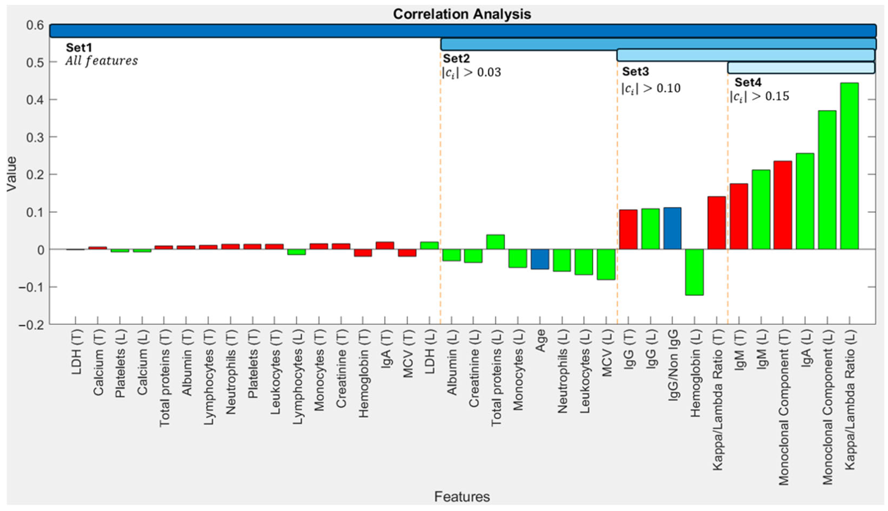
To identify input features that are most strongly associated with progression, we calculated correlation coefficients between each feature in the patient descriptors and the binary outcome (progression: 1, non-progression: 0). Coefficients approaching ±1 indicate a strong linear relationship, while values near 0 suggest a weaker relationship. Figure 4 shows these correlation coefficients, with features on the horizontal axis ordered by the absolute magnitude of their correlation with the output.

The Kappa/Lambda ratio (r = 0.444) and Monoclonal Component concentration (r = 0.371) exhibited the strongest correlations with progression (Figure 4). In general, the last recorded values (L) of indicators demonstrated stronger correlations with the outcome compared to their calculated tendencies (T) over the preceding year. Following this analysis, we performed an empirical validation to determine the most effective set of biomarkers for ML model training. For this purpose, we defined different feature sets based on correlation coefficient thresholds. Set 1 comprises all 36 features. For subsequent experiments, we only used features with an absolute correlation coefficient exceeding thresholds of 0.03 (Set 2), 0.10 (Set 3), and 0.15 (Set 4)—details in Figure 4. These criteria resulted in feature sets containing 36, 19, 11, and 6 biomarkers for Sets 1–4, respectively.

4.2.3. Overall Classifier Performance

The performance of various ML classifiers using each biomarker set is presented in

Table 3. Accuracy and F1-Score for every ML classifier trained with each set of biomarkers. Best overall results are displayed in bold. The best results of each classifier are highlighted in blue.

Classifier	Type	Set 1		Set 2		Set 3		Set 4
		Ac (%)	F1 (%)	Ac (%)	F1 (%)	Ac (%)	F1 (%)	Ac (%)	F1 (%)
DT	Fine	75.3	68.7	60.7	36.4	-	-	-	-
	Coarse	75.1	68.5	59.9	36.0	73.5	66.5	85.4	83.6
	Bagged	-	-	-	-	73.2	65.4	71.8	60.1
DA	Linear	81.1	78.0	84.2	81.8	86.3	85.1	83.7	81.0
	Subspace	82.2	79.5	84.7	82.5	90.1	89.5	90.6	89.9
LR		81.1	78.0	84.2	81.8	86.3	85.1	83.7	81.0
NB	Gaussian	49.7	47.3	76.0	69.7	75.9	71.2	82.5	80.3
	Kernel	56.4	28.3	63.2	43.1	66.2	52.9	63.4	46.0
SVM	Linear	83.3	80.8	84.5	82.0	77.6	72.5	77.8	72.2
	Coarse Gaussian	85.9	84.2	90.3	89.5	94.3	94.3	91.2	90.6
KNN	Coarse	74.2	67.7	77.3	71.2	82.0	79.3	83.0	79.9
	Weighted	60.8	39.2	65.1	47.9	-	-	-	-
	Cosine	-	-	-	-	69.1	58.3	81.6	78.3

. For conciseness, this table displays results for the two best-performing subtypes of each general classifier type. Model performance was evaluated using accuracy and F1-Score, calculated from true positives (TP), true negatives (TN), false positives (FP), and false negatives (FN) [36], according to Equations (1)–(4).

$$Accuracy\left(Ac\right)={\displaystyle \frac{TP+TN}{Total predictions}}$$

(1)

$$Precision \left(P\right)={\displaystyle \frac{TP}{TP+FP}}$$

(2)

$$Recall\left(R\right)={\displaystyle \frac{TP}{TP+FN}}$$

(3)

$$F1-Score \left(F1\right)=2{\displaystyle \frac{P\times R}{P+R}}$$

(4)

Table 3 reveals that the Coarse Gaussian SVM achieved the highest overall performance, yielding an accuracy of 94.3% with Set 3. The optimal hyperparameter configuration consisted of a kernel scale equal to 13, a constraint box C = 1, and Standardize Data = True. Subspace Discriminant Analysis also demonstrated high accuracy. Generally, ‘coarse’ variants of classifiers (e.g., Decision Tree, SVM) outperformed their ‘fine’ counterparts. Furthermore, classifiers employing non-linear decision functions (e.g., Gaussian SVM, some DA variants) tended to perform better than those restricted to linear functions.

It can be noted that one of the challenges that ML classifiers faced is that, although a data augmentation was performed, the augmented descriptors present similar features to those of the original positive patient. Consequently, there is still some imbalance in the input data, and some classifiers exhibited a tendency to classify all the patients as negative. In these cases, accuracy was not a reliable indicator of performance, which was around 50%, as approximately half of the patients were negative, but the model failed to identify positive patients. On the contrary, the F1-Score, which considers both precision and recall, provided a more representative measure. This highlighted the importance of data augmentation since no classifier would perform correctly with the original dataset due to the scarcity of positive patients.

Moreover, accuracy and F1-Score results were obtained with MLPs for every set of biomarkers. For each set of features, different configurations (e.g., number of layers, neurons per layer, and training epochs) were used during training, employing a learning rate of lr = 0.001 and the Binary Cross-Entropy loss function.

Table 4. Accuracy and F1-Score for MLPs trained with each set of features.

Set	MLP Architecture	Num. Epochs	Accuracy (%)	F1-Score (%)
1	36-16-1	10	88.0	87.7
2	19-4-1	10	90.1	89.4
3	11-4-1	5	90.9	90.9
4	6-32-16-1	3	84.2	86.2

shows the results obtained with the optimal configuration for each set.

Detailed performance metrics for the MLP models are provided in Table 4. MLPs performed competitively compared to the rest of the classifiers, surpassed consistently only by SVMs. Regarding their training, models utilizing fewer biomarkers (Sets 3 and 4) generally required fewer epochs to reach optimal performance before overfitting compared to models trained with more extensive feature sets (Sets 1 and 2). For instance, optimal results for Sets 1 and 2 were typically achieved around 10 epochs, whereas for Sets 3 and 4, approximately 3 epochs were sufficient. Although MLPs have not output the best results, which is probably due to the relatively small number of available patients, MLPs have great potential to outperform the rest of the classifiers, even SVMs, if a larger dataset is available.

4.2.4. Additional Results

In this subsection, we extracted additional data from the model predictions to enhance the explainability and transparency of these methods. First, Figure 5 displays the SHAP values obtained from the SVM model trained with Set 3, composed of the 11 most correlated features. SHAP values [37] are employed to evaluate the importance of each feature in the predictions of the model. The distance of the samples to the vertical axis of Figure 5 is proportional to the importance of that feature. Points colored pink to the right of the axis indicate that the model relates high values of the feature to progression to MM/WM. Otherwise, the model relates low values of the feature to progression.

Figure 5 shows that the SHAP values obtained from the predictions of the SVM model are consistent with the correlation analysis performed in Section 4.2.2. (see Figure 4), obtaining a similar ranking of features with both analyses. In particular, the main features considered by the model are the Monoclonal Component and the Kappa/Lambda Ratio.

Second,

Table 5. Confidence in the predictions of the SVM and MLP models.

Model	Positive (µ ± σ)	Negative (µ ± σ)	Correct (µ ± σ)	Incorrect (µ ± σ)	Total (µ ± σ)
SVM	64.0 ± 3.3	74.9 ± 9.0	70.2 ± 9.5	66.5 ± 8.5	69.7 ± 9.6
MLP	90.1 ± 7.9	86.9 ± 9.8	90.8 ± 5.3	86.5 ± 10.7	88.7 ± 10.0

includes the confidence in the prediction of the SVM and the MLP models. For the MLP, the output of the sigmoid activation function in the final layer was employed as the confidence value. Meanwhile, the SVM model provides a binary output {0,1} and a continuous score (−∞, +∞), which represents the probability that an individual belongs to a certain class. To obtain a confidence value that is equivalent to the one obtained for the MLP, the sigmoid function was employed on this confidence value to map the probability into the desired interval [0,1].

From Table 5, it can be observed that, although SVMs provided a higher accuracy, their predictions had a lower confidence than the ones obtained with the MLPs. We can also notice a different behavior of both models. If we analyze the results of SVM, it presents higher confidence in the prediction of negative patients. Meanwhile, MLPs identify positive patients with higher confidence. In general terms, correct predictions are associated with a higher confidence than incorrect predictions. This fact reinforces the reliability of these models as decision-support systems.

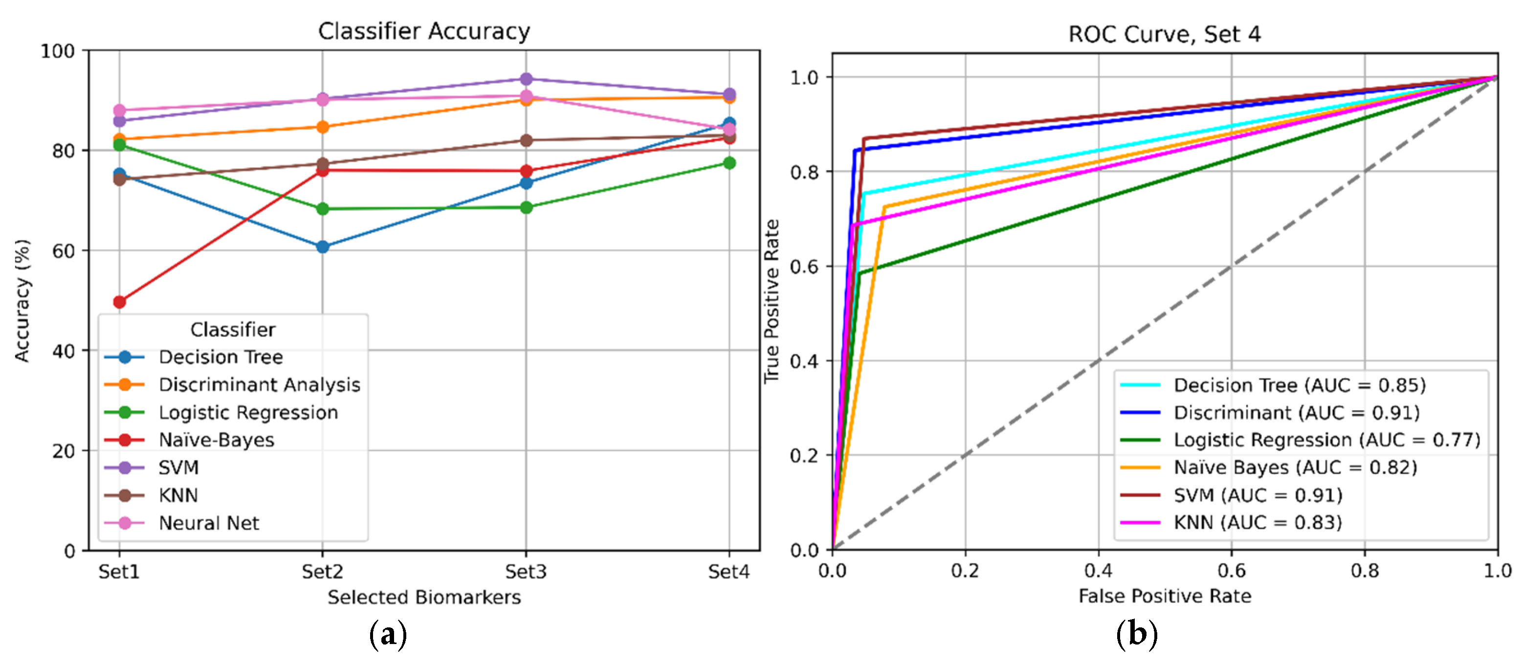
Finally, Figure 6 offers a visual comparison between the classifiers that obtained the best results overall. Figure 6a shows accuracy per experiment, and Figure 6b displays their ROC curves for Set 4.

An exhaustive comparison of results (Table 3 and Table 4, Figure 6) indicated that the best overall performance was achieved using a reduced number of highly correlated biomarkers (specifically Sets 3 and 4). This finding suggests that employing a curated selection of the most relevant biomarkers was more effective than utilizing all 36 studied indicators.

In summary, the Coarse Gaussian SVM would be the best choice for our decision support model. Also, MLPs achieved competitive performance. In particular, MLPs are tools that reach their optimal performance when large quantities of data are available. Therefore, if a larger dataset were available, this type of classifier would be expected to improve its accuracy.

5. Discussion

The findings of this study contribute to the growing body of evidence supporting the utility of machine learning in enhancing clinical decision-making, specifically in the context of MGUS. This retrospective study revealed that a Coarse Gaussian SVM achieved the highest performance among the various algorithms tested, with a 94.3% accuracy and an AUC of 0.91. These results are consistent with other studies of ML algorithms, in which SVMs and neural networks performed competitively across a variety of diagnosis tasks [25,26,27,28]. Furthermore, MLPs demonstrated promising and consistent performance.

On the one hand, SVMs showed effectiveness in high-dimensional spaces and good generalization capability, but they are computationally expensive and have limited probabilistic interpretation. On the other hand, MLPs proved to be able to learn complex and non-linear relationships, but they were prone to overfitting, and hyperparameter tuning was more complex. With access to larger datasets, MLPs may hold the potential to become highly precise and robust classifiers for this task.

A key finding was that we achieved optimal performance using a reduced set of highly correlated features (namely the monoclonal component, kappa/lambda FLC ratio, and immunoglobulin levels), with the latest recorded values of laboratory indicators exhibiting a stronger correlation to MM/WM progression compared to temporal evolutions. Importantly, no single feature emerged as a sufficiently reliable standalone predictor, underscoring the need for a multi-feature approach for effective risk stratification. A tool leveraging these key biomarkers along with an appropriate ML classifier could substantially enhance progression prediction from MGUS to MM/WM, thereby facilitating optimization of clinical resources.

Analysis of our cohort revealed that bone marrow studies were conducted in 55% classified as low risk by conventional criteria, while 27% of those deemed conventionally high-risk did not undergo BMS (data from Table 2). This observation highlights considerable variability in current clinical practice and reinforces the need for improved risk prediction models for MGUS. Consequently, the proposed model could assist clinicians in their decision-making, potentially optimizing MGUS monitoring by reducing unnecessary procedures in genuinely low-risk patients and ensuring timely, focused attention for those at higher risk.

An intrinsic challenge in MGUS risk stratification is the significant class imbalance between progressing and non-progressing patients, which is a direct reflection of the disease’s low natural progression rate. This constitutes a fundamental hurdle that any effective predictive model must overcome. For this reason, the application of data augmentation was a cornerstone of our methodology. This strategy proved crucial for robustly training and validating the machine learning classifiers, enabling them to learn the subtle patterns of progression despite the scarcity of positive cases.

It must be noted that the synthetic descriptors generated with this method are fairly similar to the original ones, which may not have completely prevented overfitting. However, employing a more pronounced noise could have compromised the performance of the model by making the generated patients too dissimilar from the original ones. Our study establishes a solid methodological foundation to validate these design choices, always with previously unseen patient data, as described in Section 4.2.1, which can be useful for future work in the field, but validating this framework on larger, multi-center cohorts with real patients is the logical next step to ensure greater generalizability.

Translating these findings into routine clinical practice requires several steps: firstly, rigorous external validation in diverse, multi-center cohorts to confirm generalizability; secondly, seamless integration into EHR systems for automated risk assessment and real-time decision support, including a user-friendly interface with actionable recommendations; and finally, comprehensive training for clinicians to effectively interpret model outputs and integrate them into workflows.

6. Conclusions

In conclusion, the machine learning-based risk stratification model developed in this study offers a promising approach to enhance the management of patients with MGUS by dynamically analyzing routinely collected laboratory biomarkers. In particular, Coarse Gaussian SVM produced the best overall results with an accuracy and F1-Score both equal to 94.3%. Although preliminary, these findings suggest that such decision-support tools could contribute to more personalized, timely, and efficient patient care pathways. Future validation with larger datasets composed solely of real patients and integration efforts will be critical to translating this potential into tangible benefits for everyday clinical practice.

Future research should explore alternative ML architectures to potentially improve predictive performance, such as Recurrent Neural Networks (RNNs), which may better capture temporal dependencies in longer sequences of laboratory data. Investigating the utility of additional biomarkers, including those derived from proteomic or genomic analyses, and other measures extracted from these biomarkers, such as the median, the volatility, or the interquartile range (IQR), could also prove valuable. Finally, continued efforts should be directed towards expanding dataset sizes through multi-institutional collaborations and broadening the spectrum of biomarkers analyzed to further refine predictive accuracy and clinical applicability.

References

- Fend, F.; Dogan, A.; Cook, J.R. Plasma cell neoplasms and related entities—Evolution in diagnosis and classification. Virchows Arch. 2023, 482, 163–177. [Google Scholar] [CrossRef] [PubMed]
- Rajkumar, S.V.; Dimopoulos, M.A.; Palumbo, A.; Blade, J.; Merlini, G.; Mateos, M.V.; Kumar, S.; Hillengass, J.; Kastritis, E.; Richardson, P.; et al. International Myeloma Working Group updated criteria for the diagnosis of multiple myeloma. Lancet Oncol. 2014, 15, 538–548. [Google Scholar] [CrossRef]
- Kyle, R.A.; Durie, B.G.; Rajkumar, S.V.; Landgren, O.; Blade, J.; Merlini, G.; Kröger, N.; Einsele, H.; Vesole, D.H.; Dimopoulos, M.; et al. Monoclonal gammopathy of undetermined significance (MGUS) and smoldering (asymptomatic) multiple myeloma: IMWG consensus perspectives risk factors for progression and guidelines for monitoring and management. Leukemia 2010, 24, 1121–1127. [Google Scholar] [CrossRef]
- Ramasamy, K.; Knight, E.; Byun, S.; Heartin, E.; Garvey, V.; Basu, S.; Stones, J.; Oakes, R.; Killingsworth, G.; Nicholls, P.; et al. Secure: A Prospective Long-Term Observational Study in Patients with Monoclonal Gammopathy of Undetermined Significance. Blood 2024, 144, 6889. [Google Scholar] [CrossRef]
- Kyle, R.A.; Larson, D.R.; Kumar, S.; Therneau, T.M.; Dispenzieri, A.; Cerhan, J.R.; Rajkumar, S.V. Long-Term Follow-up of Monoclonal Gammopathy of Undetermined Significance. N. Engl. J. Med. 2018, 378, 241–249. [Google Scholar] [CrossRef]
- Schmidt, T.; Gahvari, Z.; Callander, N.S. SOHO State of the Art Updates and Next Questions: Diagnosis and Management of Monoclonal Gammopathy of Undetermined Significance and Smoldering Multiple Myeloma. Clin. Lymphoma Myeloma Leuk. 2024, 24, 653–664. [Google Scholar] [CrossRef]
- Therneau, T.M.; Kyle, R.A.; Melton, L.J., III; Larson, D.R.; Benson, J.T.; Colby, C.L.; Dispenzieri, A.; Kumar, S.; Katzmann, J.A.; Cerhan, J.R.; et al. Incidence of monoclonal gammopathy of undetermined significance and estimation of duration before first clinical recognition. Mayo Clin. Proc. 2012, 87, 1071–1079. [Google Scholar] [CrossRef]
- Jordan, M.I.; Mitchell, T.M. Machine learning: Trends, perspectives, and prospects. Science 2015, 349, 255–260. [Google Scholar] [CrossRef] [PubMed]
- Rajkomar, A.; Dean, J.; Kohane, I. Machine learning in medicine. N. Engl. J. Med. 2019, 380, 1347–1358. [Google Scholar] [CrossRef] [PubMed]
- Beam, A.L.; Kohane, I.S. Big data and machine learning in health care. JAMA 2018, 319, 1317–1318. [Google Scholar] [CrossRef]
- Javeed, A.; Dallora, A.L.; Berglund, J.S.; Ali, A.; Ali, L.; Anderberg, P. Machine Learning for Dementia Prediction: A Systematic Review and Future Research Directions. J. Med. Syst. 2023, 47, 17. [Google Scholar] [CrossRef]
- Mohd Faizal, A.S.; Hon, W.Y.; Thevarajah, T.M.; Khor, S.M.; Chang, S.W. A biomarker discovery of acute myocardial infarction using feature selection and machine learning. Med. Biol. Eng. Comput. 2023, 61, 2527–2541. [Google Scholar] [CrossRef] [PubMed]
- Wenderott, K.; Krups, J.; Zaruchas, F.; Weigl, M. Effects of artificial intelligence implementation on efficiency in medical imaging—A systematic literature review and meta-analysis. NPJ Digit. Med. 2024, 7, 265. [Google Scholar] [CrossRef] [PubMed]
- Morita, K.; Karashima, S.; Terao, T.; Yoshida, K.; Yamashita, T.; Yoroidaka, T.; Tanabe, M.; Imi, T.; Zaimoku, Y.; Yoshida, A.; et al. 3D CNN-based Deep Learning Model-based Explanatory Prognostication in Patients with Multiple Myeloma using Whole-body MRI. J. Med. Syst. 2024, 48, 30. [Google Scholar] [CrossRef] [PubMed]
- Kasprzak, J.; Westphalen, C.B.; Frey, S.; Schmitt, Y.; Heinemann, V.; Fey, T.; Nasseh, D. Supporting the decision to perform molecular profiling for cancer patients based on routinely collected data through the use of machine learning. Clin. Exp. Med. 2024, 24, 73. [Google Scholar] [CrossRef]
- Feng, D.; Wang, Z.; Cao, S.; Xu, H.; Li, S. Identification of lipid metabolism-related gene signature in the bone marrow microenvironment of multiple myelomas through deep analysis of transcriptomic data. Clin. Exp. Med. 2024, 24, 136. [Google Scholar] [CrossRef]
- Alzubaidi, L.; Fadhel, M.A.; Al-Shamma, O.; Zhang, J.; Duan, Y. Deep Learning Models for Classification of Red Blood Cells in Microscopy Images to Aid in Sickle Cell Anemia Diagnosis. Electronics 2020, 9, 427. [Google Scholar] [CrossRef]
- Ansari, S.; Navin, A.H.; Babazadeh Sangar, A.; Vaez Gharamaleki, J.; Danishvar, S. Acute Leukemia Diagnosis Based on Images of Lymphocytes and Monocytes Using Type-II Fuzzy Deep Network. Electronics 2023, 12, 1116. [Google Scholar] [CrossRef]
- Agius, R.; Brieghel, C.; Andersen, M.A.; Pearson, A.T.; Ledergerber, B.; Cozzi-Lepri, A.; Louzoun, Y.; Andersen, C.L.; Bergstedt, J.; von Stemann, J.H.; et al. Machine learning can identify newly diagnosed patients with CLL at high risk of infection. Nat. Commun. 2020, 11, 363. [Google Scholar] [CrossRef]
- Landgren, O.; Hofmann, J.N.; McShane, C.M.; Santo, L.; Hultcrantz, M.; Korde, N.; Mailankody, S.; Kazandjian, D.; Murata, K.; Thoren, K.; et al. Association of immune marker changes with progression of monoclonal gammopathy of undetermined significance to multiple myeloma. JAMA Oncol. 2019, 5, 1293–1301. [Google Scholar] [CrossRef]
- Cowan, A.; Ferrari, F.; Freeman, S.S.; Redd, R.; El-Khoury, H.; Perry, J.; Patel, V.; Kaur, P.; Barr, H.; Lee, D.J.; et al. Personalised progression prediction in patients with monoclonal gammopathy of undetermined significance or smouldering multiple myeloma (PANGEA): A retrospective, multicohort study. Lancet Haematol. 2023, 10, e203–e212. [Google Scholar] [CrossRef]
- Cesana, C.; Klersy, C.; Barbarano, L.; Nosari, A.M.; Crugnola, M.; Pungolino, E.; Gargantini, L.; Granata, S.; Valentini, M.; Morra, E. Prognostic factors for malignant transformation in monoclonal gammopathy of undetermined significance and smoldering multiple myeloma. J. Clin. Oncol. 2002, 20, 1625–1634. [Google Scholar] [CrossRef]
- Garcea, F.; Serra, A.; Lamberti, F.; Morra, L. Data augmentation for medical imaging: A systematic literature review. Comput. Biol. Med. 2023, 152, 106391. [Google Scholar] [CrossRef]
- Claro, M.L.; de MS Veras, R.; Santana, A.M.; Vogado, L.H.S.; Junior, G.B.; de Medeiros, F.N.; Tavares, J.M.R. Assessing the impact of data augmentation and a combination of CNNs on leukemia classification. Inf. Sci. 2022, 609, 1010–1029. [Google Scholar] [CrossRef]
- Rana, M.; Bhushan, M. Machine learning and deep learning approach for medical image analysis: Diagnosis to detection. Multimed. Tools Appl. 2023, 82, 26731–26769. [Google Scholar] [CrossRef] [PubMed]
- Ghaffar Nia, N.; Kaplanoglu, E.; Nasab, A. Evaluation of artificial intelligence techniques in disease diagnosis and prediction. Discov. Artif. Intell. 2023, 3, 5. [Google Scholar] [CrossRef] [PubMed]
- Mampitiya, L.I.; Rathnayake, N.; De Silva, S. Efficient and low-cost skin cancer detection system implementation with a comparative study between traditional and CNN-based models. J. Comput. Cogn. Eng. 2023, 2, 226–235. [Google Scholar] [CrossRef]
- Dinesh, P.; Vickram, A.S.; Kalyanasundaram, P. Medical image prediction for diagnosis of breast cancer disease comparing the machine learning algorithms: SVM, KNN, logistic regression, random forest and decision tree to measure accuracy. AIP Conf. Proc. 2024, 2853, 020140. [Google Scholar] [CrossRef]
- Azar, A.T.; El-Metwally, S.M. Decision tree classifiers for automated medical diagnosis. Neural Comput. Appl. 2013, 23, 2387–2403. [Google Scholar] [CrossRef]
- Binson, V.A.; Thomas, S.; Subramoniam, M.; Arun, J.; Naveen, S.; Madhu, S. A Review of Machine Learning Algorithms for Biomedical Applications. Ann. Biomed. Eng. 2024, 52, 1159–1183. [Google Scholar] [CrossRef]
- Bohra, H.; Arora, A.; Gaikwad, P.; Bhand, R.; Patil, M.R. Health prediction and medical diagnosis using Naive Bayes. Int. J. Adv. Res. Comput. Commun. Eng. 2017, 6, 32–35. [Google Scholar] [CrossRef]
- Sievering, A.W.; Wohlmuth, P.; Geßler, N.; Gunawardene, M.A.; Herrlinger, K.; Bein, B.; Arnold, D.; Bergmann, M.; Nowak, L.; Gloeckner, C.; et al. Comparison of machine learning methods with logistic regression analysis in creating predictive models for risk of critical in-hospital events in COVID-19 patients on hospital admission. BMC Med. Inform. Decis. Mak. 2022, 22, 309. [Google Scholar] [CrossRef]
- Rojas-Domínguez, A.; Padierna, L.C.; Valadez, J.M.C.; Puga-Soberanes, H.J.; Fraire, H.J. Optimal hyper-parameter tuning of SVM classifiers with application to medical diagnosis. IEEE Access 2017, 6, 7164–7176. [Google Scholar] [CrossRef]
- Beretta, L.; Santaniello, A. Nearest neighbor imputation algorithms: A critical evaluation. BMC Med. Inform. Decis. Mak. 2016, 16, 197–208. [Google Scholar] [CrossRef] [PubMed]
- Cui, Y.; Hong, X.; Yang, H.; Ge, Z.; Jiang, J. AsymUNet: An Efficient Multi-Layer Perceptron Model Based on Asymmetric U-Net for Medical Image Noise Removal. Electronics 2024, 13, 3191. [Google Scholar] [CrossRef]
- Juba, B.; Le, H.S. Precision-recall versus accuracy and the role of large data sets. In Proceedings of the AAAI Conference on Artificial Intelligence, Honolulu, HI, USA, 27 January–1 February 2019; Volume 33, pp. 4039–4048. [Google Scholar]
- Liu, Y.; Liu, Z.; Luo, X.; Zhao, H. Diagnosis of Parkinson’s disease based on SHAP value feature selection. Biocybern. Biomed. Eng. 2022, 42, 856–869. [Google Scholar] [CrossRef]