Out-of-Stock Predicting Out-of-Stock Risk Under Delivery Schedules Using Neural Networks

Abstract

In retail logistics, one typical task is to arrange a delivery schedule that guides the intake of inventory from the distribution center to stores. It is essential to accurately predict the out-of-stock (OOS) outcome for various delivery schedules to identify the optimal patterns for minimizing the OOS ratio. This paper investigates the feasibility of utilizing a neural network to accurately predict the out-of-stock (OOS) risk under each delivery pattern. Due to the zero-inflated distribution of the target values, it is necessary to evaluate two prediction accuracies simultaneously: the accuracy on data with a positive ground truth OOS rate and the accuracy on data with a zero ground truth OOS rate. In this paper, I examine how a selection of features associated with delivery schedules and the choice of activation function at the output layer, would impact the accuracy of the model.

1. Introduction

In retail operations, the supply chain is crucial for balancing supply with consumer demand effectively. For the retail business, it involves multiple typical stages. Products are manufactured in a factory and are then transported to the distribution center (warehouse). Individual retail stores, based on the current sales status and future sales expectations, place a purchasing order to the warehouse, and the items are delivered to the stores. The delivery from the warehouse to the store, which is closest to the store’s operational side, directly impacts the store’s inventory status.

One important performance index for the supply chain in the retail business is the out-of-stock (OOS) probability, i.e., the probability of an event where the inventory level reaches zero and customers are unable to purchase the product. It is well-known that products being OOS can lead to customer dissatisfaction, lost sales, and a tarnished brand reputation. It reduces the potential impact of promotions and distorts actual demand. It impacts brand loyalty, promotes competitors’ brands, and diminishes the efficiency of the sales team [1,2,3,4]. Over the past several decades, OOS events have been a central topic of research and are a critical area of study within retail operations [2,5].

Despite considerable efforts to mitigate the frequency of OOS events, they remain prevalent and lead to substantial losses within the retail industry. According to [6], it is estimated that OOS events account for approximately 4% of total annual revenue globally in the retail sector, resulting in a staggering USD 984 billion in losses.

To control the OOS risk, a reasonable delivery schedule that specifies when to order and when each order will arrive is essential. A schedule for delivery from the warehouse to the store specifies clearly the days on which orders are placed and determines the appropriate lead times. In many real-world retail and supply chain settings, delivery schedules are not continuously adjustable but instead follow fixed weekly or cyclical patterns, i.e., once set, altering such schedules can be challenging due to adjustment costs, which encompass expenses related to supply chain realignment, supplier negotiations, and logistical coordination. Retailers often operate under structured weekly ordering and delivery cadences to align procurement, distribution, and replenishment across multiple locations. As supported by both industry practices and the academic research, weekly delivery cycles are a common and realistic feature in supply chain operations [7,8,9].

To determine the optimal delivery schedule from a business perspective, it is crucial to assess the impact of various order schedules on inventory performance, which requires understanding their effect on the OOS ratio. In a typical logistics scenario, the delivery schedule repeats regularly, typically on a weekly or monthly basis. Usually, the primary interest is in understanding the average OOS ratio for each day of the week, from Monday to Sunday, under each delivery schedule.

One straightforward way to assess the impact is to use simulation, i.e., for each store and each product, using historical data to simulate inventory dynamics under various delivery schedules, and to analyze the resulting OOS rates. While simulation offers insights into these outcomes, it often resource-intensive. Often, retail stores use batched delivery, i.e., aggregating multiple orders for delivery in a single trip, which improves efficiency and potentially reduces costs for retailers. To fully understand the impact of the delivery schedule on the store’s out-of-stock ratio, it is necessary to simulate the daily inventory evolution for each product. If a store has a large number of products, the computation will be demanding and the computation time long. To alleviate such a computational burden, it is necessary to develop predictive models that utilize order schedule data to forecast the OOS rates, providing valuable decision support.

The task of this paper is to develop a model that, using the delivery schedule as input, can predict the average out-of-stock (OOS) ratio for each day of the week. However, this task presents a significant challenge: the OOS ratio is a number between 0 and 1, and, in reality, OOS events occur with a small probability. This means that the target variable has zero-inflated values. In such a case, a single accuracy metric is insufficient to reflect the accuracy of the model. This paper focuses on the following two metrics:

• Mean absolute error on zero-OOS data ($MA{E}_0$): This metric measures the average absolute error between the predicted OOS rate and zero for instances where the ground truth OOS rate is zero. It quantifies the model’s false alarms, with higher values indicating that the model is predicting too many OOS events when there are none.
• Average percentage error on positive-OOS data ($MAP{E}_{+}$): This metric calculates the average of the absolute percentage error between the predicted and actual OOS rates, specifically for instances where the ground truth OOS rate is positive. This metric assesses the model’s ability to detect OOS events accurately.

Our main research question is the following: What modeling strategy can be used to raise the accuracy of prediction, i.e., improve both metrics? To be more specific, I study the two following research questions:

Q1: What delivery schedule feature combination can reach the best performance on both metrics?

Several key features must be considered, including the day of the order decision, lead time, and arrival date. Logically, knowing any two of these features can often determine the third. However, from a deep learning perspective, it is unclear whether it is sufficient to include only a subset of these features or if all of them must be included. Moreover, do these features contribute equally to the model’s prediction accuracy? Answering these questions will help clarify how delivery schedule information impacts OOS predictions, providing valuable insights for other machine learning tasks that involve delivery schedules and OOS rates as target variables. To address this, I explore different combinations of these features and compare their performance.

Q2: What activation function of the output layer can achieve better performance on both metrics, ReLU or Sigmoid?

Given that the OOS rate is a non-negative value bounded between 0 and 1, two common choices for the output layer activation function are ReLU and Sigmoid. How do these activation functions affect model performance in terms of both metrics, and what are the underlying reasons for these effects? Despite the widespread use of both activation functions, the previous literature has not fully explored their comparative impact in the context of OOS rate prediction. Understanding this will provide valuable insights into how different model architectures influence prediction accuracy.

The contributions of this paper are multi-faceted: First, this is one of the few studies that formally addresses the prediction of OOS rates under different delivery schedule configurations using a deep learning framework, providing practical guidance for industrial use cases. Second, it is among the few studies that compare ReLU and Sigmoid activation functions in the context of non-negative bounded target variables.

The paper is organized as follows: Section 2 provides a literature review. Section 3 presents the problem setup and illustrates some key concepts related to the research questions. Section 4 presents experiments using simulated sales data, including the experiment setup and results. Section 5 presents the results of experiments using real-world retail sales data. Section 6 concludes the paper.

2. Literature Review

This paper is closely related to the optimization of cyclical or fixed-schedule ordering policies. For example, ref. [7] examined cyclic delivery strategies in one-warehouse, multi-retailer systems, demonstrating their near-optimality under dynamic demand. Similarly, ref. [9] formulated a joint cyclic production and delivery scheduling model for two-stage supply chains, capturing the coordination between upstream and downstream operations. Ref. [8] provided empirical evidence that scheduled ordering often outperforms unstructured policies in distribution supply chains. While these studies emphasize the cost-efficiency and operational stability of cyclical delivery planning, few have incorporated such constraints into data-driven OOS risk prediction models. Our work contributes to this intersection by explicitly modeling out-of-stock risks under fixed delivery schedules, thereby bridging a methodological gap between predictive modeling and scheduling-aware logistics planning.

This paper is also closely related to the prediction of out-of-stock (OOS) events in inventory management [10,11]. One major area of focus has been on identifying the drivers of OOS events. For instance, ref. [12] conducted a systematic review of the factors influencing retail on-shelf availability. These drivers can be broadly categorized into two groups: retail store practices and upstream challenges within the retail supply chain. Examples of the first category include inventory inaccuracies, shrinkage, and inefficient shelf replenishment processes. The second category pertains to issues relating to forecasting inaccuracies. For example, ref. [13] proposed that one factor contributing to stock-out issues is the presence of fast-selling items, suggesting that implementing echelon inventory policies could help reduce short-term forecast errors. Additionally, ref. [14] proposed a hybrid artificial neural network for developing a sales forecasting model specifically for fresh food. This paper differs from these aforementioned papers in that, instead of focusing on sales prediction, the accuracy of which is a reason for OOS events, this paper directly addresses the prediction of OOS risks.

This paper is also related to the study of experimental model architectures. For example, ref. [15] critically analyzed and studied the comparative performance of two ReLU and Sigmoid activation-based models. Ref. [16] reviewed and compared the commonly used activation functions for deep neural networks. Ref. [17] compared the performance of the rectified linear unit (ReLU) and Sigmoid activation functions on CNN models for animal classification. Ref. [18], by applying concepts from the statistical physics of learning, studied layered neural networks of rectified linear units (ReLUs), and compared them with Sigmoidal activation functions. This paper differs from the previous literature in that, while the latter primarily considers the activation function in hidden layers, this paper focuses mainly on the activation function at the output layer.

3. Problem Setup: Typical Delivery Scheduling

Suppose a retail store is determining its weekly delivery schedule, i.e., which days of the week it will issue order instructions to the warehouse and how many days it will take for the ordered inventory to arrive, i.e., the lead times. The schedule, once determined, cannot be changed for an extended period. For simplicity, we only consider the ordering schedule for a single product.

We define the following quantities:

• $D_t$: Actual sales at day t.
• ${\widehat{D}}_t$: Sales forecast for day t.
• $S_t$: Actual store inventory quantity at the end of day t.
• ${\widehat{S}}_t$: Forecasted store inventory quantity at the end of day t.
• $I_t$: Intake quantity at day t (i.e., arrival of orders).
• $I_t$: Order quantity.

For each day of the week when an order will be placed, assuming that the lead time is l, the store needs to calculate the following items:

• Forecasted Inventory (${\widehat{S}}_{t+l},0)$: The forecasted inventory is computed as the difference between the current inventory at the end of the day and the forecasted sales during the lead time, adjusted for any intake from previous orders.
• Future Forecasted Sales (${\widehat{D}}_{t+l+1:t+1+l^{\prime }}$): This is the sum-up of the forecasted sales data between the arrival of this order and the arrival of the next order (supposing that the lead time of the next order day is $l^{\prime }$).

Once the forecasted inventory is calculated, the order quantity is determined as the difference between the future forecasted sales for the next period and the forecasted inventory at the time of the order:

$$Q_t=max({\widehat{D}}_{t+l+1:t+1+l^{\prime }}-{\widehat{S}}_{t+l},0)$$

(1)

where

$${\widehat{S}}_{t+l}=max(S_t-{\widehat{D}}_{t,t+l},0)$$

(2)

In other words, on each day of the week when the store places an order, the ordering quantity is calculated such that the store has enough inventory to meet future demand until the next order arrives. Also, no order is placed if the forecasted inventory is sufficient (i.e., if the difference is negative or zero).

The order quantity at day t is the intake quantity of day $t+l$:

$$I_{t+l}=Q_t$$

(3)

Through this process, the store’s actual inventory evolves daily as

$$S_t=max(S_{t-1}+I_t-D_t,0)$$

(4)

In other words, the inventory at the end of the current day is the inventory level at the end of one day plus the intake of the current day minus the current day’s sales. An OOS event happens whenever $S_{t-1}+I_t-D_t<0$ occurs.

This paper focuses on the average out-of-stock rate for each day of the week, specifically, the average OOS rate for Monday, Tuesday, and so on. It is evident that the more frequently the order is placed, the lower the overall OOS rate. The purpose of this paper is to understand the OOS rate under each delivery arrangement quantitatively.

It is usually challenging to simulate outcomes for all order patterns due to time and computer resource constraints. For example, if I consider that the lead time can be as long as 5 days and stores can order as many as six times a week, there would be 3630 different possible order schedule patterns. Moreover, there may be multiple stores, and simulating all patterns for each store individually can be computationally demanding. Therefore, it is essential to consider using a model to predict the OOS rate for each day of the week.

In the context of this study, various inputs are explored to determine the optimal order schedule and its impact on the out-of-stock ratio in retail logistics. Each input plays a significant role in capturing specific aspects of the ordering and inventory management process.

The first input is the day of the week on which the order is executed. This vector specifies the days on which a store places orders for restocking inventory. The order day of the week is represented as a vector in the model, where each element corresponds to one of the seven days (Monday to Sunday). This enables the model to identify the pattern and frequency of orders for each specific day.

The second input is the lead time vector, which is the number of days between placing an order and receiving the goods. It is a critical factor in inventory management as it influences when a store can expect to restock its inventory. The model uses a vector to represent the lead time for each day of the week. This vector represents the number of days it takes for orders placed on each day to be delivered. The lead time is also described as a one-hot encoded vector.

The third input to consider is the vector representing the days of the week when intake occurs, i.e., the day on which orders arrive at the store, based on the lead time from the order date. For example, if the store places an order on Monday with a 2-day lead time, the arrival day will be Wednesday. The arrival day is also represented as a one-hot encoded vector similar to the order day. This input is essential because it helps the model understand the timing of when the inventory is restocked, which directly impacts the availability of stock and the likelihood of running out of stock.

Finally, we have the day of the week, which represents the specific day for which the out-of-stock prediction is being made. Each sample in the dataset corresponds to a particular day, and this input helps the model understand which day’s out-of-stock behavior is being evaluated. The day of the week is also one-hot encoded to match the format used for the other time-based inputs.

I next provide an example of how a specific delivery schedule is transformed into the above features. Consider a schedule where the store performs the following actions:

• Places an order on Monday, which arrives on Thursday (lead time: 3 days).
• Places an order on Wednesday, which arrives on Sunday (lead time: 3 days).
• Places an order on Thursday, which arrives on the next Monday (lead time: 4 days).

Consider a data point on Thursday. The feature inputs are as follows:

• Order days of week: $[1,0,1,1,1,0,0]$;
• Lead time: $[3,0,3,3,4,0,0]$;
• Arrival days of week: $[1,0,0,1,0,1,1]$.

Each of these inputs is designed to capture a distinct aspect of the ordering and inventory replenishment process. It is clear that each of the features above serves a purpose, and all of them should be included in the model to achieve the best accuracy. What is not straightforward, however, is the role of these features in improving the two metrics mentioned in the previous sections. Are some of them critical for model performance? And can some of them be excluded, given that the critical ones have been added? To explore these questions, an experiment is needed that compares the performance of models with different feature inputs.

4. Numerical Experiment

In this section, to perform the analysis, I simulate a demand data series, perform an inventory simulation under each delivery schedule using the demand data, and compute the average OOS probability of each day of the week. I then use the laboratory data to train neural network models and study the three research questions.

4.1. Data

This section explains the process of generating actual sales and forecasted sales data and simulating the inventory dynamics based on sales under each delivery schedule.

To simulate realistic daily demand patterns, I adopt a stochastic process with both temporal dependence and calendar-based seasonality. Specifically, I generate daily sales $D_t$ using an ARMA(2,2) process defined as follows:

$$D_t^{*}={\varphi }_1{D}_{t-1}^{*}+{\varphi }_2{D}_{t-2}^{*}+{\epsilon }_t+{\theta }_1{\epsilon }_{t-1}+{\theta }_2{\epsilon }_{t-2},$$

(5)

where $\left\{{\epsilon }_t\right\}$ is a white noise process. In our implementation, the parameters are set to ${\varphi }_1=0.5$, ${\varphi }_2=-0.25$, ${\theta }_1=0.4$, and ${\theta }_2=-0.3$. The raw series $D_t^{*}$ is then shifted and scaled to ensure non-negativity and calibrated to a base sales level of approximately 100 units:

$$D_t=\mathrm{round}\left(100+10·(D_t^{*}-\underset{t}{min}{D}_t^{*})\right).$$

(6)

To incorporate weekly seasonality, I increase sales by 30% on weekends:

$$D_t\leftarrow \mathrm{round}(1.3·D_t),\mathrm{if}t\in \left\{\mathrm{Saturday},\mathrm{Sunday}\right\}.$$

(7)

I apply a simple averaging method to create forecasted sales data. For each week, I predict the sales of each day using the average of L weeks of data:

$${\widehat{D}}_t=\sum _{l=1}^{l=L}{D}_{t-l\ast 7}$$

(8)

Using the actual sales series and forecasted series, along with the order quantity determination from the previous sections, I can simulate the order quantity and resulting inventory dynamics under each delivery schedule.

I restrict the delivery schedule to meet the following conditions:

• The possible lead time ranges from 1 day to 5 days.
• If batch 1 is earlier than batch 2, the arrival day of batch 1 should also be earlier than that of batch 2.

The following graph illustrates an example of the daily inventory evolution under a specific delivery schedule for a specific store. As shown in Figure 1, the inventory (green line) occasionally drops to zero, resulting in an out-of-stock situation.

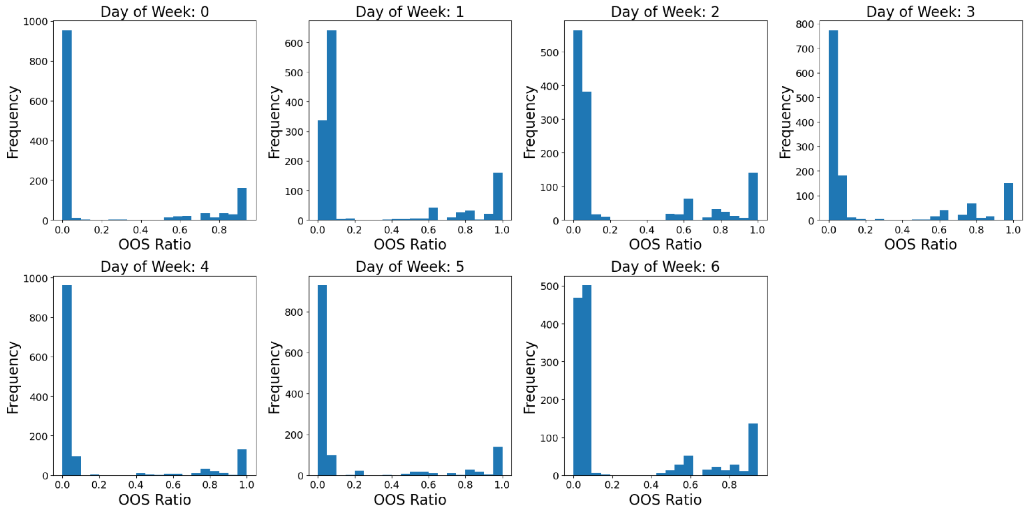
The data for training are created such that, for each delivery pattern and day of the week, I compute the ratio of days where the end-of-day inventory is zero, i.e., an OOS event happens.

Figure 2 shows the resulting distribution of the average OOS rate for each day of the week. It contains the results of 1500 randomly picked delivery schedules, each being applied to the same simulated demand series data. The distribution indicates that a considerable portion of the OOS rate is zero, and only a small part of the data has a positive OOS rate.

Table 1. Configuration settings used for model training.

Parameter	Value
Optimizer	Adam
Learning rate	0.001
Loss function	Mean Squared Error (MSE)
Activation function	ReLU or Sigmoid (varied across experiments)
Hidden layers	3 (dense layers: 128, 64, 32 units)
Output layer activation	ReLU or Sigmoid
Epochs (max)	30
Batch size	32
Early stopping patience	20

summarizes the configuration of the model training.

4.2. Model and Training

Figure 3 illustrates the neural network structure used for training the model. Taking delivery schedule-related features as input, the information goes through three dense layers, with the number of neurons being 128, 64, and 32, respectively. In the output layer, I consider two activation function options: ReLU and Sigmoid.

The input is the delivery schedule and the day of the week, and the target variable is the average OOS rate on that day of the week. I use the metrics mentioned in the introduction section to evaluate the model. Specifically, for each model, I compute the mean absolute percentage error (MAPE) for data with a positive out-of-sample (OOS) rate and the mean absolute error (MAE) for zero-OOS-rate data for each day of the week on the test data. I then take the simple average over 7 days for these two metrics. As a result, each model has two values to indicate its performance on test data.

The model architecture follows a common design principle where the number of neurons is gradually reduced in successive dense layers (128 → 64 → 32). This “funnel” structure is widely adopted in neural networks as it encourages hierarchical feature abstraction—the earlier layers capture a wide variety of low-level patterns from the input features, while the later layers progressively condense this information into more abstract and task-specific representations. This reduction in dimensionality also helps mitigate overfitting by forcing the network to compress and generalize the input representations rather than memorize them. The specific layer sizes (128, 64, 32) are chosen empirically based on performance on the validation set and represent a trade-off between model expressiveness and training stability.

In this simulation study, for each run, I randomly pick a proportion of delivery patterns. For each of the delivery patterns, for each store, I simulate the inventory dynamics and calculate the average out-of-stock ratio for each day of the week. The dataset is then split using a random-shuffle strategy, with 80% of the samples used for training and 20% for testing. For each run, each model faces the same data and the same data split. The uncertainty of model performance thus comes from the random sampling of stores and delivery patterns, and the random split of the dataset.

4.3. Feature Combination and Model Performance

This section studies the model performance under various feature combinations.

I consider the following feature combinations:

• Model 0: order days of week, lead times, and day of week;
• Model 1: lead times, arrival days of week, and day of week;
• Model 2: order days of week, arrival days of week, and day of week;
• Model 3: order days of week, lead times, arrival days of week, and day of week;
• Model 4: arrival days of week and day of week;
• Model 5: lead times and day of week.

To explore the contribution of different delivery schedule-related features, I design six models (Model 0 to Model 5), each representing a specific combination of order days, lead times, arrival days, and day of the week. These combinations are not chosen exhaustively but are designed based on domain knowledge and empirical intuition: the lead time vector is hypothesized to carry the richest information, as it implicitly encodes both ordering and arrival logic. Some combinations (e.g., Models 2 and 4) are included to test whether the model can learn lead time information indirectly from the order and arrival days. Other combinations (e.g., Models 1 and 3) are used to examine the incremental value of adding redundant or complementary features. Although I do not employ an automated feature selection strategy, such as greedy or forward selection, this structured comparison enables us to assess the marginal utility of individual features and their interactions in a controlled manner.

Table 2. Model performance summary (Sigmoid activation in output layer).

Model	MAPE+	MAE0	Ranks (MAPE+/MAE0)
3	0.100 (0.013)	0.020 (0.007)	1/1
1	0.102 (0.014)	0.021 (0.008)	2/2
0	0.154 (0.019)	0.038 (0.012)	3/3
5	0.183 (0.017)	0.048 (0.009)	4/4
2	0.226 (0.026)	0.074 (0.014)	5/5
4	0.356 (0.025)	0.136 (0.025)	6/6

and

Table 3. Model performance summary under ReLU activation (mean (SD)).

Model	MAPE+	MAE0
0	0.173 (0.016)	0.029 (0.009)
1	0.120 (0.014)	0.013 (0.009)
2	0.248 (0.019)	0.060 (0.014)
3	0.111 (0.011)	0.016 (0.007)
4	0.355 (0.020)	0.118 (0.014)
5	0.207 (0.019)	0.033 (0.010)

reveal the ranking for model performance under Sigmoid and ReLU activation in the output layer. The results are the same for both metrics:

• Best tier: Models 3 and 1. They are significantly better than the other models, but they are statistically indistinguishable from each other.
• Middle tier: Model 0. It is significantly worse than the top tier, but better than Models 5, 2, and 4.
• Lower tier: Model 5, then Model 2, with Model 4 being clearly the worst for both metrics.

Table 4. Pairwise statistical tests between models (Sigmoid activation in output layer): p-values from paired t-tests and Wilcoxon signed-rank tests.

Model A	Model B	MAPE+ t-Test	MAPE+ Wilcoxon	MAE0 t-Test	MAE0 Wilcoxon
0	1	0.0000	0.0000	0.0000	0.0000
0	2	0.0000	0.0000	0.0000	0.0000
0	3	0.0000	0.0000	0.0000	0.0000
0	4	0.0000	0.0000	0.0000	0.0000
0	5	0.0000	0.0000	0.0019	0.0032
1	2	0.0000	0.0000	0.0000	0.0000
1	3	0.4720	0.3535	0.4080	0.4060
1	4	0.0000	0.0000	0.0000	0.0000
1	5	0.0000	0.0000	0.0000	0.0000
2	3	0.0000	0.0000	0.0000	0.0000
2	4	0.0000	0.0000	0.0000	0.0000
2	5	0.0000	0.0001	0.0000	0.0000
3	4	0.0000	0.0000	0.0000	0.0000
3	5	0.0000	0.0000	0.0000	0.0000
4	5	0.0000	0.0000	0.0000	0.0000

and

Table 5. Pairwise statistical tests between models (ReLU activation): p-values from paired t-tests and Wilcoxon signed-rank tests.

Model A	Model B	MAPE+ t-Test	MAPE+ Wilcoxon	MAE0 t-Test	MAE0 Wilcoxon
0.0	1.0	0.0000	0.0000	0.0000	0.0000
0.0	2.0	0.0000	0.0000	0.0000	0.0000
0.0	3.0	0.0000	0.0000	0.0000	0.0000
0.0	4.0	0.0000	0.0000	0.0000	0.0000
0.0	5.0	0.0000	0.0000	0.0057	0.0105
1.0	2.0	0.0000	0.0000	0.0000	0.0000
1.0	3.0	0.0061	0.0115	0.2955	0.2897
1.0	4.0	0.0000	0.0000	0.0000	0.0000
1.0	5.0	0.0000	0.0000	0.0000	0.0000
2.0	3.0	0.0000	0.0000	0.0000	0.0000
2.0	4.0	0.0000	0.0000	0.0000	0.0000
2.0	5.0	0.0000	0.0000	0.0000	0.0000
3.0	4.0	0.0000	0.0000	0.0000	0.0000
3.0	5.0	0.0000	0.0000	0.0000	0.0000
4.0	5.0	0.0000	0.0000	0.0000	0.0000

, through pairwise statistical tests, further support the ranking of the above models.

The results indicate that the lead time vector is critical for model accuracy. Models 4 and 2, which lack lead time information, perform the worst, while Model 5, which includes lead time alone, achieves moderate performance. One possible reason behind this is that the lead time vector itself already embeds all the information of the delivery schedule: the non-zero elements indicate orders to be placed, and the numbers represent the corresponding lead times. The arrival days of information can be derived from them. Furthermore, a comparison of Models 2 and 4 shows that the neural network is unable to infer lead time information from the order days of the week and arrival days of the week.

The results of Models 0, 1, and 3 indicate that, conditioning on the existence of lead time vectors, the arrival days of the week are more effective than the order days of the week in predicting the OOS rate. To be specific, Model 0, which has an order day of the week and lead time vector, performs worse than Model 1, which has the arrival day of the week and lead time vectors. Moreover, Models 1 and 3 have nearly identical model performance, indicating that, when the arrival day of the week is included, adding the order day of the week does not improve the model. On the other hand, Models 0 and 3 indicate that, when the order day of the week is present, adding the arrival day of the week still improves model accuracy. The possible reason behind this is that the arrival days of the week directly indicate the day of the week when there is intake, and usually the OOS rate is low on these days. As a result, this arrival day of the week is directly associated with the OOS results.

4.4. Impact of Activation Function

This section studies the model performance under different activation functions (ReLU and Sigmoid) in the output layer.

First, we examine the performance using the feature input of Model 3. Only Model 3 is chosen for the activation function analysis because it exhibits the best overall performance across both MAPE₊ and MAE₀ metrics (see Section 4.2). It also incorporates all feature groups—order day, lead time, arrival day, and day of the week—thus representing the most comprehensive and expressive model configuration among Models 0–5. I also evaluate the performance of ReLU and Sigmoid across the other models. The results confirm a consistent pattern, and I evaluate two common activation functions at the output layer: ReLU (rectified linear unit) and Sigmoid. The ReLU function is defined as follows:

$$ReLU\left(x\right)=max(0,x)$$

(9)

It outputs zero for negative inputs and passes positive values unchanged, producing sparse and non-negative outputs.

The Sigmoid function is defined as follows:

$$\sigma \left(x\right)={\displaystyle \frac{1}{1+e^{-x}}}$$

(10)

It maps any real-valued input to a value strictly between 0 and 1, making it particularly suitable for bounded output variables like the out-of-stock (OOS) rate.

Table 6. Activation comparison on Model 3 (mean (SD)).

Activation	MAPE+	MAE0	Overprediction Ratio+
ReLU	0.118 (0.016)	0.0157 (0.0086)	0.354 (0.087)
Sigmoid	0.099 (0.009)	0.0222 (0.0128)	0.280 (0.066) *

* Difference vs. ReLU is statistically significant at $p<0.05$ (paired t-test and Wilcoxon signed-rank test). The paired t-test on the overprediction ratio shows Sigmoid significantly outperforms ReLU ($t_{14}=-2.67$, $p=0.016$; Wilcoxon $p=0.027$).

presents the results of the model using ReLU and the model using Sigmoid. Overall, the results suggest that models with Sigmoid activation tend to achieve a lower average WAPE on positive OOS data but exhibit a higher mean absolute error on zero OOS data compared to those with ReLU.

There are two possible factors contributing to the model’s better performance with the Sigmoid function on positive data compared to the model with the ReLU function. One obvious factor is that the Sigmoid activation function ensures that the output is between 0 and 1, which is the range of the OOS rate. On the other hand, for ReLU, the output is unbounded upward, meaning it can exceed 1.

Another contributing factor, which is more nuanced, is the difference in prediction tendencies: ReLU tends to underpredict, while Sigmoid tends to overpredict. This pattern is further illustrated in Table 6, which compares the two activation functions in terms of the WAPE and overprediction ratio for positive OOS data. The overprediction ratio is defined as the proportion of cases where the predicted OOS value exceeds the actual value. The figure shows that, for most pairs, the model with ReLU activation exhibits a lower overprediction ratio than its Sigmoid counterpart.

This discrepancy may stem from differences in the gradients used for parameter updates during training. When the output layer uses ReLU activation, the derivative is 1 for positive outputs, meaning the gradient of the loss function scales directly with the difference between the actual and predicted values. Consequently, large actual values lead to larger gradients and, therefore, larger parameter updates. In contrast, the derivative of the Sigmoid function varies: it increases for negative inputs (i.e., outputs below 0.5) and decreases for positive inputs (i.e., outputs above 0.5), reaching its maximum at an output of 0.5. Thus, for large target values, the activation derivative may be small, leading to smaller gradients and less responsive parameter updates. As a result, models with Sigmoid activation are less sensitive to large target values compared to those using ReLU, leading to a lower overprediction ratio than the model with ReLU.

The reason for the worse performance of the Sigmoid function in terms of the MAE with zero OOS data is that the Sigmoid function is not exactly zero even when the input is extremely large; the function value is close to zero, but still larger than zero. Therefore, with zero OOS data, a model using a Sigmoid function will tend to yield many small positive predictions. On the other hand, the ReLU function returns a value of exactly zero when the input is negative. As a result, the model with Sigmoid activation will have a (slightly) worse performance on zero OOS data than the model with the ReLU activation function.

5. Case Study

The previous section examined the impact of delivery schedule-related features and the activation function at the output layer. To verify whether the conclusions can be applied to real-world sales data, this section re-conducts the experiments using a real-world retail sales dataset as a case study.

I use a dataset from Kaggle, a data science competition platform and online community for data scientists and machine learning practitioners. It is derived from a competition to predict store sales at Rossmann, which operates over 3000 drugstores in seven European countries. The dataset comprises the daily sales of each location over more than two years. Although the sales data in this dataset are aggregated across various drug products, for simplicity, I regard each store as selling only a single drug product. (Originally, the task of this competition was to predict 6 weeks of daily sales for 1115 stores located across Germany. The purpose of this paper is not to make predictions. I simply use the dataset to obtain an approximation of real-world retail sales data. The link to the Kaggle page is https://www.kaggle.com/competitions/rossmann-store-sales/overview. 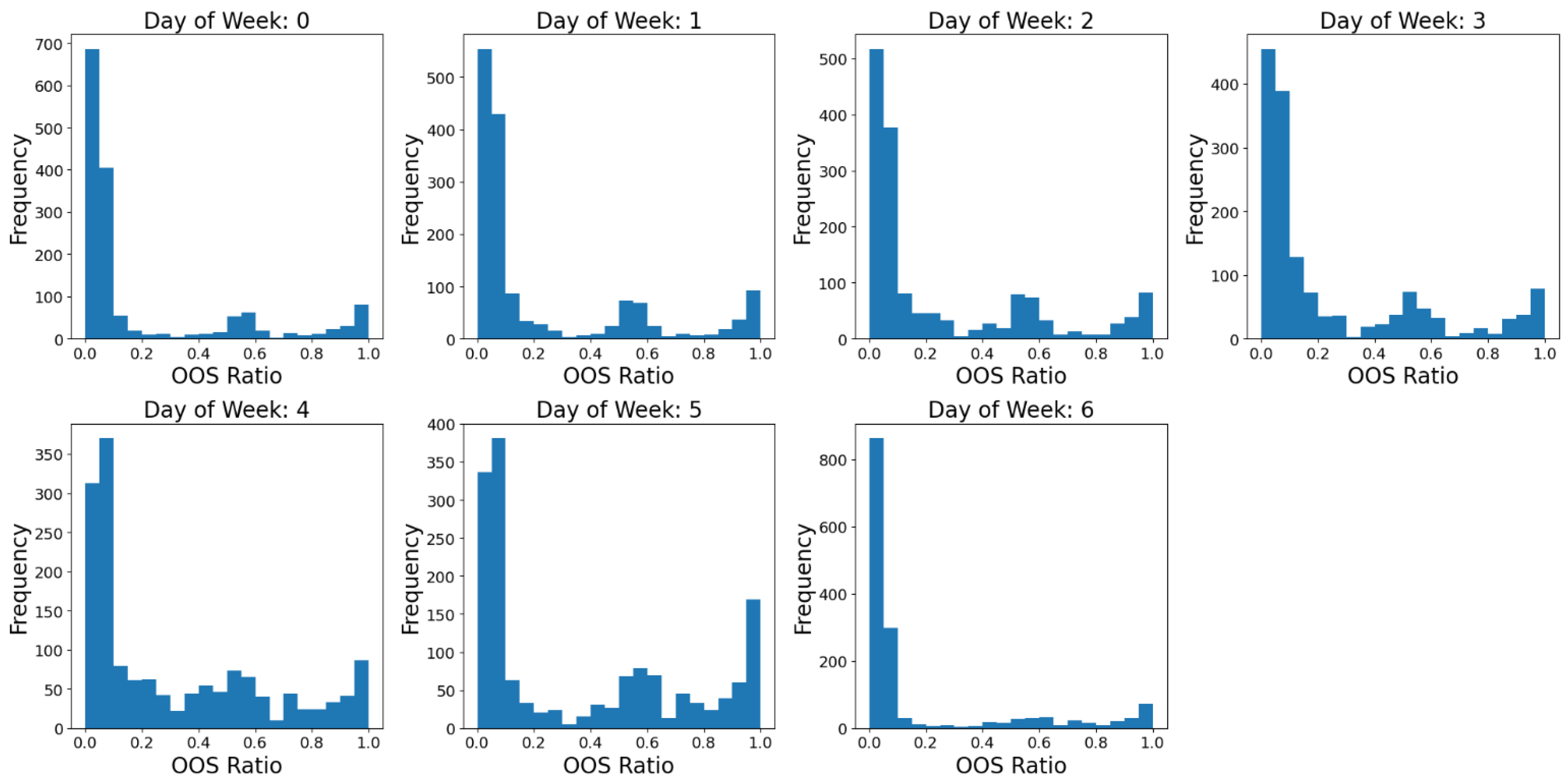accessed on 12 June 2025) Figure 4 shows that, with this realistic sales data, the OOS distribution of each day of the week is still zero-inflated.

In this case study, for each run, I randomly pick some stores and pick a proportion of delivery patterns. For each of the delivery patterns, at each store, I simulate the inventory dynamics and calculate the average out-of-stock ratio for each day of the week. The dataset is then split using a random-shuffle strategy, with 80% of the samples used for training and 20% for testing. For each run, each model faces the same data and the same data split. The uncertainty in model performance thus stems from the random sampling of stores and delivery patterns, as well as the random split of the dataset.

5.1. Experiment on Input Feature

In this case study, I compare the forecasting performance of five models (Model 0 to Model 4) across multiple experimental runs in terms of the MAPE₊ and MAE₀. One difference from the previous experiment using simulated data set is that, here, a feature that indicates the store type is added an additional feature for all models. This feature is a categorical variable, so in the model training it is first turned to one-hot encoded vector before inputting into the model.

Table 7. Model performance summary (Sigmoid-based models).

Model	MAPE+	MAE0	Ranks (MAPE+/MAE0)
3	0.095 (0.005)	0.0218 (0.0044)	1/1
1	0.095 (0.005)	0.0240 (0.0039)	2/2
0	0.113 (0.0067)	0.0359 (0.0052)	3/3
5	0.119 (0.0064)	0.0390 (0.0071)	4/4
2	0.154 (0.0080)	0.0575 (0.0098)	5/5
4	0.230 (0.0078)	0.1110 (0.0118)	6/6

,

Table 8. Pairwise statistical tests between Sigmoid-based models. Values are p-values from paired t-tests and Wilcoxon signed-rank tests.

Model A	Model B	MMAPE+ t-Test	MAPE+ Wilcoxon	MAE0 t-Test	MAE0 Wilcoxon
0	1	0.0000	0.0000	0.0000	0.0000
0	2	0.0000	0.0000	0.0000	0.0000
0	3	0.0000	0.0000	0.0000	0.0000
0	4	0.0000	0.0000	0.0000	0.0000
0	5	0.0018	0.0015	0.0889	0.0917
1	2	0.0000	0.0000	0.0000	0.0000
1	3	0.5695	0.2615	0.1381	0.2479
1	4	0.0000	0.0000	0.0000	0.0000
1	5	0.0000	0.0000	0.0000	0.0000
2	3	0.0000	0.0000	0.0000	0.0000
2	4	0.0000	0.0000	0.0000	0.0000
2	5	0.0000	0.0000	0.0000	0.0000
3	4	0.0000	0.0000	0.0000	0.0000
3	5	0.0000	0.0000	0.0000	0.0000
4	5	0.0000	0.0000	0.0000	0.0000

,

Table 9. Model performance summary (ReLU-based models).

Model	MAPE+	MAE0	Ranks (MAPE+/MAE0)
3	0.103 (0.005)	0.0139 (0.0040)	1/1
1	0.104 (0.005)	0.0157 (0.0043)	2/2
0	0.119 (0.006)	0.0226 (0.0048)	3/3
5	0.128 (0.005)	0.0237 (0.0053)	4/4
2	0.164 (0.007)	0.0423 (0.0064)	5/5
4	0.236 (0.009)	0.1041 (0.0108)	6/6

and

Table 10. Pairwise statistical tests between ReLU-based models. Values are p-values from paired t-tests and Wilcoxon signed-rank tests.

Model A	Model B	MMAPE+ t-Test	MAPE+ Wilcoxon	MAE0 t-Test	MAE0 Wilcoxon
0	1	0.0000	0.0000	0.0001	0.0001
0	2	0.0000	0.0000	0.0000	0.0000
0	3	0.0000	0.0000	0.0000	0.0000
0	4	0.0000	0.0000	0.0000	0.0000
0	5	0.0000	0.0000	0.3675	0.4061
1	2	0.0000	0.0000	0.0000	0.0000
1	3	0.3206	0.3305	0.1301	0.1434
1	4	0.0000	0.0000	0.0000	0.0000
1	5	0.0000	0.0000	0.0000	0.0000
2	3	0.0000	0.0000	0.0000	0.0000
2	4	0.0000	0.0000	0.0000	0.0000
2	5	0.0000	0.0000	0.0000	0.0000
3	4	0.0000	0.0000	0.0000	0.0000
3	5	0.0000	0.0000	0.0000	0.0000
4	5	0.0000	0.0000	0.0000	0.0000

display the results when the activation functions in the output layers are Sigmoid and ReLU, respectively. Among these, as in the experiments in the previous sections, Model 3 and Model 1 demonstrate significantly better results compared to the other models. Model 0, despite being structurally simpler, achieves robust and stable results, especially for MAE₀. In contrast, Model 2 and Model 4 perform substantially worse across both metrics, with Model 4 achieving the highest MAPE₊ and MAE₀.

5.2. Activation Function

To evaluate the impact of activation function choice on forecasting performance, I conduct a paired comparison between the ReLU and Sigmoid activations using multiple runs, each performed under identical data splits and conditions.

The results (see

Table 11. Activation comparison on Model 3, case study (mean (SD)).

Activation	MAPE+	MAE0	Overprediction Ratio+
ReLU	0.1011 (0.0039)	0.0153 (0.0037)	0.366 (0.072)
Sigmoid	0.0933 (0.0041)	0.0245 (0.0052)	0.311 (0.054) *

* Difference vs. ReLU is statistically significant at $p<0.05$ (paired t-test and Wilcoxon signed-rank test). The paired t-test on the overprediction ratio shows Sigmoid significantly outperforms ReLU ($p=0.016$; Wilcoxon $p=0.023$).

) show that Sigmoid achieves a lower MAPE₊ (0.0933 vs. 0.1011) but a higher MAE₀ (0.0245 vs. 0.0153). This, as in the simulation study, indicates a trade-off between sensitivity to true OOS signals and noise in zero-OOS cases. Furthermore, Sigmoid significantly reduces the overprediction ratio compared to ReLU (0.311 vs. 0.366; t-test $p=0.016$, Wilcoxon $p=0.023$), suggesting better precision in stock-out prediction. These results imply that the Sigmoid activation leads to a more conservative yet potentially more accurate risk signal in high-stakes operational environments, where false OOS alerts can trigger unnecessary interventions.

6. Conclusions and Discussion

This paper proposed a neural network framework for predicting the out-of-stock (OOS) rate under various delivery schedule configurations. To address the challenge of zero-inflated target values, using a neural network, I examined the impact of different feature combinations and activation functions.

Our experiments, based on simulated inventory dynamics using real retail sales data, yield several practical and methodological insights. First, the lead time vector is the most critical input feature—models that excluded it consistently underperformed. Arrival days of the week also significantly improved accuracy, likely because they correspond directly to intake events, which reduce OOS risks. In contrast, order days of the week added limited additional value when lead time and arrival information were already present.

Second, our comparison of output activation functions showed that, while the Sigmoid function better aligns with the bounded nature of the OOS rate, it tends to produce small false positives on zero-target data. ReLU, on the other hand, yields more accurate predictions on zero OOS data but occasionally overestimates high OOS values. This trade-off underscores the importance of matching output activation design with data distribution characteristics.

The implications of this paper are two-fold. For practitioners in retail operations, the findings of this study provide a data-driven tool to assess the out-of-stock (OOS) risk under various delivery schedules without relying on computationally intensive simulations. Retailers can apply the proposed predictive framework to efficiently screen and compare delivery patterns, especially in large-scale settings with frequent deliveries and limited operational flexibility. Moreover, the two-step prediction approach and the insight into which delivery features are most informative (e.g., lead times and arrival days) can guide system designers in building more interpretable and effective demand replenishment tools. On the other hand, for researchers, this study demonstrates the importance of accounting for zero inflation in OOS prediction tasks and explores the implications of model architecture choices (e.g., output activation functions) in this context.

There are several directions for future work. First, one limitation of the study is that I did not discriminate between stores. In a real-world scenario, stores with different characteristics (e.g., store size, location, customer demographics) might exhibit different responses to the same order schedule. The impact of order schedules on OOS ratios may vary significantly from store to store. Therefore, incorporating store-level characteristics into the model could improve the model’s generalizability and accuracy. Given the complexity and problem-specific nature of store-level data, this area would be an important focus for future research.

Second, this study was conducted under general conditions, simulating a basic ordering process and retail environment. One interesting direction would be to verify whether the conclusion changes with different models of sales forecasting accuracy. Additionally, this study did not account for delays in delivery, which often occur in reality. In the future, it may be interesting to verify the conclusion of this paper under various forecasting accuracy patterns and delay possibilities.

Third, one key simplification of this study is the assumption that each store manages only a single product. In real-world retail environments, stores typically handle a wide array of products, and inventory dynamics across products may interact in meaningful ways. For example, substitution effects between products can amplify or mitigate the observed out-of-stock (OOS) rates, and shared logistics constraints (e.g., delivery truck capacity or coordinated ordering) may influence how delivery schedules are set. The current model does not capture these interdependencies, which could limit its direct applicability in multi-product settings. Nevertheless, the proposed approach can be viewed as a foundational step. Future work could extend the framework to incorporate multiple product categories, possibly by encoding shared delivery schedules, including inter-product relationships in the feature space, or using multi-output models that jointly predict OOS risks across a product portfolio.