1. Introduction
RIS technology provides a new performance optimization opportunity for sixth-generation communication systems, thanks to its low cost and intelligent ability to reconstruct the wireless propagation environment. As such, it is considered a key technology with significant development potential. Specifically, RIS consists of electromagnetic units and a programmable patch array. Each unit intelligently controls the phase shift and accurately reflects the incident electromagnetic waves [
1]. RIS offers an economical and effective solution for controlling the radio propagation environment while avoiding additional power consumption and the costly deployment of communication devices, thereby enhancing the system’s achievable rate [
2].
With its rapid deployment capabilities, spatial mobility, and reliable line-of-sight transmission, UAV communication offers an effective solution for optimizing wireless communication standards [
3]. In [
4], the author focuses on utilizing UAV cooperative operations to extend communication time and proposes two strategies to maximize system throughput. The UAV relay’s flight trajectory and the power output between the sender node and the UAV relay are jointly optimized.
Due to its high spectrum efficiency and large-scale access capabilities, NOMA is regarded as an advanced multiple access technology to address challenges in future wireless communication networks [
5]. The core concept of NOMA involves leveraging users’ varying channel conditions to improve spectrum efficiency and ensure fairness. The concept aims to promote spectrum resource sharing among users. These two communication technologies are complementary and can be integrated to meet the challenging demands of 6G cellular networks [
6].
Leveraging the unique advantages of UAVs in communication and the technological potential of RIS and NOMA, their integration has become a major research direction. In [
7], the author considers a multi-user communication system where UAVs provide services to a large number of ground users by using NOMA as a flying base station. They formulated the maximum and minimum rate optimization problem and proposed a path tracking method to address it. In the RIS-assisted UAV communication scenario, reference [
8] proposes a strategy to jointly optimize the RIS phase, UAV time-slot power allocation, and flight trajectory by developing a three-terminal system model, effectively improving the average achievable data rate for ground users. In literature [
9], a RIS-assisted UAV communication model is developed, and the trajectory and RIS beam are jointly optimized. The Successive Convex Approximation (SCA) approach is employed to iteratively solve the non-convex problem. Subsequently, using the optimal phase shift, a sub-optimal trajectory solution is derived to enhance the average rate. In [
10], the author proposes a hybrid aviation full-duplex relay protocol, utilizing a UAV equipped with RIS in decode-and-forward mode, integrated with NOMA technology to enhance the frequency resource efficiency of information transmission between the base station and multiple users.
Additionally, many studies focus on the NOMA-UAV cooperative system based on RIS. In [
11], the author proposes a RIS-assisted UAV NOMA-based crisis communication infrastructure. Multiple RISs form an intelligent link. Users transmit data through the nearest RIS, with same-side users employing NOMA for transmission. In [
12], the author develops a UAV-RIS-assisted communication system. By combining NOMA with imperfect successive interference cancellation (SIC) and jointly optimizing the three-dimensional UAV trajectory, power allocation, and RIS phase shift, a two-step method is proposed to maximize system throughput and adapt to both users and UAV mobility scenarios. In [
13], the author proposes a novel scheme to optimize the NOMA-based multi-UAV network with RIS. The focus is on the association between ground user equipment and UAVs, UAV power distribution, and RIS reactive beamforming. The goal is to enhance the frequency resource efficiency of the system, assuming imperfect continuous interference cancellation. In [
14], the author focuses on a RIS-assisted multi-UAV network scenario. The research goal is to minimize the system’s total power expenditure while ensuring the minimum data rate threshold for users and the smallest safe spacing between drones. The joint optimal configuration problem is solved using the SCA algorithm and maximum ratio transmission technique. In [
15], a UAV-RIS cooperative mobile edge computing framework is developed, and a dedicated NOMA-based task offloading protocol is introduced. The UAV performs both relay and computing functions, enabling ground users to offload tasks to remote access points via RIS.
In [
16], the author thoroughly investigates the UAV communication scenario assisted by RIS. The research focuses on maximizing the total data throughput of all participants by collaboratively refining the RIS beamforming weight vector, the drone’s spatial flight trajectory, and the energy distribution strategy. Within a downlink NOMA-UAV network, a UAV equipped with a single antenna is connected to a pair of users, each with a single antenna, with the assistance of RIS. The incoming signal is reconfigured via RIS and then forwarded to the users. The issue of enhancing total throughput in RIS-aided NOMA-based UAV communication systems is addressed, and a practical, efficient algorithm is proposed to obtain a suboptimal solution to the original problem [
17].
In [
18], this work investigates the synergistic optimization of a multi-RIS-assisted satellite-UAV-terrestrial integrated network and reshapes the transmission path in UAVs equipped with RIS to account for obstacles and dynamic environments. For the RIS-UAV hybrid optimization framework, ref. [
19] proposes broadcasting data to ground devices using the NOMA protocol and maximizing the total rate of the vehicular network framework under the constraints of rate, battery, and coordination. In [
20], the author investigates the RIS-assisted UAV-NOMA data collection network, where RIS enhances channel controllability, reduces interference, and adapts to UAV dual-mode switching scenarios. In [
21], the NOMA network with a single UAV and RIS is studied. For scenarios involving a temporary base station and two users, the full-path outage probability and time-averaged channel capacity under the Nakagami-m channel are evaluated, with selection combining and maximum ratio combining techniques applied. The performance of both perfect and imperfect NOMA schemes based on SIC is analyzed. In [
22], this paper investigates the NOMA millimeter-wave network in multi-UAV base station and distributed RIS scenarios, jointly optimizing beamforming, phase shifts, power, and three-dimensional layout to maximize system energy efficiency under imperfect SIC. In [
23], the author investigates the optimization of power-utilization efficiency in the uplink NOMA system. The UAV equipped with RIS for anti-eavesdropping is used to jointly optimize power, coefficients, and three-dimensional layout, subject to rate and safe flight constraints. Additionally, in the high-frequency band, the channels of RIS and UAV are often sparse, meaning most propagation paths cannot effectively transmit signals, making the modeling of channel sparsity particularly important. In [
24], the author propose a sparse adaptive channel estimation approach with a dynamic-threshold mechanism. By focusing exclusively on the columns of the measurement matrix that are above the threshold, this approach effectively minimizes computational complexity and subsequently decreases the number of required inner-product calculations. The comparison of related literature is shown in
Table 1.
The RIS-assisted NOMA-UAV scheme has garnered increasing attention in the context above. In this paper, the NOMA communication mode is introduced for the RIS-assisted UAV, with the number of users increased to two. The effects of RIS phase, UAV power allocation, and UAV trajectory optimization on system performance are further examined. The core objective of this study is to optimize the RIS phase, UAV power allocation, and trajectory design in the RIS-assisted NOMA-UAV system to maximize the system’s average reachability. We model the RIS phase, UAV power allocation, and trajectory, and propose an optimization scheme to enhance the system’s overall performance. The principal outcomes of this research are presented below.
- •
We design a RIS-assisted NOMA-UAV communication system. Unlike the scheme in reference [
17], which optimizes the UAV’s hovering position, our algorithm addresses the system performance optimization problem by optimizing the UAV’s trajectory. Optimizing the drone’s position improves communication coverage, but this method has spatial limitations. In contrast, the trajectory optimization algorithm is more flexible, enabling a wider coverage area and more stable signal transmission. However, UAV trajectory optimization increases the complexity of the modeling, making the optimization problem more challenging to solve.
- •
We divide the problem into three manageable sub-problems—RIS phase optimization, UAV trajectory optimization, and power optimization and solve it using alternating iterative optimization. We compare our proposed scheme with four benchmark algorithms. As the number of RIS array elements increases, the optimization performance of our proposed scheme (OT&OP&OW) improves slightly. When the UAV transmission power increases, OT&OP&OW improves significantly. The results of all optimization algorithms outperform the random phase curve (T&OP), and our proposed schemes outperform the other benchmark algorithms.
Notation: Some symbols are given here. represents Euclidean norm. denotes amplitude, denotes complex conjugate matrix, and denotes taking matrix transpose. represents the circular symmetric complex Gaussian distribution with mean * and variance . And indicates that this is a random component. Angle denotes taking phase.
2. System Model
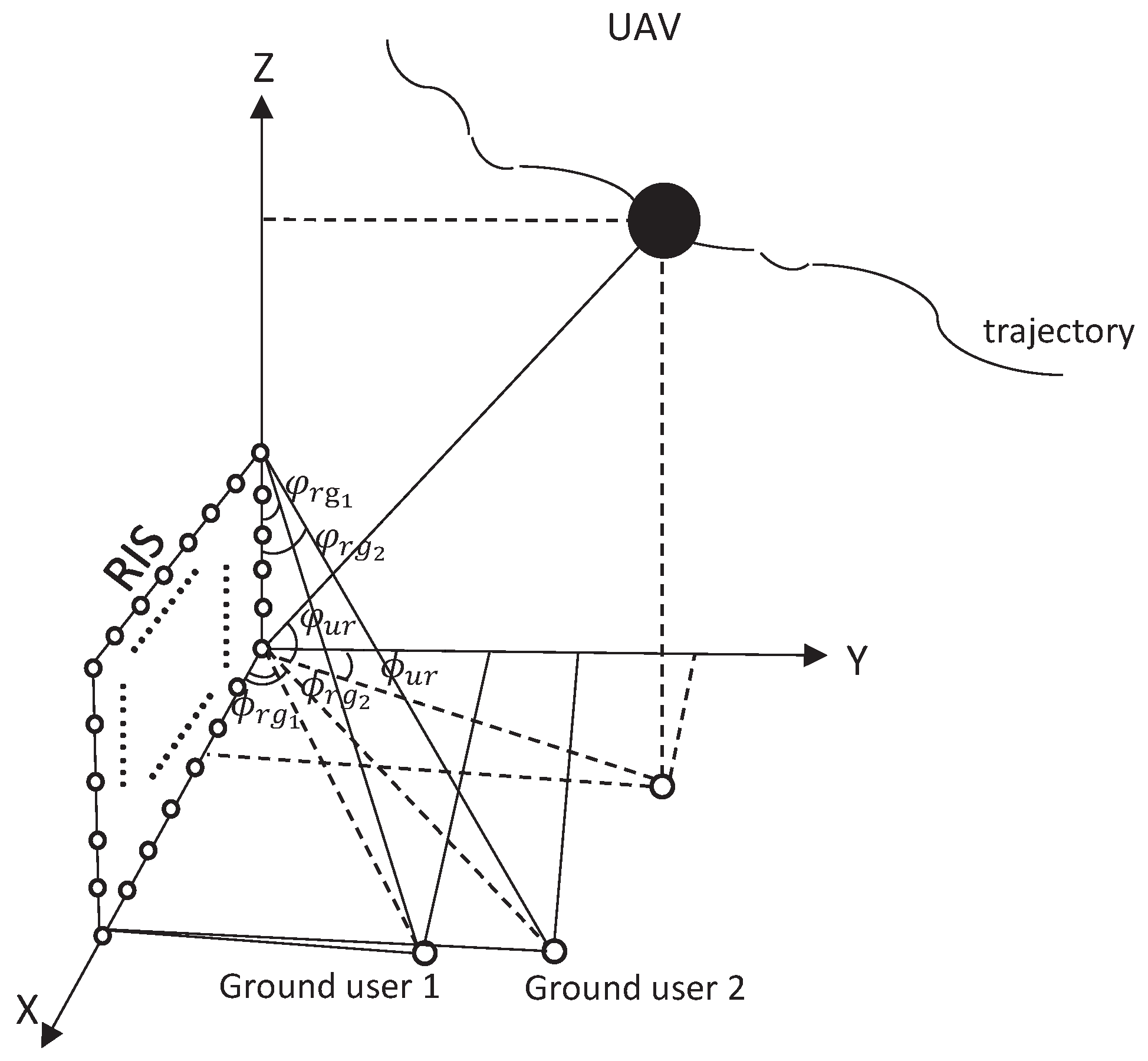
This paper discusses a RIS-assisted NOMA-UAV communication system architecture. The system consists of a UAV in flight, a RIS deployed on a wall, and two ground terminal users utilizing NOMA communication. The UAV maintains a line-of-sight (LoS) wireless connection with the RIS installed on the building’s side wall to ensure stable signal propagation. Even if the wireless connection between the UAV and the terrestrial user is interrupted, the system can still use RIS to enable effective signal reception by the ground user. All nodes involved in the communication process are positioned in a three-dimensional rectangular coordinate system, as shown in
Figure 1. The location of the User 1 is set to
, and the location of the User 2 is set to
. The complete flight path of the UAV is expanded in the X-Y-Z three-dimensional coordinate system. During the whole flight cycle, the flight height of UAV remains unchanged, which is
[
9]. In addition, the height of RIS is set to
, the location of the RIS is set to
. The maximum speed during flight is limited to
. The UAV’s flight cycle is denoted as
J, which is divided into
K time intervals, each of duration
. The UAV can cover a maximum distance in a single time interval, as calculated by
. Based on this, the position of the UAV at time
k can be represented by
,
. To better align with the actual flight trajectory, the UAV follows the constraints outlined below.
Here
and
denote the UAV’s starting and terminal points. The constraint achieves a high-precision dynamic approximation of the real flight trajectory by discretizing the continuous path into a series of differential segments.
The RIS is assumed to consist of a uniform planar array with elements. is defined as a diagonal phase matrix, where denotes the stage value of the th reflection unit in the k slot.
and
are set as the direct links from UAV to ground User 1 and User 2, respectively. Although the direct signal from the transmitting source to the receiver may be blocked by obstacles, some signals can bypass these obstructions through reflection or scattering. These signals will experience attenuation or interference during propagation. A commonly used model to describe this phenomenon is Rayleigh fading. The values of
and
in the
kth time slot can get
and
are the distance from UAV to User 1 and User 2 respectively. The
is the path loss, and
is the path loss index of UAV-user.
and
. Assuming that the channel between UAV and RIS is a LoS channel and is set to
, the value of
at the
kth time slot can obtain
the
d represents the interval between the antennas,
represents the wavelength,
is the signal loss index of the UAV-RIS, and
is the distance of the UAV-RIS in the time slot.
,
,
,
and
respectively denote the azimuth and pitch angle of the signal from UAV to RIS within time slot
k.
We define the distance between the user and the RIS as the distance from the user to the first array element of the RIS [
25]. The channel between RIS users is modeled using Rician fading effect. Unlike Rayleigh fading, the Rician model accounts for the reflected signals from the RIS, denoted as
and
. Then
and
can get
we define parameters
and
as the distances from the RIS to User 1 and User 2, which facilitates subsequent performance analysis.
and
represent the circular symmetric complex Gaussian distribution.
is the Rician factor;
is the path loss index corresponding to RIS-ground users. And
, where
,
,
and
signify the horizontal and vertical directions, respectively, of the signal being transmitted from the RIS-ground User 1. Similarly,
, where
,
,
and
represent the horizontal and vertical directions, respectively, of the signal transmitted from the RIS to ground-based User 2. To facilitate subsequent calculations, we transform
and
into
The amplitude and phase are decoupled to simplify the calculation. Where
and
represent the amplitude of each element
of
and
respectively, and
and
represent the phase of each element (m,n) of
and
respectively.
We assume that the signals in the system take the form of linear combinations, with each signal affected by different noises and disturbances. The signal in the system can be expressed as:
, where
y is the received signal,
H is the channel matrix,
s is the transmitted signal, and
n is the noise. To ensure successful decoding, when the signal-to-noise ratio (SNR) of the received signal exceeds the decoding threshold, the receiver can recover the target signal. The residual interference in subsequent signal processing can be significantly reduced by reconstructing and eliminating the interference component. This expresses it as:
where
is the target SNR of the current signal, and
is the minimum SNR required for successful decoding. To minimize the influence of the signal on subsequent processing after decoding, the interference power must be minimized. This can be quantified by the interference-to-noise ratio (INR) of each signal, we can get:
Next, we sort the signal intensities and determine the decoding order. After decoding the interference signal, perfect SIC can be achieved by minimizing the interference power.
In the NOMA system, ground users employ SIC to decode their signals. To streamline the analysis, we posit the sequence of decoding [
26]. We first regard the signal of User 2 as noise to decode the signal of User 1, and then remove it from the superimposed signal. Then you need to meet the following constraints.
and
are the power allocated by the UAV to User 1 and User 2 for transmission in
k time slots, respectively.
and
represent the joint channel vectors of UAV to ground User 1 and ground User 2 at the
kth time slot, respectively.
Then the average achievable rates of User 1 and User 2 take the form of
Then we can obtain the average achievable rate
4. Proposed Algorithm
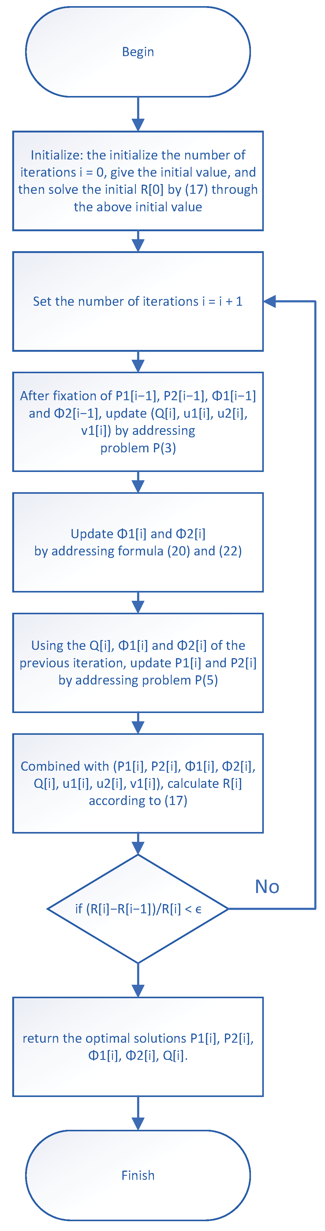
In the previous section, we derive the optimization problem. Due to the presence of coupling variables and non-convex constraints, problem presents a significant challenge. Therefore, we dissect the problem into three distinct sub-problems: the optimization of RIS phase shifts, UAV transmission power, and UAV flight trajectories.
4.1. RIS Phase Shift Optimization
When we fix the UAV power
and UAV flight trajectory
Q, we can rewrite
as
and through the integration of phase can be drawn
. According to [
27], the equivalent maximum channel gain is achieved when the phases of
and
are aligned. Then we can derive it from
Using the same method, we can express the
as
where
. We align the phase of RIS to User 1. According to the literature [
28], we align the RIS phase with User 1, as the positions of User 1 and User 2 differ, resulting in a phase difference. So we make
and put
into
, we can get
Because of mathematical formulae
, we can rewrite
and
as
RIS can be equipped with high-precision phase control modules (e.g., varactor diodes) that independently adjust the phase of each reflection unit. In this paper, an alternating iterative iterative solution method is employed to ensure smooth and continuous phase adjustment, while the UAV’s continuity constraints are incorporated to prevent system instability. Therefore, continuous-phase operation is feasible.
Quantization phase shifts introduce errors that affect the accuracy, stability, and complexity of the optimization problem, particularly at lower quantization levels (e.g., 2-bit and 4-bit), where larger quantization errors can degrade convergence speed and algorithm accuracy. Additionally, lower quantization levels reduce the signal-to-noise ratio and increase the bit error rate, potentially limiting the achievable transmission rate.
This section focuses on UAV trajectory optimization. Following this, we will address the UAV power allocation problem.
4.2. UAV Trajectory Optimization
By fixing the RIS phase shift
and the UAV power
, there is only one variable
Q. Then we can get
both
and
are nonconvex, we will deal with them separately and transform them into convex functions. Expand Formulas (
23) and (
24) to get
where
,
,
,
. In order to relax the constraints, we introduce the relaxation variables
,
and
to strike a balance between the constraint strictness and the problem’s solvability.
Substituting Formulas (
27)–(
29) into Formulas (
25) and (
26), we can get
Taylor approximation is a technique used to approximate a function by utilizing its derivative information at a specific point. Let have all derivatives of order at a point , then the Taylor expansion of at that point is: . This expansion approximates the function value by progressively incorporating higher-order derivatives. In practical applications, the Taylor series is typically truncated to obtain an approximation. The accuracy of the Taylor expansion relies on the local linearization assumption and the differentiability of the function. In this paper, each iteration requires calculating only the gradient at the current point, with the expansion truncated to a single term.
Next, we obtain the first-order Taylor series of
and
for fixed points
and
, respectively. That is, we calculate the first-order partial derivatives of
,
and
for (
32) and (
33). Then we can get
where
,
,
,
,
,
,
,
,
,
. To simplify the equation, symbols are used in place of complex terms.
Finally, we can conclude that the optimization problem
of UAV trajectory can be rewritten as
where
,
. Finally, problem
has the property of convexity. Based on this property, mature standard optimization solvers, such as CVX [
29], can efficiently solve this problem.
4.3. UAV Power Allocation Optimization
When we fix RIS Phase Shift
and UAV flight trajectory
Q. In order to facilitate the distinction, the following uses
instead of
,
instead of
. We can rewrite problem
as
The consequence of adding two functions with convexity is still a convex-type function [
30]. The non-convex component of problem
is
, which primarily transforms
into a convex function. Based on the properties of logarithms, the division of logarithms with the same base can be rewritten as the difference of two logarithms. Convert
into
The latter term of the above equation is expanded by the first-order Taylor expansion at the fixed point
, while the former term remains unchanged. We can get
we can solve
directly. We can rewrite problem
as
Since problem
features a linear objective function coupled with linear inequality constraints, its convexity can be easily proven. Thus, the transformed problem
can be solved by using the CVX [
29] tool.
6. Numerical Results
The following are the settings for the simulation parameters. The ground users is located at and , respectively. And the RIS is positioned at , with the RIS standing at a height of m. For the UAV, its flight altitude remains constant at m, starting from the position and concluding its journey at . The parameter settings are as follows: In the current configuration, both the ground users and the UAV each have one antenna. The Rician factor is dB. The remaining parameter settings are m/s, dB, , s, , , , , mw, dBm. For Algorithm 1, the threshold value of is established at . We set the maximum number of iterations to 20.
We demonstrate the simulation findings acquired through implementing our devised algorithm (abbreviated as OT&OP&OW). For the purpose of comparative analysis, we introduce three additional benchmark algorithms. The trajectory optimization design that also optimizes phase shifts (abbreviated as OT&OP), aiming to find the optimal trajectory while considering phase-shift optimization. The initial trajectory design that optimizes phase shifts (abbreviated as T&OP), aiming to enhance signal performance through phase adjustment. The power optimization design with optimized phase shifts (abbreviated as OW&OP), which focuses on optimizing power allocation while adjusting phase shifts. The initial trajectory design based on random phase (abbreviated as T&RP), where the phase values are randomly assigned. If the duration is sufficiently long, the UAV follows the initially planned trajectory. However, if the available time is limited, the UAV will deviate from the set trajectory and proceed directly to the endpoint at maximum speed.
Initial feasible solutions for the OT&OP&OW, OT&OP, and OW&OP algorithms are generated using the T&RP algorithm. These initial solutions act as a starting point for further optimization. During the flight cycle, the initial power values for these algorithms are randomly generated, with the condition that the power of exceeds that of .
In
Figure 2, we look at the UAV’s initial trajectory and optimized trajectories, with number of array elements
M varying. This helps us see how
M impacts the UAV’s flight path. The UAV initially chooses to hover over User 2 to achieve the maximum average rate and flies directly to User 2. As the quantity of RIS array elements rises, the UAV’s trajectory bends and gradually shifts towards the RIS position in the middle. When the RIS array elements are sufficient, the UAV will hover between RIS and User 2.
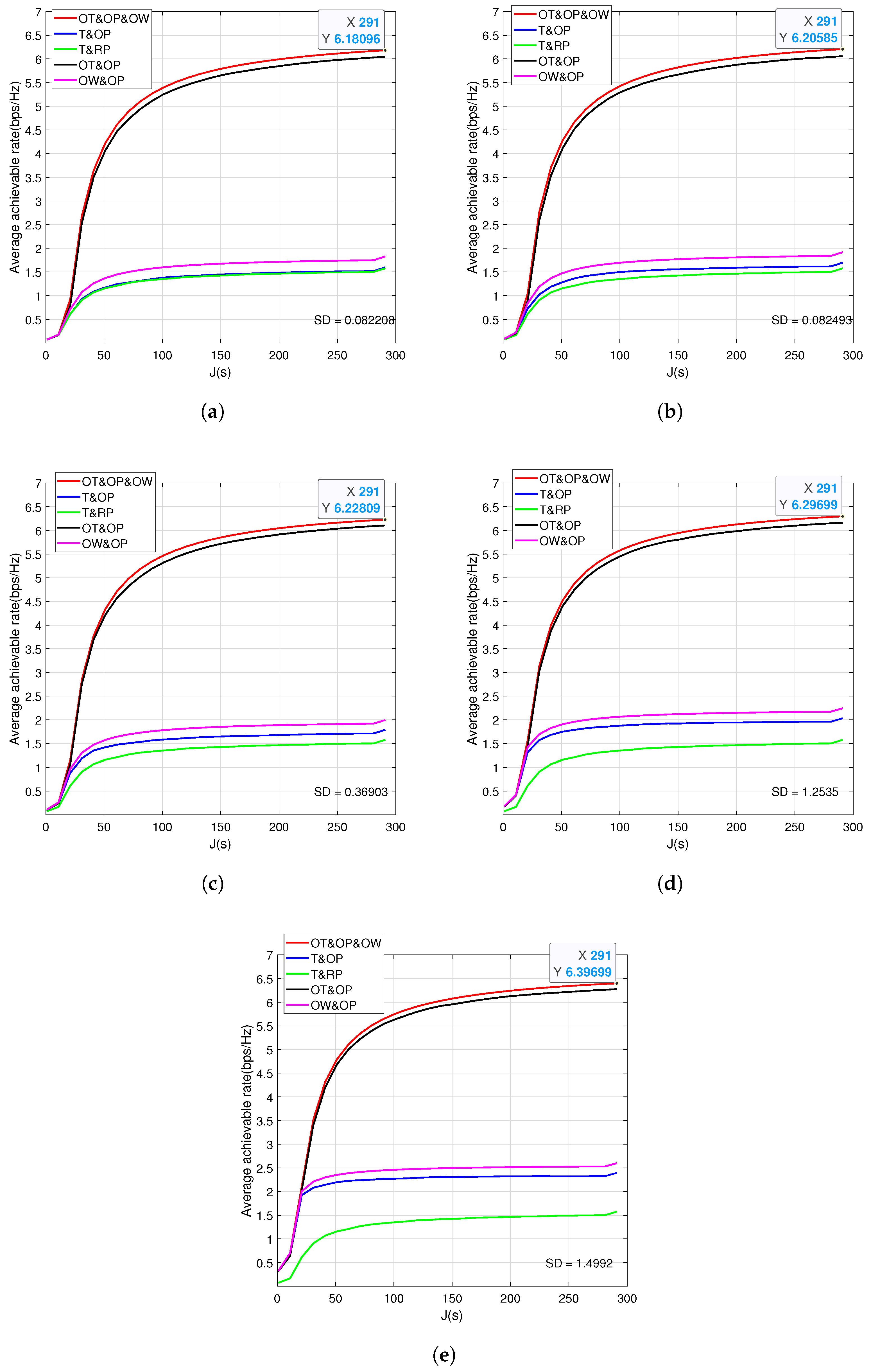
In
Figure 3, we illustrate the bearing of different RIS array elements on the average achievable rate under the same maximum transmit power. We use the standard deviation (denoted as SD) as a measure of data dispersion. As RIS array elements increases, the degree of dispersion also increases. As the number of RIS array elements increases, the overall optimization effect shows minimal improvement. However, the blue and pink curves reveal a significant increase in phase optimization as the number of RIS elements grows. Combined with
Figure 2, since the UAV trajectory is not close to the RIS, the impact of adding more RIS array elements on the overall performance is minimal. However, it can be concluded that even with a small number of RIS array elements, our scheme effectively improves the system’s average achievable rate, in contrast to relying on a large number of elements.
In
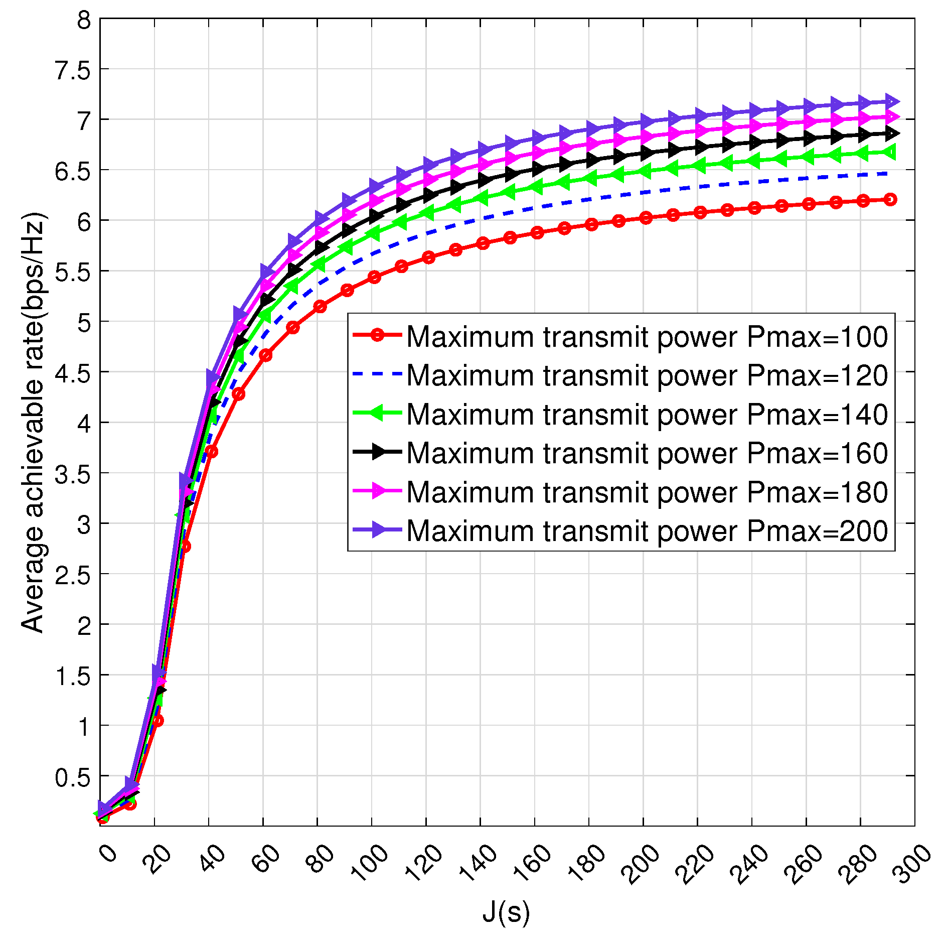
Figure 4, we give the influence of different peak transmission power
on the average achievable rate under the same RIS array elements
M. It can be inferred that as
increases, the mean achievable throughput also increases significantly. Since the UAV’s flight trajectory hovered over User 2, increasing
had a minimal impact on overall optimization. This suggests that increasing
yields a better optimization effect compared to increasing the RIS array elements. Considering the RIS layout and installation cost, the choice of increasing
is a better choice.
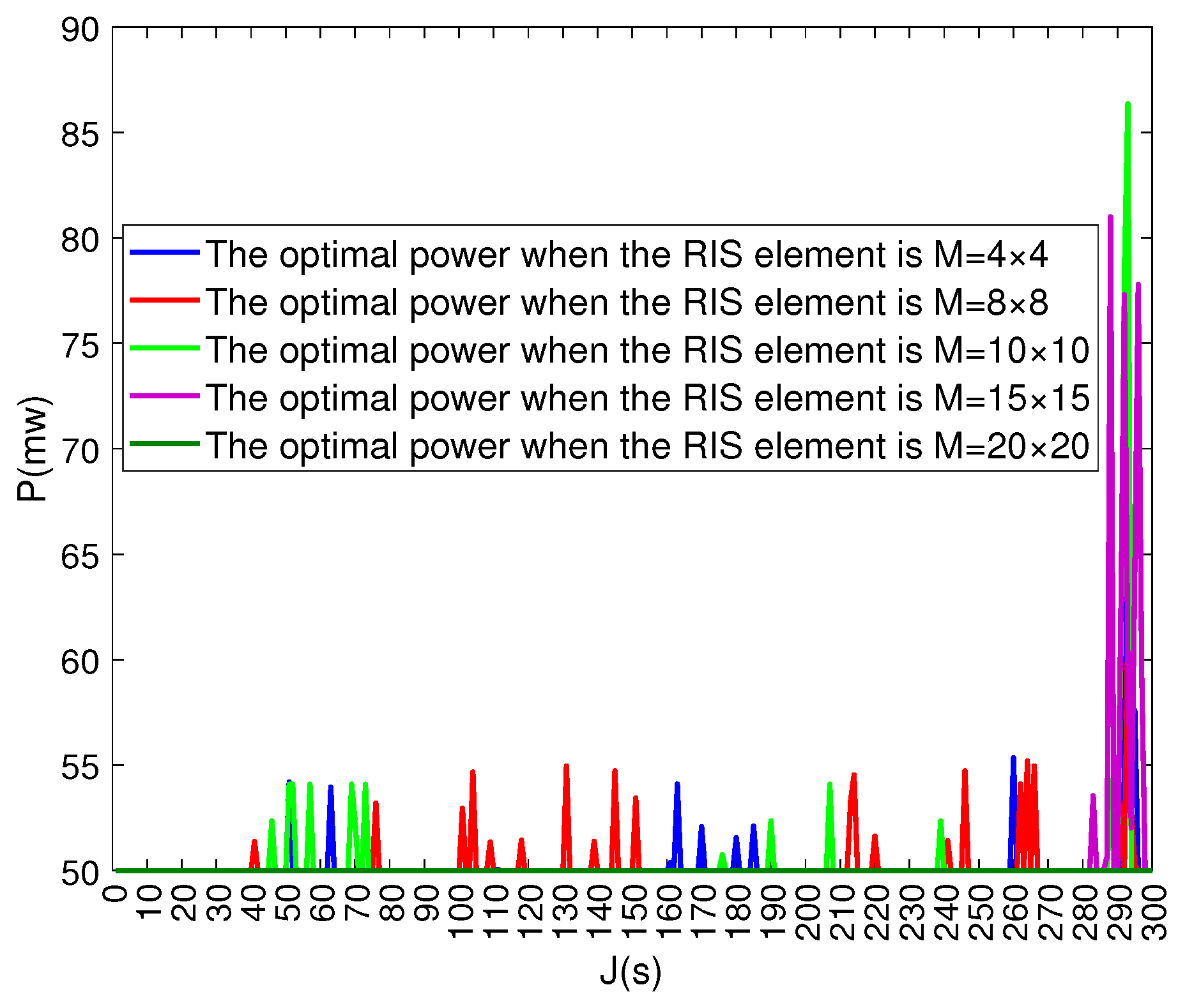
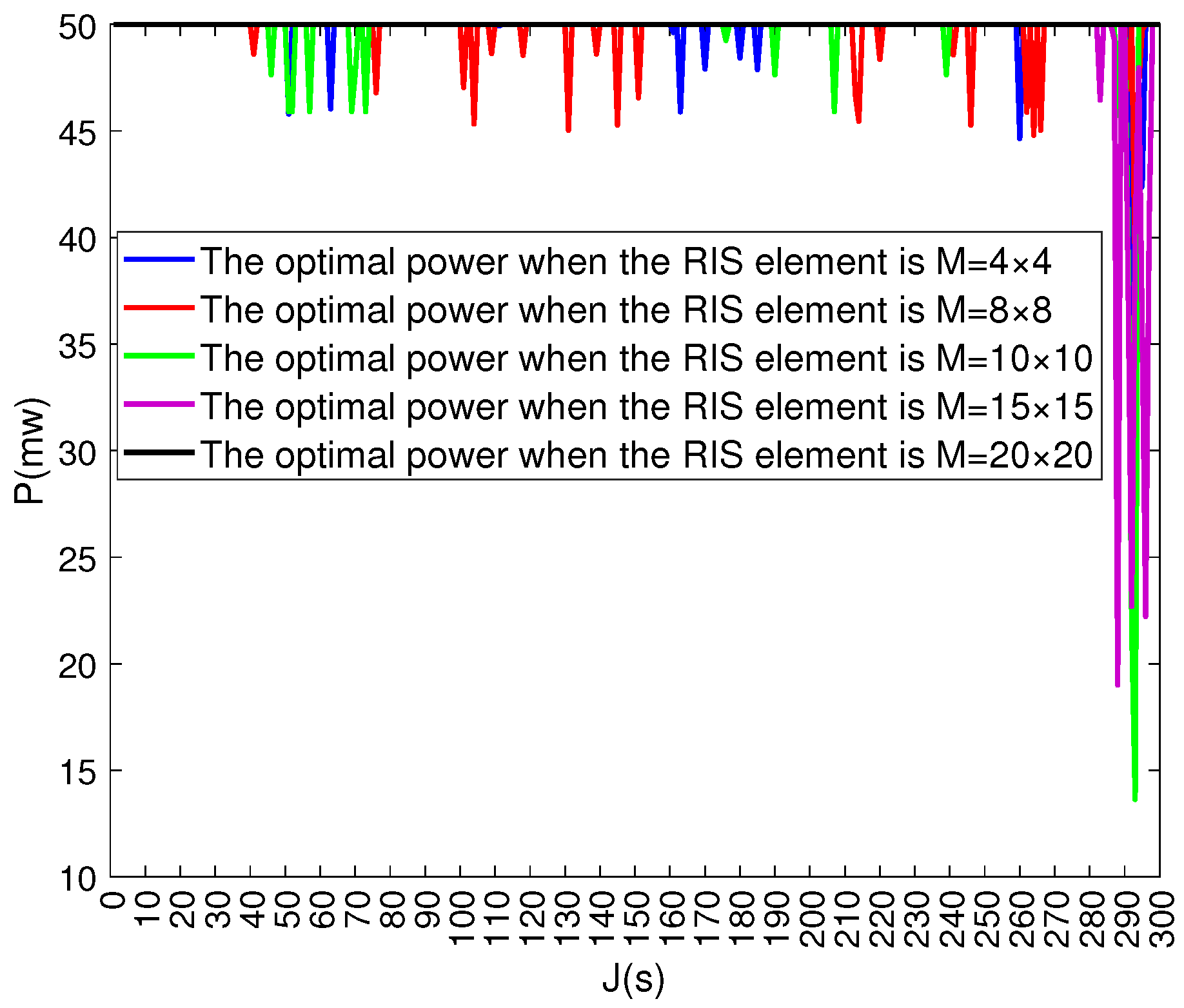
Figure 5 and
Figure 6 are in the same
, the influence of different
M on the mean achievable throughput. It can be observed that both
and
fluctuate around 50 mW, while 50 mW remains stable without fluctuation. The power allocated to both components satisfies the constraints. The maximum average achievable rate is obtained based on atransmission power allocation during the flight. As the number of RIS array elements increases, the fluctuation becomes smaller. When the RIS array element is
, the power allocated to both users is 50 mw, and the UAV trajectory is closer to the RIS. At certain times, the UAV allocates more power to User 1 and less to User 2 to ensure both users achieve a higher communication rate.


