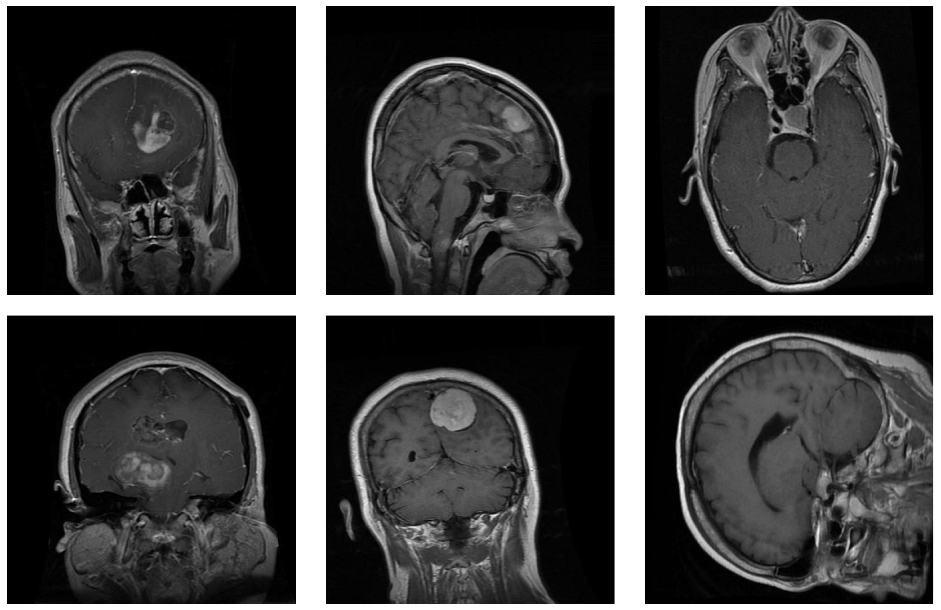
Figure 1.
Samples from the brain dataset: the first column shows two examples of glioma tumors; the middle column shows meningioma tumors; and the last column depicts images of pituitary tumors.
Figure 1.
Samples from the brain dataset: the first column shows two examples of glioma tumors; the middle column shows meningioma tumors; and the last column depicts images of pituitary tumors.
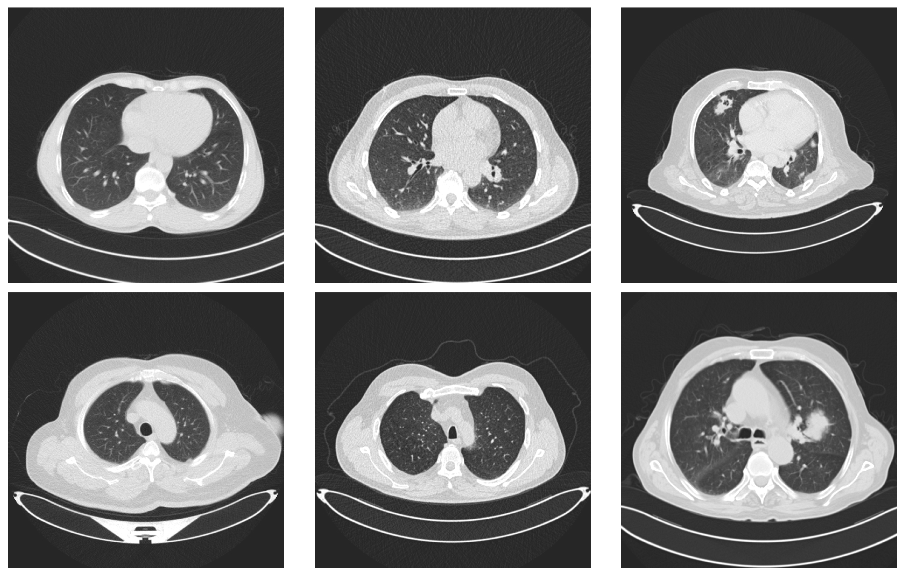
Figure 2.
Examples of lung images. Images in the first column represent lungs with no tumors. The images in the middle column represent benign tumors and the last column contains two images with malignant tumors.
Figure 2.
Examples of lung images. Images in the first column represent lungs with no tumors. The images in the middle column represent benign tumors and the last column contains two images with malignant tumors.
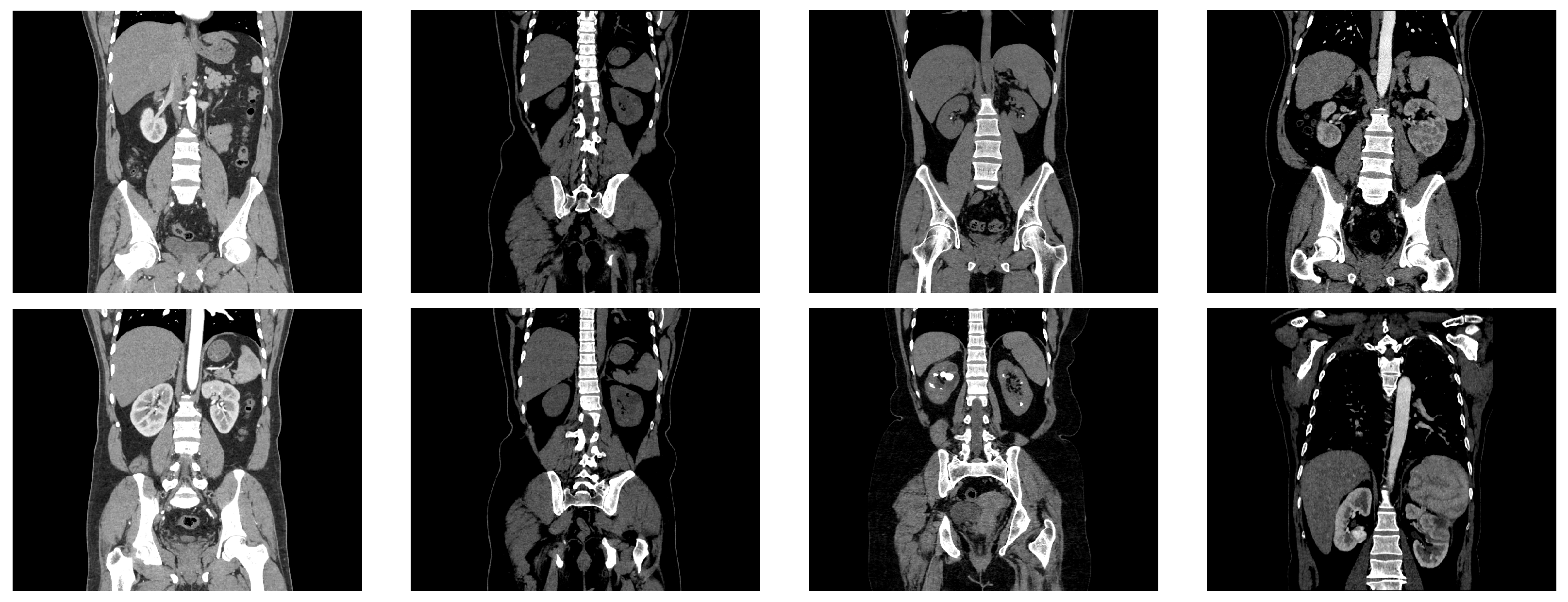
Figure 3.
Examples from the kidney dataset. The two images in the first column represent CT images of normal kidneys, the two images in the second column depict kidneys with cysts, the images in the third column represent CT images of kidneys with stones, and the images in the last column depict kidneys with cancer.
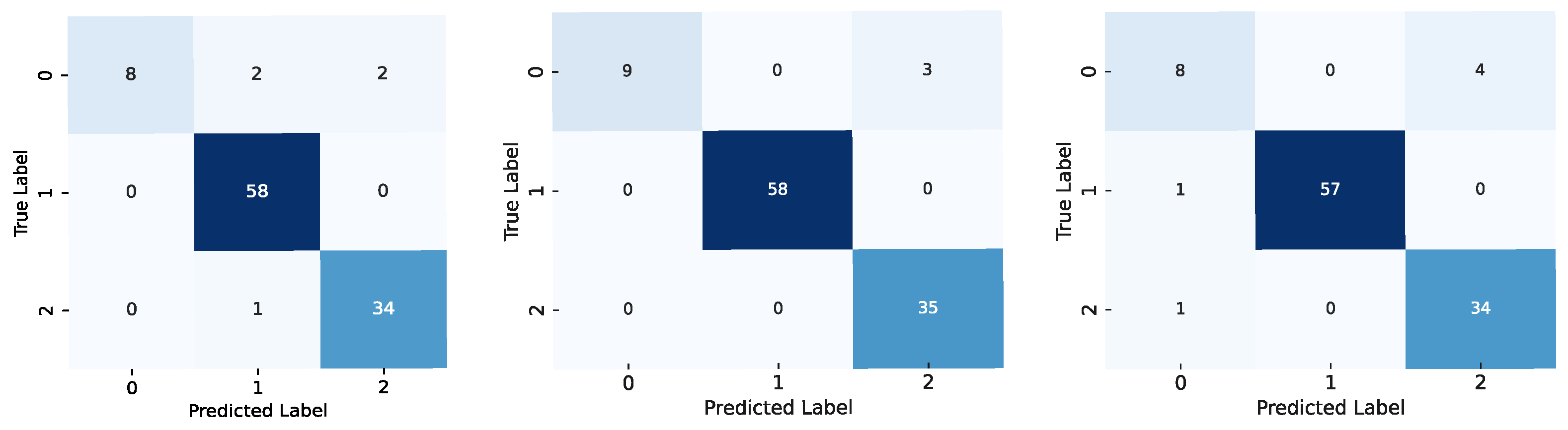
Figure 4.
Confusion matrices for the models using the brain dataset: results for the ViT-b-32 model are on the left, those for the Swin-t model are in the middle, and those for the MaxViT-t model are on the right. The label codes are glioma (0), meningioma (1), and pituitary (2).
Figure 4.
Confusion matrices for the models using the brain dataset: results for the ViT-b-32 model are on the left, those for the Swin-t model are in the middle, and those for the MaxViT-t model are on the right. The label codes are glioma (0), meningioma (1), and pituitary (2).
Figure 5.
Confusion matrices for the models using the kidney dataset: results for the ViT-b-32 model are on the left, those for the Swin-t model are in the middle, and those for the MaxViT-t model are on the right. The label codes are cyst (0), normal (1), stone (2), and tumor (3).
Figure 5.
Confusion matrices for the models using the kidney dataset: results for the ViT-b-32 model are on the left, those for the Swin-t model are in the middle, and those for the MaxViT-t model are on the right. The label codes are cyst (0), normal (1), stone (2), and tumor (3).
Figure 6.
Confusion matrices for the models using the lung dataset: results for the ViT-b-32 model are on the left, those for the Swin-t model are in the middle, and those for the MaxViT-t model are on the right. The label codes are benign (0), malignant (1), and normal (2).
Figure 6.
Confusion matrices for the models using the lung dataset: results for the ViT-b-32 model are on the left, those for the Swin-t model are in the middle, and those for the MaxViT-t model are on the right. The label codes are benign (0), malignant (1), and normal (2).
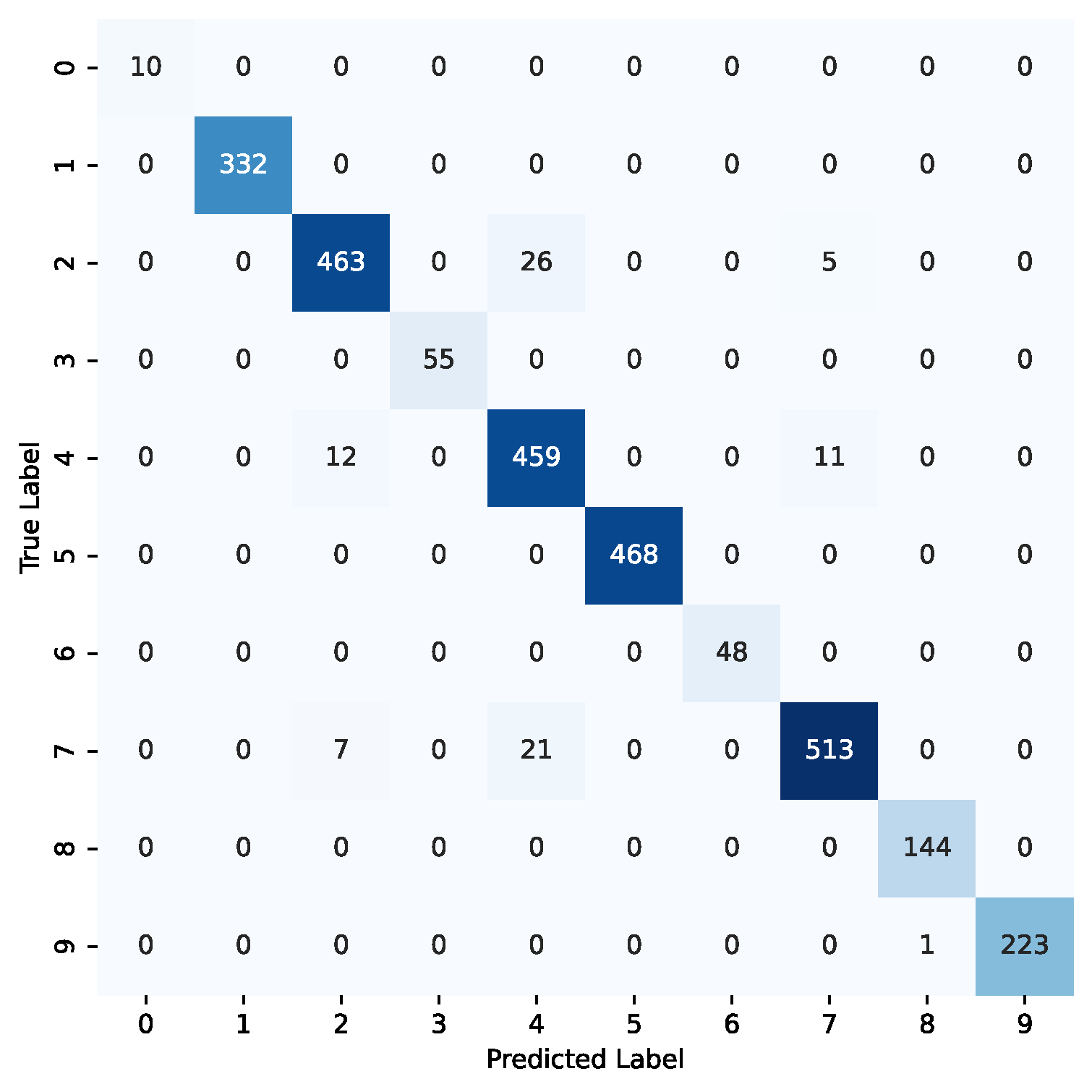
Figure 7.
Confusion matrix for the ViT-32-b model using the combined datasets. The label codes are as follows: benign (0—lung), cyst (1—kidney), glioma (2—brain), malignant (3—lung), meningioma (4—brain), normal (5—kidney), normal (6—lung), pituitary (7—brain), stone (8—kidney), tumor (9—kidney).
Figure 7.
Confusion matrix for the ViT-32-b model using the combined datasets. The label codes are as follows: benign (0—lung), cyst (1—kidney), glioma (2—brain), malignant (3—lung), meningioma (4—brain), normal (5—kidney), normal (6—lung), pituitary (7—brain), stone (8—kidney), tumor (9—kidney).
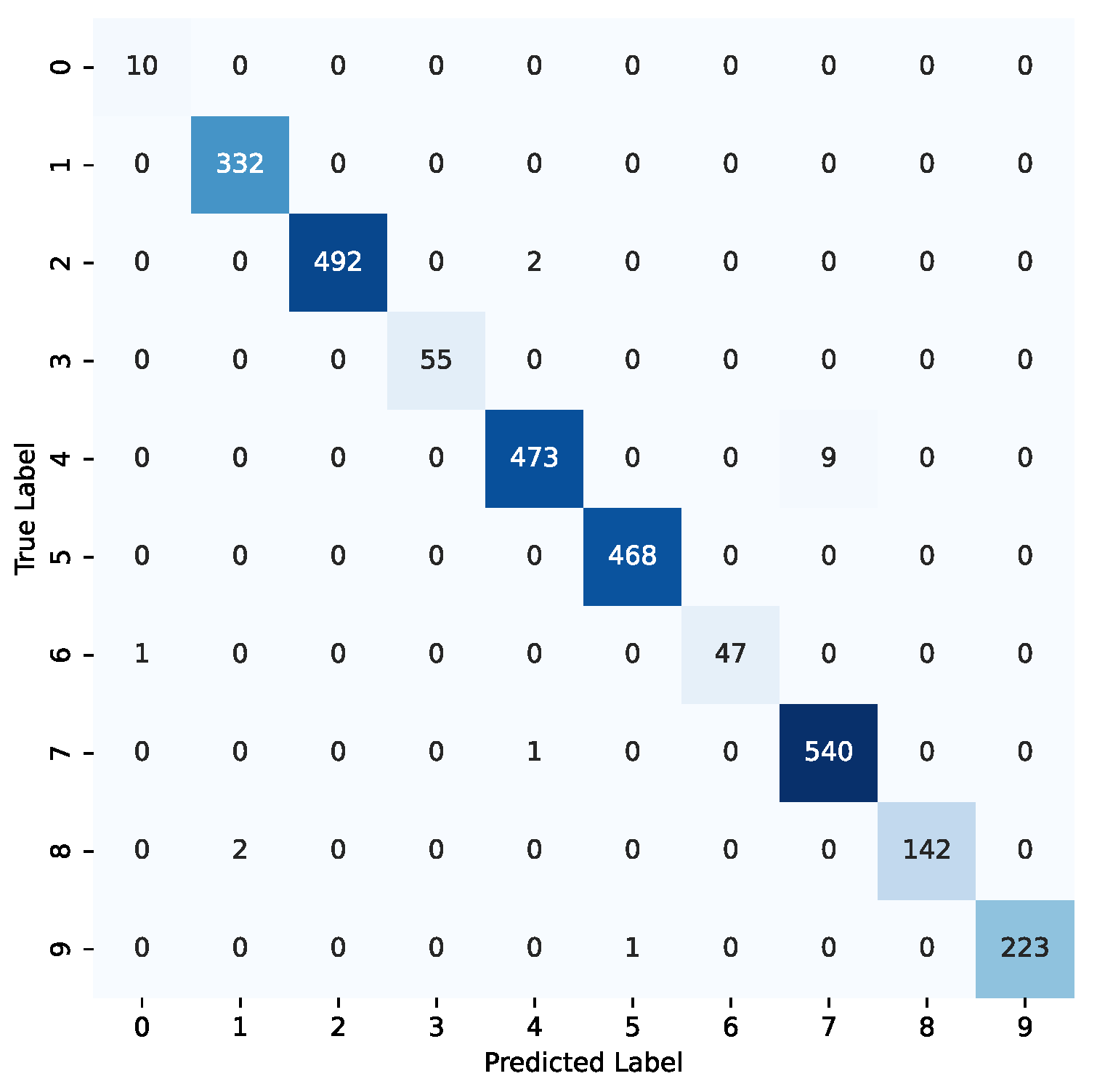
Figure 8.
Confusion matrix for the Swin-t model using the combined datasets. The label codes are as follows: benign (0—lung), cyst (1—kidney), glioma (2—brain), malignant (3—lung), meningioma (4—brain), normal (5—kidney), normal (6—lung), pituitary (7—brain), stone (8—kidney), tumor (9—kidney).
Figure 8.
Confusion matrix for the Swin-t model using the combined datasets. The label codes are as follows: benign (0—lung), cyst (1—kidney), glioma (2—brain), malignant (3—lung), meningioma (4—brain), normal (5—kidney), normal (6—lung), pituitary (7—brain), stone (8—kidney), tumor (9—kidney).
Figure 9.
Confusion matrix for the MaxViT-t model using the combined datasets. The label codes are as follows: benign (0—lung), cyst (1—kidney), glioma (2—brain), malignant (3—lung), meningioma (4—brain), normal (5—kidney), normal (6—lung), pituitary (7—brain), stone (8—kidney), tumor (9—kidney).
Figure 9.
Confusion matrix for the MaxViT-t model using the combined datasets. The label codes are as follows: benign (0—lung), cyst (1—kidney), glioma (2—brain), malignant (3—lung), meningioma (4—brain), normal (5—kidney), normal (6—lung), pituitary (7—brain), stone (8—kidney), tumor (9—kidney).
Table 1.
Distribution of samples in the lung dataset. For each type of class, this table shows the number of cases in the second column and the number of images in the third column.
Table 1.
Distribution of samples in the lung dataset. For each type of class, this table shows the number of cases in the second column and the number of images in the third column.
| Type | Images |
|---|
| Healthy Lung | 405 |
| Benign Tumor Lung | 102 |
| Cancerous Tumor Lung | 547 |
Table 2.
Distribution of samples in the classes of the kidney dataset.
Table 2.
Distribution of samples in the classes of the kidney dataset.
| Class | Number of Images |
|---|
| Normal | 5002 |
| Cyst | 3284 |
| Stone | 1360 |
| Cancer | 2283 |
Table 3.
Details of different variants of the ViT model.
Table 3.
Details of different variants of the ViT model.
| Model | Layers | Hidden Layers | MLP Size | Heads | Parameters (in Millions) |
|---|
| ViT-Base | 12 | 768 | 3072 | 12 | 86 |
| ViT-Large | 24 | 1024 | 4096 | 16 | 307 |
| ViT-Huge | 32 | 1280 | 5120 | 16 | 632 |
Table 4.
Complexity of the models.
Table 4.
Complexity of the models.
| Models | Number of Parameters | FLOPS (Millions) | Size (Megabytes) |
|---|
| ViT-b-32 | 88,185,064 | 456.96 | 344.59 |
| Swin-t | 28,288,354 | 123.43 | 141.22 |
| MaxViT-t | 30,919,624 | 5600.0 | 118.80 |
Table 5.
Accuracy of the models after the first transfer learning step. This table shows the accuracy of the models for each dataset. The last row depicts the results of each model by combining the three datasets. Bold letters highlight the best results in each row.
Table 5.
Accuracy of the models after the first transfer learning step. This table shows the accuracy of the models for each dataset. The last row depicts the results of each model by combining the three datasets. Bold letters highlight the best results in each row.
| Dataset | ViT-b-32 | Swin-t | MaxViT-t |
|---|
| Brain | 93.27% | 93.07% | 91.47% |
| Kidney | 97.15% | 95.55% | 88.51% |
| Lung | 93.33% | 90.48% | 87.62% |
| All datasets | 95.43% | 93.82% | 83.60% |
Table 6.
Accuracy of the models using transfer learning. This table shows the accuracy of ViT-b-32, Swin-t, and MaxViT-t for each dataset. The last row depicts the results of each model by combining the three datasets. Bold letters highlight the best results in each row.
Table 6.
Accuracy of the models using transfer learning. This table shows the accuracy of ViT-b-32, Swin-t, and MaxViT-t for each dataset. The last row depicts the results of each model by combining the three datasets. Bold letters highlight the best results in each row.
| Dataset | ViT-b-32 | Swin-t | MaxViT-t |
|---|
| Brain | 97.07% | 99.53% | 99.27% |
| Kidney | 97.73% | 99.75% | 99.75% |
| Lung | 95.24% | 97.14% | 94.29% |
| All datasets | 97.03% | 99.43% | 98.68% |
Table 7.
Performance assessment for the brain dataset: the first column shows the model used in each experiment; the second column depicts the accuracy of the model for the test set; the third column shows the training time in seconds per epoch; the forth column shows the inference time in milliseconds per image; the fifth column shows the number (#) of parameters of each network; and the last column shows the number of FLOPS. The last two columns are copied from
Table 4.
| Model | Accuracy | Training Time | Inference Time | #Parameters | FLOPS (Mill) |
|---|
| ViT-b-32 | 97.07% | 87 s/epoch | 5.8 ms/image | 88,185,064 | 456.96 |
| Swin-t | 99.53% | 142 s/epoch | 16.7 ms/image | 28,288,354 | 123.43 |
| MaxViT-t | 99.27% | 155 s/epoch | 41.3 ms/image | 30,919,624 | 5600.0 |
Table 8.
Performance of the models for the brain dataset. Bold letters indicate the best result in each metric.
Table 8.
Performance of the models for the brain dataset. Bold letters indicate the best result in each metric.
| Model | Accuracy (%) | Precision | Recall | F1-Score | AUC-ROC |
|---|
| ViT-b-32 | 97.07 | 0.971 | 0.971 | 0.971 | 0.998 |
| Swin-t | 99.53 | 0.995 | 0.996 | 0.995 | 1.0 |
| MaxViT-t | 99.27 | 0.993 | 0.993 | 0.993 | 1.0 |
Table 9.
Performance of the models for the kidney dataset. Bold letters indicate the best result in each metric.
Table 9.
Performance of the models for the kidney dataset. Bold letters indicate the best result in each metric.
| Model | Accuracy (%) | Precision | Recall | F1-Score | AUC-ROC |
|---|
| ViT-b-32 | 97.73 | 0.983 | 0.964 | 0.972 | 0.997 |
| Swin-t | 99.75 | 0.997 | 0.996 | 0.996 | 1.0 |
| MaxViT-t | 99.75 | 0.998 | 0.995 | 0.996 | 1.0 |
Table 10.
Performance of the models for the lung dataset. Bold letters indicate the best result in each metric.
Table 10.
Performance of the models for the lung dataset. Bold letters indicate the best result in each metric.
| Model | Accuracy (%) | Precision | Recall | F1-Score | AUC-ROC |
|---|
| ViT-b-32 | 95.24 | 0.965 | 0.879 | 0.911 | 0.982 |
| Swin-t | 97.14 | 0.974 | 0.917 | 0.939 | 0.993 |
| MaxViT-t | 94.29 | 0.898 | 0.874 | 0.883 | 0.979 |
Table 11.
Performance of the models when we combined all the datasets. Bold letters indicate the best result in each metric.
Table 11.
Performance of the models when we combined all the datasets. Bold letters indicate the best result in each metric.
| Model | Accuracy (%) | Precision | Recall | F1-Score | AUC-ROC |
|---|
| ViT-b-32 | 97.03 | 0.983 | 0.983 | 0.983 | 0.999 |
| Swin-t | 99.43 | 0.988 | 0.994 | 0.991 | 1.00 |
| MaxViT-t | 98.68 | 0.974 | 0.984 | 0.978 | 1.00 |
Table 12.
Comparison of the performance of the models when trained with individual and combined datasets. The results of the individual datasets from the previous tables were averaged (avg). Bold letters indicate the best result in each metric.
Table 12.
Comparison of the performance of the models when trained with individual and combined datasets. The results of the individual datasets from the previous tables were averaged (avg). Bold letters indicate the best result in each metric.
| Model | Accuracy (%) | Precision | Recall | F1-Score | AUC-ROC |
|---|
| ViT-b-32 Individual (avg) | 96.77 | 0.975 | 0.949 | 0.959 | 0.994 |
| ViT-b-32 Combined | 97.03 | 0.983 | 0.983 | 0.983 | 0.999 |
| Swin-t Individual (avg) | 98.96 | 0.988 | 0.975 | 0.980 | 0.998 |
| Swin-t Combined | 99.43 | 0.988 | 0.994 | 0.991 | 1.00 |
| MaxViT-t Individual (avg) | 97.99 | 0.966 | 0.961 | 0.962 | 0.995 |
| MaxViT-t Combined | 98.68 | 0.974 | 0.984 | 0.978 | 1.00 |
Table 13.
Per-class evaluation metrics for the Swin-t model on the combined dataset, including precision, recall, and F1-score for each of the 10 classes. The results highlight the model’s robustness across both majority and minority classes, with strong performance even in low-support categories such as benign and malignant lung tumors.
| Dataset | Class | Precision | Recall | F1-Score |
|---|
| Brain | Glioma | 1.000 | 0.996 | 0.998 |
| Meningioma | 0.995 | 0.981 | 0.988 |
| Pituitary | 0.984 | 0.998 | 0.991 |
| Kidney | Cyst | 0.991 | 1.000 | 0.996 |
| Normal | 0.998 | 1.000 | 0.999 |
| Stone | 0.993 | 0.986 | 0.989 |
| Tumor | 1.000 | 0.995 | 0.997 |
| Lung | Benign | 0.909 | 1.000 | 0.952 |
| Malignant | 1.000 | 1.000 | 1.000 |
| Normal | 1.000 | 0.979 | 0.989 |
Table 14.
Comparison with state-of-the-art methods using similar datasets. The table compares the accuracy of prior works with the results of the Swin-t model. These are represented in bold letters.
Table 14.
Comparison with state-of-the-art methods using similar datasets. The table compares the accuracy of prior works with the results of the Swin-t model. These are represented in bold letters.
| Dataset | Method | Year | Techniques | Accuracy |
|---|
| Brain | Reddy et al. [51] | 2024 | ViT (FTVT-L16) | 98.70% |
| Ishaq et al. [52] | 2025 | Improved EfficientNet | 98.60% |
| Our result | 2025 | Swin Transformer | 99.53% |
| Kidney | Bingol et al. [53] | 2023 | Hybrid CNN (Relief + WNN) | 99.37% |
| Pimpalkar et al. [54] | 2025 | InceptionV3 CNN | 99.96% |
| Our result | 2025 | Swin Transformer | 99.75% |
| Lung | Pathan et al. [55] | 2024 | Optimized CNN with SCA | 99.00% |
| Jian et al. [56] | 2025 | CNN + GRU | 99.77% |
| Our result | 2025 | Swin Transformer | 97.14% |


