KAN-Sense: Keypad Input Recognition via CSI Feature Clustering and KAN-Based Classifier

Abstract

Wi-Fi sensing leverages variations in CSI (channel state information) to infer human activities in a contactless and low-cost manner, with growing applications in smart homes, healthcare, and security. While deep learning has advanced macro-motion sensing tasks, micro-motion sensing such as keypad stroke recognition remains underexplored due to subtle inter-class CSI variations and significant intra-class variance. These challenges make it difficult for existing deep learning models typically relying on fully connected MLPs to accurately recognize keypad inputs. To address the issue, we propose a novel approach that combines a discriminative feature extractor with a Kolmogorov–Arnold Network (KAN)-based classifier. The combined model is trained to reduce intra-class variability by clustering features around class-specific centers. The KAN classifier learns nonlinear spline functions to efficiently delineate the complex decision boundaries between different keypad inputs with fewer parameters. To validate our method, we collect a CSI dataset with low-cost Wi-Fi devices (ESP8266 and Raspberry Pi 4) in a real-world keypad sensing environment. Experimental results verify the effectiveness and practicality of our method for keypad input sensing applications in that it outperforms existing approaches in sensing accuracy while requiring fewer parameters.

1. Introduction

Motion sensing has traditionally been achieved using physical sensors, such as wearable devices attached to the human body. While these approaches benefit from stable and reliable measurements, they impose limitations in terms of user comfort, battery maintenance, and risk of loss. As an alternative, camera-based vision systems offer contactless sensing with high recognition accuracy thanks to the advances in deep learning. However, such systems raise serious privacy concerns and suffer from degraded performance under poor lighting or occlusion. In contrast, Wi-Fi sensing is a technology that infers motion changes by analyzing variations in CSI (channel state information) induced by the movements of sensing targets [1,2,3]. Since Wi-Fi signals can penetrate obstacles and function without line of sight, Wi-Fi sensing can provide a contactless, device-free, and privacy-preserving solution. Given these advantages, Wi-Fi sensing has garnered significant attention in a wide range of applications, including smart homes [4], healthcare [5], and security [6]. Recently, the rapid advancement of deep learning techniques has further enhanced the sensing performance of a Wi-Fi-sensing system [7,8].

Although macro-sensing tasks such as presence detection, gait recognition, and activity recognition [9] have been widely studied, research on micro-sensing tasks is still relatively limited. However, since micro-motion sensing, such as detecting keystrokes, finger gestures, and subtle hand movements, has potential to transform everyday interactions in both consumer and security contexts, interest in micro-sensing tasks keeps increasingly growing. For instance, in public terminals and kiosks, where physical contact raises hygiene and maintenance concerns, Wi-Fi-based micro-motion recognition enables users to input commands without touching the screen or keypad. In assistive technology for people with disabilities, it can allow individuals with limited motor functions to interact with digital systems through minimal finger or hand gestures. In smart homes and offices, users can control appliances using finger taps or gestures detected in the air, even when holding objects or wearing gloves [10]. Moreover, in security-sensitive environments, micro-motion sensing provides a new layer of behavioral authentication. Subtle differences in keystroke dynamics or hand motions can uniquely identify individuals, complementing conventional password or biometric authentication. This opens up possibilities for continuous, passive user identification based on everyday interaction patterns without requiring explicit input. These compelling use cases highlight the increasing demand for Wi-Fi-based micro-motion sensing. However, compared to macro-motion sensing, micro-motion sensing targets subtle movements. Therefore, there is an inherent difficulty in distinguishing between sensing classes with subtle Wi-Fi signal variations. Moreover, the variability of measured CSI and the structural limitations of conventional deep learning models pose challenges to achieving high sensing accuracy in micro-motion scenarios. Therefore, resolving the associated challenges is of urgent importance.

Deep learning-based Wi-Fi sensing models typically consist of two main components: a feature extractor that derives meaningful representations from the measured Wi-Fi signal data and a classifier that distinguishes these features across different sensing classes. Since both components are trained in an end-to-end manner under the same loss function, addressing the challenges associated with each in a unified framework is crucial for enhancing sensing accuracy. Because the magnitude of movement involved in keypad input sensing is very small, the differences among CSI measurements belonging to different classes are inherently subtle. Furthermore, even when the same individual presses the same key on a keypad, slight variations in motion and positioning can lead to significant differences in the resulting measurements. These inconsistencies cause a large intra-class variance in the feature space, which increases the likelihood that the distributions of CSI features corresponding to different keystrokes will overlap. As a result, it becomes more difficult for the classifier to establish clear decision boundaries between classes, thereby elevating the probability of sensing errors. In deep learning models for Wi-Fi sensing, a wide range of techniques has been employed for feature extraction, including convolutional layers, attention mechanisms, residual networks, and recurrent layers [8]. However, the classifier component has predominantly relied on fully connected multi-layer perceptron (MLPs). MLPs are universal function approximators [11]. They approximate classification functions by applying fixed nonlinear activation functions after linear transformations at each layer. Even though they can approximate any function, MLPs are computationally expensive because they employ a fully connected structure in which each neuron is connected to every neuron in the next layer. As a result, a large number of learnable parameters are required to implement an MLP. Therefore, when the input dimensionality is high or the number of neurons in the hidden layers increases, the computational cost grows exponentially. As with other deep learning models, overfitting is one of the challenges in training MLPs. Overfitting may result from multiple causes, such as overly complex architectures with a large number of parameters, limited training data, extended training duration, and structural biases introduced by nonlinear activation functions [12]. To alleviate the risk of overfitting, deep learning models are typically trained with various overfitting mitigation techniques such as early stopping, dropout, and regularization. However, since MLPs generally consist of multiple fully connected layers with nonlinear activation functions, they typically involve a large number of trainable parameters, which increases the risk of overfitting [13]. In addition, the choice of activation functions can influence overfitting. However, since activation functions in MLPs are fixed and not learned during training, MLPs may be overfitted [14,15].

To address these challenges, in this paper, we propose a keypad input sensing method, which is a representative task in the domain of micro-motion sensing. Specifically, we devise a novel approach to both feature learning and classifier design for our keypad input sensing system named as KAN-Sense. In the context of keypad stroke sensing, it is crucial to clearly delineate the boundaries between different keypad classes in the feature space. To this end, we propose a training strategy for the feature extractor that encourages the CSI features corresponding to the same keypad class to be clustered tightly around a class-specific center despite variations in their measurement patterns. This approach enables the feature extractor to better learn discriminative features, thereby allowing the classifier to more effectively distinguish Wi-Fi signal measurements belonging to different classes. To enhance the performance of the MLP classifier, we take advantage of the Kolmogorov–Arnold Network (KAN) [16]. Unlike MLPs, which rely on linear transformations followed by fixed nonlinear activations, the KAN approximates the classification function by directly learning nonlinear transformations in the form of spline functions. This functional representation allows KAN-based classifiers to model complex decision boundaries in a low-dimensional space. Consequently, compared to MLPs, the KAN-based classifier significantly reduces the number of trainable parameters required for accurate classification, improves learning efficiency, and mitigates the risk of overfitting.

To quantitatively evaluate the effectiveness of the proposed method, we construct a Wi-Fi signal measurement environment using commodity Wi-Fi devices compliant with the IEEE 802.11n standard. To collect CSI data, we configure an ESP8266 module with a single transmitting antenna as a transmitter, which sends Wi-Fi frames every 10 ms. A Raspberry Pi 4 equipped with a single receiving antenna and the Nexmon CSI tool is used to capture the channel state information whenever the transmitter sends a frame. Ten people participated in the data collection process by performing keypad stroke actions. Using the collected CSI dataset, we compare the sensing accuracy of conventional deep learning-based Wi-Fi sensing models with that of the proposed method. The experimental results demonstrate that the proposed method outperforms existing approaches by enhancing sensing performance even with fewer model parameters and regardless of the amount of measurement data.

The rest of this paper is organized as follows. In Section 2, we discuss the related works. We present our Wi-Fi keypad sensing system called KAN-Sense in Section 3. Through experiments, we verify the proposed method in Section 4. In Section 5, we conclude the paper with future research directions.

2. Related Works

2.1. Gesture Recognition via Wi-Fi Sensing

The problem of recognizing gestures through channel state information analysis has been assigned as a multi-class classification task, where each class represents a distinct gesture to be recognized. Early studies on CSI-based gesture recognition primarily rely on handcrafted feature extraction and statistical classification models based on conventional machine learning methods. These approaches typically utilize domain knowledge and signal processing techniques to manually design features, which are then classified using algorithms such as SVMs (Support Vector Machines), GMMs (Gaussian Mixture Models), and DTW (Dynamic Time Warping). For instance, the method in [17] extracts statistical features such as mean, variance, root mean square, and power spectral entropy from both amplitude and phase information in the time and frequency domains. These features are then selected using a PCA-based method and classified by a stacked SVM. In [18], CSI sequences from multiple antennas are processed using SVD (Singular Value Decomposition) to extract representative features, which are separately trained using GMMs in both time and frequency domains and fused by fuzzy logic for final classification. In [19], gesture recognition is achieved by modeling CSI variations based on Fresnel zone theory and their relation to user location. Similarly, the authors in [20] apply DWT (Discrete Wavelet Transform) to feature vectors formed by grouping subcarriers to preserve multi-scale information. The system then uses DTW to compute the similarity between input features and the stored templates for classification. The authors in [21] also use DTW-based template matching by storing CSI sequences corresponding to specific events as templates. These traditional approaches are simple and intuitive. Even though they may achieve effective performance with relatively small amounts of data, their performance is limited because conventional methods are not sophisticated enough to capture the subtle class-specific variations present in CSI data.

To address the limitation, deep learning-based approaches have recently garnered significant attention due to their capacity to learn robust and discriminative representations in complex and dynamic environments. In contrast, recent advancements have increasingly focused on deep learning-based methods that automatically learn discriminative representations from raw CSI data. For example, in [22], CSI sequences are transformed into 2D image representations. Then, a sensing method is proposed that integrates ResNet-18 with spatial and channel attention modules to simultaneously recognize gestures and users. This architecture is designed to effectively extract salient information under diverse scenarios. In [23], a 3D CNN is employed to extract spatio-temporal features from CSI-based speed profiles, and a meta-learning-based relation network is used to measure the similarity between support samples and inputs. Thereby, the sensing method enhances generalization to unseen classes or users. The authors in [24] convert CSI data into spectrograms and use an Inception-based CNN to simultaneously capture features across various receptive fields for efficient classification. In [25], CSI features related to receiver rotation are extracted and processed using a dual-branch CNN. The authors in [26] propose a four-branch CNN structure that independently processed amplitude and phase components and uses the t-SNE algorithm on the learned features for final classification. Given the demonstrated superiority of attention-based deep learning models in domains such as natural language processing and time series analysis [27], transformer-based models have emerged in CSI-based gesture recognition [28]. These methods use the attention mechanism to extract CSI features. However, the final classification is made by MLP and the entire model is mainly trained with cross-entropy loss. For example, the authors in [28] compare various vision transformer architectures using frequency spectrum representations derived from CSI data. They offer insights into the suitability of different transformer designs for Wi-Fi-based human activity recognition by evaluating the designs in terms of the classification accuracy, parameter size, and computational efficiency.

Gesture recognition systems can also be categorized into macro-motion sensing and micro-motion sensing, depending on the magnitude of the gesture to be recognized. Macro-motion recognition systems primarily target large-scale movements of the upper body or arms. Such gestures typically induce significant variations in the channel state information (CSI), making them relatively easier to recognize and enabling high classification performance. For example, the authors in [17] developed a system that classifies large-scale gestures such as forward and backward movements using a smartphone as a receiver. Similarly, in [18,24], systems for sensing everyday gestures like clapping and hand waving are proposed. In addition, the methods in [21,22] extend gesture recognition to include user identification. They recognize various hand movements for both gesture and user recognition in indoor environments. Furthermore, the authors in [23] introduce a system to support communication for individuals with severe disabilities by sensing head gestures such as nodding. In contrast, micro-motion recognition systems focus on fine-grained movements, such as finger gestures or keypad inputs. Since these subtle motions induce only minor variations in CSI, they require higher resolution and sensitivity to be accurately recognized. For instance, the authors in [19] design a system to recognize numeric gestures formed by fingers. They utilize the WARP platform and directional antennas to precisely capture fine CSI variations. Similarly, the method in [20] focuses on detecting numeric keypad inputs on mobile devices by employing directional antennas to suppress environmental noise and enhance signal quality in public Wi-Fi settings. In [25], a location-independent system for recognizing keypad inputs is proposed, while a user authentication system that extracts location-independent keystroke patterns unique to each individual is developed in [26].

We compare qualitatively our work to the related works in

Table 1. Comparison among the Wi-Fi gesture sensing methods. (FE: Feature Extractor, CNN: Convolutional Neural Network, KAN: Kolmogrov–Arnold Network, Criterion: a measure used for sensing, LR: Loss Regularization, CMD: CSI Measurement Device, Ant.: Antenna, # Links: the number of Wi-Fi links used to measure CSI data, Acc: Classification Accuracy).

Ref.	Task	FE	Classifier	Criterion	# (Tx, CMD, Ant.)	# Links	Acc
[17]	Macro	Statistical	SVM	hinge loss	(1,1,3)	3	98.3%
[18]	Macro	SVD, MFB	GMM	MLE	(1,5,3)	15	96%
[19]	Macro	Phase diff	DTW	Similarity	(1,1,2)	2	98.2%
[20,21]	Micro	DWT	DTW	Similarity	(1,1,3)	3	90.4%, 80%
[22]	Macro	2D CNN based Attention	MLP	CE	(1,6,3)	18	98.58%
[23]	Macro	3D CNN	MLP	CE	(1,6,3)	18	94.4%
[24]	Macro	Inception CNN	MLP	CE	(4,4,1)	4	99%
[25]	Micro	1D CNN	MLP	CE	(1,2,3)	6	80%
[26]	Micro	4× 1D CNN	MLP	CE	(1,2,3)	6	90%
[28]	Macro	ViT	MLP	CE	(1,1,3)	3	98.78%, 98.2%
Ours	Micro	2D CNN	KAN	CE, LR	(1,1,1)	1	98.33%

. The proposed method can be differentiated from previous works in the following three aspects.

• KAN-based classifier: All the previous studies construct classifiers based on MLPs, in which the activation functions are fixed while the linear transformation parameters are learned. Although MLPs are powerful tools for approximating classification functions, they require a large number of trainable parameters due to their fully connected structure, and their performance may vary depending on the choice of nonlinear activation function. To address these issues, we propose a classifier based on the KAN. Unlike conventional MLPs, the KAN-based classifier learns the nonlinear activation functions directly in order to approximate the classification function. As a result, when the MLP-based and KAN-based classifiers are configured to achieve comparable classification performance on the same input data, the KAN-based approach requires fewer trainable parameters than its MLP-based counterpart while mitigating the weaknesses associated with fixed activation functions.
• Loss-regularized model training: The models in the existing works are mainly trained with the cross-entropy loss. However, there are persistent environmental noise and interferences in the CSI measurement environment, and hardwares of Wi-Fi transceivers are not perfect. Therefore, there are inevitable measurement errors in captured CSI data, which blurs the decision boundaries among the classes. In this situation, the sensing models trained only with cross-entropy loss may struggle to distinguish between such errors and subtle class-specific CSI variations. To address this issue, we devise the loss function regularization methods that promote intra-class compactness in the feature space by training the sensing model to cluster measured CSI data from the same class more compactly in the feature space. Consequently, they facilitate the classifier to better distinguish between different sensing classes by making the inter-class boundaries more distinct in the feature space even under CSI measurement errors. Thereby, the loss regularization methods improve the sensing accuracy.
• High sensing accuracy in resource-constraint measurement environment: Assuming that higher dimensionality of input data enhances sensing accuracy by providing richer information to a sensing model, previous works have constructed specialized measurement setups to increase the dimensionality of the measured CSI data. They typically employ multiple measurement devices and utilize multiple transmit and receive antennas. The use of additional devices for CSI measurement results in increased costs for system deployment and setup. In contrast, our method relies on a single-antenna transmitter and a single-antenna CSI measurement device that captures Wi-Fi data over a single 20 MHz Wi-Fi channel. Despite this minimal setup, our method delivers sensing performance comparable to or better than prior methods utilizing multiple links for CSI measurement.

2.2. Kolmogrov–Arnold Network

The KAN is inspired by the Kolmogorov–Arnold representation theorem, which states that any continuous multivariate function can be approximated by a composition and summation of univariate functions. Based on this principle, the KAN learns a univariate nonlinear function per input dimension and integrates the results to produce the final output. The layer-wise structure of the KAN is described as

$$y_j^{(l+1)}=\sum _{i=1}^{n_l}{\varphi }_{j,i}^{\left(l\right)}(x_i^{\left(l\right)}),j=1,\dots ,n_{l+1}.$$

(1)

Here, $x_i^{\left(l\right)}$ denotes the i-th input in the l-th layer, $n_l$ is the number of inputs in the l-th layer, and $y_j^{(l+1)}$ denotes the j-th output of the next layer that will be the j-th input in the $(l+1)$-th layer. The function ${\varphi }_{j,i}^{\left(l\right)}(·)$ provides a learnable univariate transformation. Each function ${\varphi }_{j,i}^{\left(l\right)}(·)$$(\forall i,j)$ consists of two terms.

$${\varphi }_{j,i}^{\left(l\right)}\left(x\right)=w_{i,j}^{\left(base\right)}·\mathrm{SiLU}\left(x\right)+w_{i,j}^{\left(spline\right)}·S\left(x\right)$$

(2)

The first term captures general nonlinear patterns using a fixed nonlinear function such as SiLU (Sigmoid Linear Unit), while the second term models complex and adaptive nonlinearities using a spline-based function. The coefficients $w_{i,j}^{\left(base\right)}$ and $w_{i,j}^{\left(spline\right)}$ jointly determine the contribution of each term to the final output while also serving as key trainable parameters that directly shape the KAN’s decision boundary.

A spline function divides the input space into a series of intervals, where the boundaries of these intervals are referred to as grid points. Based on these grid points, B-spline basis functions are defined, and the overall spline function is formulated as follows:

$$S\left(x\right)=\sum _{i=1}^{G+K-1}{b}_i·B_i^{\left(K\right)}\left(x\right),$$

(3)

where G is the number of grid points and K is the spline order, which determines the degree of each B-spline basis function. $B_i^{\left(K\right)}\left(x\right)$ represents the i-th B-spline basis function of order K, and $b_i$ is a learnable coefficient associated with each basis. The B-spline structure partitions the input space into multiple intervals and connects piecewise polynomial functions smoothly at the grid points. This structure allows the KAN to learn flexible curve shapes while ensuring locality such that each input affects only a limited portion of the output, thereby improving generalization.

For these reasons, the KAN has been actively applied in various domains such as computer vision and time series analysis. For example, in [29], the KAN replaces the conventional MLP-based classifier in image classification and segmentation tasks and improves their generalization performance. In [30], a HybridKAN architecture is proposed by hierarchically combining 1D, 2D, and 3D KAN modules to effectively integrate spectral and spatial information for hyperspectral image classification. The authors in [31] improve the accuracy of a univariate time series classification problem by using a three-layer KAN. Furthermore, in [32], T-KAN and MT-KAN architectures are introduced for univariate and multivariate time-series prediction. The authors demonstrate that the KAN based on spline functions can effectively learn temporal patterns. However, the application of the KAN to WiFi sensing tasks has not been explored. To the best of our knowledge, this study is the first to apply the KAN to WiFi-based keystroke recognition, with the aim of effectively representing high-dimensional CSI data and accurately classifying complex keypad input patterns. Before we proceed, in

Table 2. Notations used.

Notation	Meaning
$n_c$	the number of keypad classes
$n_s$	the number of data subcarriers
${\delta }_t$	CSI measurement interval
$\tau$	sliding window length
$w_o$	sliding window overlap rate
$x_{i,c}\left(t\right)$	the i-th subcarrier of a CSI sample for a keypad class c, measured at time t
$a_{i,c}\left(t\right)$	amplitude of the i-th subcarrier for a keypad class c, measured at time t
$A_c\left(t\right)$	set of $a_{i,c}\left(t\right)$, $\forall i\in \{0,\dots ,n_s-1\}$, measured at time t
$X_c\left(t\right)$	a CSI segment for a class c, composed of $\{A_c\left(t\right),\dots ,A_c(t+\tau -1)\}$
${\widehat{X}}_c\left(t\right)$	channel expanded $X_c\left(t\right)$
$Z_f$	feature vector elicited by a feature extractor
$Z_f^i$	feature vector of the i-th data in a mini-batch
$o\left(c\right)$	logit value for the c-th output (i.e., class c) of a classifier before softmax
${\phi }_c$	saliency map for the feature vectors in a class c
${\psi }_c$	center vector for the feature vectors in a class c

, we present the notations used in this paper.

3. KAN-Sense System

We depict our Wi-Fi keypad sensing system in Figure 1, which is composed of three main modules: a CSI data collection module, a preprocessing module, and a keypad input recognition module. The CSI data collection module is comprised of a transmitter and a measurement device that collects channel state information. We configure an ESP8266 microcontroller as a transmitter which sends a Wi-Fi frame over a 20 MHz Wi-Fi channel in the 2.4 GHz frequency band every 10 ms. We install the Nexmon tool [33] on a Raspberry Pi 4 to collect CSI data whenever the transmitter sends a frame. The preprocessing module structures the measured data into a form suitable for effectively training a deep learning model in the keypad input recognition module. Specifically, it extracts the data subcarrier components from the measured data, applies the Hampel filter to mitigate distortions introduced by noise and interference in a Wi-Fi channel over which the Wi-Fi data is measured, and subsequently transforms the processed data into a three-dimensional image format. The resulting image is fed into the keypad input recognition module, which senses the keystroke on a keypad by learning the feature representations of the images. In this module, we design a KAN-based classifier to better distinguish CSI features belonging to different classes by leveraging its capacity to learn complex nonlinear relationships in the feature space. In addition, we devise two regularization methods that make CSI features belonging to the same class become more tightly clustered. The increased compactness of each class feature facilitates more precise class boundary separation by the KAN-based classifier, which enhances the sensing accuracy of our keypad input recognition module.

3.1. CSI Data Preprocessing

Wi-Fi subcarriers are composed of data subcarriers responsible for carrying user data and DC subcarriers along with null subcarriers and pilot subcarriers, which do not carry user data. The total number and allocation of these subcarriers depend on the operating frequency and the channel bandwidth specified by the Wi-Fi standard [34]. For example, under the IEEE 802.11n standard, each channel with 20 MHz bandwidth in the 2.4 GHz frequency band contains 64 subcarriers. There are seven null subcarriers, one DC subcarrier, four pilot subcarriers, and 52 data subcarriers. The preprocessing module selectively extracts the data subcarrier components from the measured channel state information for the keypad input sensing. We note that the data subcarrier indices defined in the Wi-Fi standard are not sequential. However, for the sake of convenience in presentation, we reassign sequential indices from 0 to $n_s-1$ to the data subcarriers after the preprocessing module extracts them from the measured data, where $n_s$ represents the number of data subcarriers.

We denote by $x_{i,c}\left(t\right)$ the i-th data subcarrier from a CSI sample that belongs to a keypad class c and is measured at time t. $x_{i,c}\left(t\right)$ has an in-phase component $x_{i,c}^I\left(t\right)$ and a quadrature component $x_{i,c}^Q\left(t\right)$. They are transformed into an amplitude $a_{i,c}\left(t\right)=\sqrt{{\left(x_{i,c}^I\right)}^2+{\left(x_{i,c}^Q\right)}^2}$ and a phase ${tan}^{-1}(x_{i,c}^Q/x_{i,c}^I)$. However, since the phase information is highly sensitive to errors and noise, we use only the amplitude information for sensing, which is a common practice in the context of Wi-Fi sensing [20,21,22,24]. We denote the set of $a_{i,c}\left(t\right)$s for all $i\in [0,n_s-1]$ as $A_c\left(t\right)\in {\mathbb{R}}^{n_s}$ (i.e., $A_c\left(t\right)=\{a_{0,c}\left(t\right),\dots ,a_{n_s-1,c}\left(t\right)\}$).

We structure $A_c\left(t\right)$s as a set of segments. To make a segment for a class c, we divide the sequence of $A_c\left(t\right)$s into localized temporal slices. Specifically, we apply a sliding window whose length is $\tau$ and overlap rate is $w_o\in [0,1]$ to the sequence of $A_c\left(t\right)$s. In other words, when the sliding window starts at time t, the resulting segment for a class c is composed of $X_c\left(t\right)=\{A_c\left(t\right),\dots ,A_c(t+\tau -1)\}\in {\mathbb{R}}^{n_s\times \tau }$. Since the overlap rate is $w_o$, the sliding window advances by $w_o\tau$ time steps. Thus, the next segment for the class c includes the sequence of measurement from $A_c(t+w_o\tau )$ to $A_c(t+(1+w_o)\tau -1)$. The overlap rate is an operational parameter controlling the amount of data augmentation and the diversity in the temporal variation pattern of $A_c\left(t\right)$s, which influence the accuracy of the keypad input sensing model.

Since Wi-Fi operates on the unlicensed ISM (Industrial, Scientific, and Medical) band, other devices may simultaneously use the same channel as the Wi-Fi sensing system, thereby causing interference with CSI measurements. In addition, the hardware and software of Wi-Fi devices used for sensing are inherently imperfect. Because of the inherent variability of the interference on Wi-Fi channels and the degree of device imperfection, the CSI measurement inevitably involves uncontrollable errors that may be introduced during Wi-Fi frame transmission and reception for sensing. These errors can adversely affect the accuracy of Wi-Fi sensing systems that attempt to detect subtle fluctuations in CSI amplitudes. Therefore, as is noted in [35], measured channel state information is preprocessed before entering into a sensing model to mitigate the effect of such errors. In this paper, we regard the abrupt variations in CSI amplitudes over a short period as anomalies and apply the Hampel filter to mitigate these outliers. Specifically, to determine whether $a_{i,c}\left(t\right)$ is an outlier or not, the local median denoted by ${\tilde{a}}_{i,c}\left(t\right)$ is calculated for the data $\{a_{i,c}(t-j),\dots ,a_{i,c}\left(t\right)\dots ,a_{i,c}(t+j)\}$. In addition, the median absolute deviation (MAD) for these data is calculated as $MAD\left(t\right)=\mathrm{median}\left(\right\{|a_{i,c}(t-j)-{\tilde{a}}_{i,c}\left(t\right)|,\dots ,|a_{i,c}(t+j)-{\tilde{a}}_{i,c}\left(t\right)\left|\right\})$. Then, $a_{i,c}\left(t\right)$ is regarded as an outlier if $|a_{i,c}\left(t\right)-{\tilde{a}}_{i,c}\left(t\right)|>\lambda MAD\left(t\right)$, where $\lambda$ is a sensitivity parameter that determines the threshold for outlier detection. In practice, $\lambda =3$ is often used [36]. When $a_{i,c}\left(t\right)$ is determined to be an outlier, we replace $a_{i,c}\left(t\right)$ with the local median ${\tilde{a}}_{i,c}\left(t\right)$. This local filtering process is applied independently to each $a_{i,c}\left(t\right)$ to effectively remove abrupt spikes caused by noise while preserving essential temporal dynamics in the amplitude for keypad recognition.

Since one of our goals is to recognize keypad input by using low-cost off-the-shelf Wi-Fi devices which are equipped with only one transmit antenna and one receiving antenna, the dimension of $X_c\left(t\right)$ is limited to $n_s\times \tau /{\delta }_t$. However, it is noted in [37] that enriching feature representation of the segment can facilitate the sensing model to distinguish features between classes. Motivated by this observation, we perform an additional preprocessing step to enhance the discriminability of the segments. Specifically, we expand the channel dimension of each $X_c\left(t\right)$ from one to three by applying a nonlinear colormap transformation [38]. This process amplifies the visual differences among the segments belonging to different classes. The resulting representation is denoted as ${\widehat{X}}_c\left(t\right)\in {\mathbb{R}}^{3\times n_s\times \tau /{\delta }_t}$ and it is used for subsequent model training.

3.2. Keypad Input Recognition Module

In our keypad input recognition module, we devise a sensing model which takes ${\widehat{X}}_c\left(t\right)$ and outputs the probabilities that ${\widehat{X}}_c\left(t\right)$ belongs to each class. We name the sensing model as CNN-KAN and it is composed of two main components. The first part is a feature extractor that captures representative features from ${\widehat{X}}_c\left(t\right)$, and the other part is a classifier that distinguishes the extracted features corresponding to different classes. In addition, we devise a method to reduce the intra-class variability among the CSI features belonging to the same class, which enables the classifier to more effectively distinguish between classes and consequently enhances the sensing performance of the CNN-KAN.

3.2.1. CNN-KAN Sensing Model

To extract distinguishing CSI features among keypad classes, we design a feature extractor using a convolutional module, leveraging its strong capability in capturing discriminative features from color images. Specifically, we build a feature extractor by employing two-dimensional convolution blocks as shown in Figure 2. Each of the first three blocks in the feature extractor consists of two consecutive convolutional layers with ReLU (Rectified Linear Unit) activations, followed by the batch normalization and $\mathtt{max}$ pooling. The final block comprises a single convolutional layer with the ReLU and omits $\mathtt{max}$ pooling to retain spatial resolution. Since the dimension of ${\widehat{X}}_c\left(t\right)$ is $3\times n_s\times \tau /{\delta }_t$, we regard it as a color image for a segment. If we denote the output of each block i as $Y_i$, the feature extractor reshapes the dimension of ${\widehat{X}}_c\left(t\right)$ as follows.

$$Y_i\in {\mathbb{R}}^{C_i\times {\displaystyle \frac{n_s}{s^i}}\times {\displaystyle \frac{\tau }{{\delta }_i{s}^i}}},i=1,2,3,4$$

(4)

where s is the size of the stride, and $C_i$ is a hyperparameter that represents the number of output channels produced by the block i. The final output of the feature extractor is flattened into a feature vector.

$$Z_f=\mathrm{Flatten}\left(Y_4\right)\in {\mathbb{R}}^{\nu },\nu =C_4\times {\displaystyle \frac{N}{s^4}}\times {\displaystyle \frac{\tau }{{\delta }_i{s}^4}},$$

(5)

which is fed into the classifier.

As shown in Figure 3, we adopt a single-layer KAN as a classifier which determines the classification probability for each keypad class given $Z_f$. Since the dimension of $Z_f$ is $\nu$ and there are $n_c$ classes, there are $\nu \times n_c$ edge connections between the input node and the output node of the KAN classifier. If we denote the i-th element in $Z_f$ as $Z_f\left(i\right)$, each connection between the i-th input node and the j-th output node is associated with the following univariate function.

$${\varphi }_{i,j}\left(Z_f\left(i\right)\right)=w_{i,j}^{\left(\mathrm{base}\right)}·\mathrm{SiLU}\left(Z_f\left(i\right)\right)+w_{i,j}^{\left(\mathrm{spline}\right)}·S\left(Z_f\left(i\right)\right),$$

(6)

where $w_{i,j}^{\left(\mathrm{base}\right)}$ and $w_{i,j}^{\left(\mathrm{spline}\right)}$ are learnable scalar weights, and $\mathrm{SiLU}\left(Z_f\left(i\right)\right)={\displaystyle \frac{Z_f\left(i\right)}{1+e^{-Z_f\left(i\right)}}}$ is a nonlinear activation function. The spline component $S\left(Z_f\left(i\right)\right)$ is the sum of learnable B-spline functions, which is

$$S\left(Z_f\left(i\right)\right)=\sum _{i=1}^{G+K-1}{b}_i{B}_i^{\left(K\right)}\left(Z_f\left(i\right)\right),$$

(7)

where G is the number of grid points, K is the spline order, $B_i^{\left(K\right)}$ denotes the i-th B-spline basis function of order K, and $b_i$ is a learnable control coefficient. If we denote the logit value for the j-th output node (i.e., the j-th output of the KAN classifier before softmax) as $o\left(j\right)$, it is computed by aggregating all the edge functions.

$$o\left(j\right)=\sum _{i=1}^{\nu }{\varphi }_{i,j}\left(Z_f\left(i\right)\right),0\le j\le n_c-1.$$

(8)

Finally, these $o\left(j\right)$s are passed through a softmax function to produce a normalized prediction probability for each class c.

$$p_c={\displaystyle \frac{exp\left(o\right(c\left)\right)}{{\sum }_{j=0}^{n_c-1}exp\left(o\left(j\right)\right)}}.$$

(9)

Since we cast the keypad input sensing problem as a CSI feature classification problem, we train the CNN-KAN model with cross-entropy (CE) loss, which measures the discrepancy between the predicted class probabilities and the true class labels. Specifically, at the end of each mini-batch during the training stage, we train our keypad input recognition model with the following CE loss.

$$L_{CE}=-{\displaystyle \frac{1}{m}}\sum _i^m\sum _{c=1}^{n_c-1}{y}_{i,c}log{p}_{i,c},$$

(10)

where m is the mini-batch size, $y_{i,c}$ is an indicator function where $y_{i,c}=1$ if the data sample i in the mini-batch belongs to a class c and otherwise $y_{i,c}=0$, and $p_{i,c}$ is the predicted probability by the CNN-KAN that the sample i belongs to a class c.

Figure 2. CSI feature extractor.

Figure 2. CSI feature extractor.

Figure 3. KAN-based classifier.

Figure 3. KAN-based classifier.

3.2.2. CNN-KAN with Loss Regularization

Because of variations in physical characteristics across individuals, the resulting channel state information differs when the same keypad digit is pressed by different people. In addition, even when the same person repeatedly presses the same keypad, slight variations in the motion patterns are inevitably present. Consequently, the distance among the $Z_f$s belonging to the same class exhibits substantial variance, which adversely affects the classification accuracy of the CNN-KAN. To resolve the issue, we devise two regularization methods that tightly cluster the CSI feature vectors belonging to the same class in the latent space by complementing the CE loss. The first method is a saliency map-based regularization, and the second method is a center loss-based regularization. Both methods aim to enhance the compactness of $Z_f$s belonging to the same class by locating them near a class-wise reference point. However, they differ in the way that the class-wise reference point is defined and the manner in which the reference point is incorporated into the model training process.

• Saliency Map-Based Regularization: In this approach, a saliency map for each class c denoted by ${\phi }_c$ is generated after the CNN-KAN is trained with only CE loss. The saliency map represents the most discriminative feature vector as perceived by the trained CNN-KAN model. Specifically, each ${\phi }_c$ is determined to maximize the logit value for its corresponding target class c (i.e., $o\left(c\right)$) while simultaneously minimizing the average logit value for all non-target classes (i.e., $o\left(j\right),\forall j\ne c$). This encourages the saliency map to capture the most class-distinctive feature. To obtain ${\phi }_c$, we formulate the optimization objective as follows.

$$L_{\mathrm{sal}}=-\sum _{c=1}^{n_c}\left(o\left(c\right)-{\displaystyle \frac{1}{n_c-1}}\sum _{j=1,j\ne c}^{n_c}o\left(j\right)\right).$$

(11)

After configuring an initial saliency map for each class c (i.e., ${\phi }_c\left(0\right)$), we search for the optimal ${\phi }_c$ by using the gradient descent-based updates. In other words, at each iteration k, we feed a saliency map ${\phi }_c\left(t\right)$ to the KAN classifier and calculate $L_{sal}$. Then, we update the saliency map as

$${\phi }_c(k+1)={\phi }_c\left(k\right)-\eta ·{\displaystyle \frac{\partial L_{\mathrm{sal}}}{\partial {\phi }_c}}$$

(12)

We repeat this process until $|{\phi }_c(k+1)-{\phi }_c\left(k\right)|<ϵ$ or the maximum number of iterations is reached. Instead of a random initialization, we configure ${\phi }_c\left(0\right)$ by using principal component analysis (PCA). Specifically, we collect the $Z_f$s for each class and normalize them with the Z score normalization. Then, we extract the first principal component by applying PCA to the normalized data. This first principal component is then de-normalized and used as ${\phi }_c\left(0\right)$. Since PCA identifies the direction of greatest intra-class variance, compared to random initialization, our initialization method provides more stable starting point when finding ${\phi }_c$ and accelerates search speed.

Once ${\phi }_c$s are obtained, the keypad input recognition model is retrained by using a combined loss function that includes both the cross-entropy loss $L_{CE}$ and an additional prototype alignment loss $L_{\mathrm{proto}}$, which is defined as follows.

$$L_{SM}={\displaystyle \frac{1}{m}}\sum _{i=1}^m\sum _{c=1}^{n_c}{g}_{i,c}{\parallel Z_f^i-{\phi }_c\parallel }_2^2,$$

(13)

where m is the mini-batch size, $Z_f^i$ is the feature vector of the i-th CSI data in the mini-batch, and $g_{i,c}$ is an indicator function that equals to one if $Z_f^i$ belongs to a class c and 0 otherwise. Thus, the final objective function used for retraining the CNN-KAN model is given as

$$L_{\mathrm{tot}}^{\mathrm{SM}}=L_{CE}+\alpha L_{SM},$$

(14)

where $\alpha$ is a hyperparameter that controls the contribution of alignment loss relative to classification loss.

• Center Loss-Based Regularization: Similar to the saliency map-based regularization, the basic idea of this method is to reduce the distance among intra-class feature vectors by locating the feature vector of each ${\widehat{X}}_c\left(t\right)$ in close proximity to a reference point called a center vector. However, in contrast to the saliency map-based regularization, which necessitates an additional training phase of the CNN-KAN after identifying class-specific reference points, the center loss-based regularization method integrates reference point updates into the training process, thus requiring only a single training iteration of the CNN-KAN.

We denote the set of feature vectors belonging to a class c in the k-th mini-batch as $D_c\left(k\right)$. We also denote the center vector for the feature vectors in $D_c\left(k\right)$ as ${\psi }_c\left(k\right)$, which is updated at the end of each mini-batch during a training phase. Specifically, at the end of the k-th mini-batch, ${\psi }_c\left(k\right)$ is determined as a feature vector that minimizes the total Euclidean distance to all feature vectors in $D_c$. In other words,

$${\psi }_c\left(k\right)=\underset{{\psi }_c\left(t\right)}{\mathrm{argmin}}\sum _{Z_f\left(k\right)\in D_c}\left|\right|Z_f\left(k\right)-{\psi }_c\left(k\right){\left|\right|}_2,$$

(15)

where $Z_f\left(k\right)$ is a feature vector in $D_c\left(k\right)$.

Then, the center loss for the $(k+1)$-th mini-batch is calculated as follows.

$$L_{CET}=-{\displaystyle \frac{1}{m}}\sum _i^m\sum _{c=1}^{n_c}{g}_{i,c}\left|\right|Z_f^i-{\psi }_c\left(k\right){\left|\right|}_2^2.$$

(16)

Correspondingly, when center loss-based regularization is used, the loss function to train the CNN-KAN becomes

$$L_{\mathrm{tot}}^{\mathrm{CET}}=L_{CE}+\beta L_{CET},$$

(17)

where $\beta \in \mathbb{R}$ is a hyperparameter that balances between the classification accuracy and the compactness of CSI feature vectors.

Since the center loss-based regularization jointly optimizes the model by $L_{\mathrm{tot}}^{\mathrm{CET}}$ in every mini-batch, it reduces the training time by half compared to the saliency map-based regularization method. However, since the saliency map-based method selects ${\phi }_c$ having the highest class discrimination probability as the reference point, it facilitates better class separation than the center loss-based method.

4. Performance Evaluation

4.1. Experiment Setup

To construct a dataset for a keypad input recognition, we setup a CSI measurement environment as shown in Figure 4. The experimental setup consists of a Wi-Fi transmitter, a CSI measurement device (CMD), and a commercial access point. We use an ESP8266 microcontroller as a transmitter, which has a low-power, cost-effective Wi-Fi chipset. We configure the ESP8266 in the station mode to enable connection to the AP. In our setup, the role of the transmitter is solely to generate periodic traffic for CSI measurement purposes, rather than to establish communication with its peer receiver. To achieve the goal, we take advantage of the connectionless nature of UDP, which enables a transmitter to send UDP packets irrespective of whether the destination host or the peer UDP process exists. In other words, we configure the transmitter through the UDP socket program to send packets to a non-existent IP address within the same subnet, eliminating the need to assign a destination MAC address. We configure the payload size of each UDP packet to be one byte. The communication protocols add protocol-specific headers at each layer in order to enable proper data transmission. Thus, as the UDP payload passes through the transmitter’s protocol stack, standard headers from the UDP, IP, and Wi-Fi layers are added, resulting in a complete Wi-Fi frame that is transmitted over the Wi-Fi channel. For the UDP packet transmission interval of the transmitter, we refer to commonly used values in prior studies [35] and set it to 10 ms so that ${\delta }_t=10$ ms. The Nexmon is installed on a Raspberry Pi 4B model to capture the CSI data whenever the transmitter sends a UDP packet. We use a ipTIME A2004SE as an access point. The role of the CMD is to measure the channel state information of Wi-Fi frames transmitted over the wireless channel. To enable this functionality, we configure the Wi-Fi interface of the CMD in the promiscuous mode and set it to monitor the same Wi-Fi channel used by both the transmitter and the AP. To measure only the channel state information of Wi-Fi frames sent by the transmitter, we also configure the CMD to collect CSI only when the source MAC address of a captured Wi-Fi frame matches that of the transmitter. All the devices follow the IEEE 802.11n standard and they operate on a channel with 20 MHz bandwidth in the 2.4 GHz frequency band where each channel has $n_s$ = 52 data subcarriers. The distance between the transmitter and the CMD is configured as 50 cm, and a door-lock device with a keypad is placed at the midpoint between the transmitter and the CMD. Ten participants are recruited for the experiment. To construct a labeled dataset for sensing model training, we design a data collection process. Each participant is instructed to press a predefined keypad button $\beta \in \{0,\dots ,9\}$ during a controlled measurement session in which the transmitter periodically emits UDP packets. During this interaction, the CMD records the corresponding CSI sequences. Each CSI segment collected under the condition of button $\beta$ being pressed is labeled with the class $\beta$. This labeling procedure is applied across all the participants and all keypad buttons in the door lock, resulting in a labeled dataset wherein each CSI segment is explicitly annotated with its associated ground-truth class. Thereby, we are able to construct a labeled training dataset for supervised learning. Since each participant presses each digit in the door lock (0 to 9) for two minutes, twenty minutes of data are collected per participant, which results in a total 200 min of data. The measurement experiment has been conducted in a university seminar room. There are numerous access points in the building where the seminar room is located. Since the access points are managed by different authorities, their operating channels vary temporally. Therefore, during the measurement experiments, the surrounding Wi-Fi communication environment is not controlled. In other words, at each measurement instance, the Wi-Fi channel with the least observed congestion by the AP is selected for CSI measurement.

After constructing a raw CSI dataset, we feed it into the preprocessing module. We determine the length of the sliding window (i.e., $\tau$) used for constructing $X_c\left(t\right)$s by considering the impact of input image shape on the image classification performance of a deep learning model. Prior studies have reported that deep learning models tend to achieve better classification performance when the input image is square-shaped rather than rectangular [39,40]. The dimension of $X_c\left(t\right)$ is $n_s\times \tau /{\delta }_t$. Since ${\delta }_t=10$ ms and $n_s=52$, which are determined by Wi-Fi standards, we set $\tau =520$ ms so that $X_c\left(t\right)$s forms a square shape of size $52\times 52$. After coloring $X_c\left(t\right)$s at the end of the preprocessing module, we obtain the set of data for the keypad input recognition model $\widehat{X}=\{{\widehat{X}}_c\left(t\right):0\le c\le n_c-1,t=0,w_o\tau ,2w_o\tau ,\dots ,T\}$, where T denotes the time when the first channel state information of the last CSI image is measured. We split $\widehat{X}$ into the training, validation, and test sets with a ratio of 8:1:1.

In this study, we configure the parameters of the proposed keypad input recognition model with reference to existing research findings. Specifically, guided by [7], we design the feature extractor as follows. We set four convolution blocks for the feature extractor, each with a fixed stride of $s=2$. For each block i, the number of output channels (i.e., $C_i$) is set to $C_1=32,C_2=64,C_3=128$, and $C_4=64$, respectively. According to [16], our KAN-based classifier uses B-splines, with a grid size of $G=5$ and spline order of $K=3$. When we train the model, we set the size of mini-batch to 256 and the maximum number of epochs to 300. The training process may stop before the maximum number of epochs if the validation loss does not decrease for 30 consecutive epochs. In the case where the saliency map-based regularization is used, we configure $\eta =0.01$ to search for each ${\phi }_c$. The learning rate is set to 0.001 whenever training a model.

4.2. Sensing Performance of CNN-KAN Without Loss Regularization

To verify the proposed keypad input sensing model, we compare the performance of our model to that of the CNN model, which is widely applied in Wi-Fi sensing scenarios [7]. The CNN model consists of a feature extractor based on convolutional blocks and an MLP-based classifier. Both our keypad input recognition model and the CNN model extract features from the ${\widehat{X}}_c\left(t\right)$s by using the convolutional blocks. Therefore, to focus on the influence of the KAN-based classifier, we configure the feature extractor of the CNN model identically to that in our model. Henceforth, we denote our keypad sensing model without loss regularization as $K_B$ and the CNN model trained by the cross-entropy loss as $M_B$.

In Table 3, we compare the sensing accuracy between $M_B$ and $K_B$ for varying $w_o$. We observe that the accuracy increases as $w_o$ increases because the amount of CSI data increases with $w_o$. More importantly, we can see in this table that $K_B$ achieves higher accuracy than $M_B$ for all $w_o$. We note that under the data-scarce setting of $w_o=0$, $M_B$ achieves an accuracy of $74.49\%$. In contrast, $K_B$ attains an accuracy of $77.85\%$, yielding an accuracy improvement of $3.36\%$. To gain an intuitive understanding of these performance differences, in Figure 5, we illustrate two-dimensional t-SNE plots for the logit vectors corresponding to each class when $w_o=0.5$. A logit vector for ${\widehat{X}}_c\left(t\right)$ is denoted as ${\xi }_c=(o_c\left(0\right),\dots ,o_c(n_c-1))$, where $o_c\left(i\right)$ represents the logit value which indicates the confidence level of a classifier that ${\widehat{X}}_c\left(t\right)$ corresponds to a class i. As shown in the figure, the MLP-based classifier in $M_B$ exhibits ambiguous class boundaries, with substantial overlap between the features of different classes. In contrast, the KAN-based classifier in $K_B$ shows clearer decision boundaries between classes than the MLP-based classifier. These results indicate that when processing distinct ${\widehat{X}}_c\left(t\right)$s from the same class, our KAN-based classifier produces logit vectors that exhibit greater similarity than those generated by an MLP-based classifier. Accordingly, our KAN-based classifier increases the keypad input recognition accuracy by enhancing the inter-class separability compared to the MLP-based classifier in $M_B$. Since the t-SNE plot is generated by embedding high-dimensional logit vectors into two-dimensional space, there is information loss. Thus, to further inspect the difference in this visual representation, we introduce a metric called a confidence ratio (${\rho }_c$). The confidence ratio is devised to quantify how strongly a classifier supports the correct class c relative to its most confusing alternative. Formally, ${\rho }_c$ is defined as the ratio between the probability assigned to the correct class c by a classifier (denoted as $P_c$) and the highest probability determined by the classifier among all incorrect classes, which is expressed as ${max}_{k\ne c}{P}_k$. In other words,

$${\rho }_c={\displaystyle \frac{P_c}{{max}_{k\ne c}{P}_k}}.$$

(18)

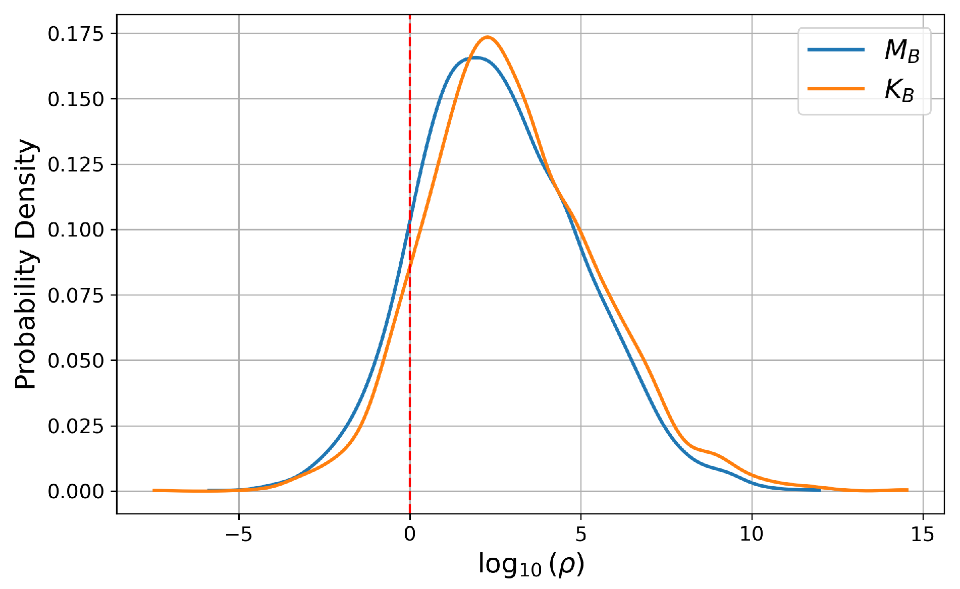
Figure 6 shows the probability density function of ${log}_{10}\left({\rho }_c\right)$ for all classes estimated by using the data in our CSI dataset. As observed in the figure, the distribution is clearly more shifted to the right when our KAN-based classifier is applied than when the MLP-based classifier is used. In particular, compared to the MLP-based classifier, the KAN-based classifier reduces the region where ${log}_{10}\left({\rho }_c\right)<0$, which corresponds to the cases where the model assigns a higher probability to an incorrect class than to the correct one. These results indicate that our KAN-based classifier increases the correct keypad input recognition rate.

Table 3. Sensing accuracy comparison between $M_B$ and $K_B$ for varying $w_o$.

Model	${\mathit{w}}_{\mathit{o}}=0$	${\mathit{w}}_{\mathit{o}}=0.25$	${\mathit{w}}_{\mathit{o}}=0.5$	${\mathit{w}}_{\mathit{o}}=0.75$
$M_B$	74.49%	80.73%	87.68%	96.92%
$K_B$	77.85%	81.11%	90.07%	98.01%

Table 3. Sensing accuracy comparison between $M_B$ and $K_B$ for varying $w_o$.

Model	${\mathit{w}}_{\mathit{o}}=0$	${\mathit{w}}_{\mathit{o}}=0.25$	${\mathit{w}}_{\mathit{o}}=0.5$	${\mathit{w}}_{\mathit{o}}=0.75$
$M_B$	74.49%	80.73%	87.68%	96.92%
$K_B$	77.85%	81.11%	90.07%	98.01%

Figure 5. t-SNE plots for logit vectors produced by $M_B$ and $K_B$ when $w_o=0.5$.

Figure 5. t-SNE plots for logit vectors produced by $M_B$ and $K_B$ when $w_o=0.5$.

Figure 6. Probability distribution function of ${log}_{10}\left({\rho }_c\right)$.

Figure 6. Probability distribution function of ${log}_{10}\left({\rho }_c\right)$.

To further compare the performance between $M_B$ and $K_B$, in

Table 4. Performance comparison between $M_B$ and $K_B$ when $w_o=0.5$.

Method	Accuracy	Precision	Recall	F1 Score	#. Parameters in Classifier
$M_B$	87.68%	87.79%	87.75%	87.71%	150,282
$K_B$	90.07%	90.21%	90.27%	90.18%	57,600

, we compare the precision, recall, F1 score, and the number of parameters used to achieve these performance metrics when $w_o=0.5$. From this table, we can observe that our $K_B$ consistently outperforms the $M_B$ across all metrics. In terms of the sensing accuracy, $M_B$ achieves $87.68\%$, while $K_B$ achieves an accuracy of $90.07\%$, representing a 2.39 percentage point improvement. Furthermore, our $K_B$ achieves the precision, recall, and F1 score values of $90.21\%$, $90.27\%$, and $90.18\%$, respectively, which are higher than those of $M_B$ ($87.79\%$, $87.75\%$, and $87.71\%$, respectively). These results show that since the KAN-based classifier in our keypad input recognition model uses flexible edge-wise functions, it provides superior discriminative power compared to the classifier in $M_B$ that uses a fixed node-wise activation. In addition to the performance improvement, $K_B$ is also highly efficient in terms of the number of parameters used. The number of trainable parameters used to achieve the performance metrics in Table 4 is 150,282 when $M_B$ is used, while it is reduced only to 57,600 when $K_B$ is applied. In other words, we accomplish approximately $62\%$ reduction in the number of trainable parameters.

These results verify that, in contrast to $M_B$, which learns linear relationships with fixed nonlinear activation functions, applying our $K_B$, which learns nonlinear functions to delineate decision boundaries, can enhance the performance of the keypad input sensing and reduce the number of model parameters.

4.3. Impact of Loss Regularization

To investigate the impact of the training loss regularization, we apply $L_{\mathrm{tot}}^{\mathrm{SM}}$ and $L_{\mathrm{tot}}^{\mathrm{CET}}$ not only to $K_B$ but also to $M_B$. Hereafter, we denote $M_B$ trained with $L_{\mathrm{tot}}^{\mathrm{SM}}$ as $M_{SM}$, while $M_B$ trained with $L_{\mathrm{tot}}^{\mathrm{CET}}$ is denoted as $M_{CET}$. We also refer to $K_B$ trained with $L_{\mathrm{tot}}^{\mathrm{SM}}$ as $K_{SM}$, while $K_B$ with $L_{\mathrm{tot}}^{\mathrm{CET}}$ is denoted as $K_{CET}$.

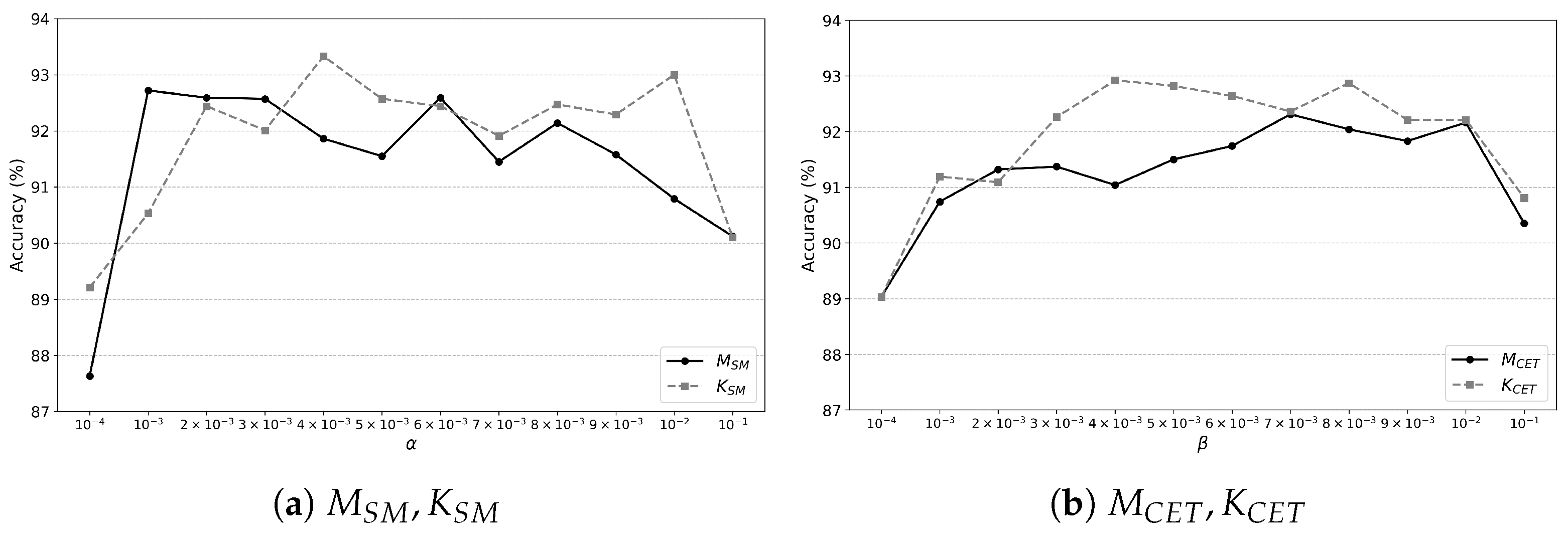
Since the weight $\alpha$ in $L_{\mathrm{tot}}^{\mathrm{SM}}$ and $\beta$ in $L_{\mathrm{tot}}^{\mathrm{CET}}$ affect the sensing accuracy of a model, we investigate the accuracy sensitivity of a model with respect to these parameters. We vary $\alpha$ and $\beta$ from ${10}^{-4}$ to ${10}^{-1}$ and measure the sensing accuracy of each model. Then, we present the results in Figure 7. As illustrated in the figure, when the parameter values are too small or too large, the accuracy of the models decreases substantially. These results are attributed to the influence of these parameters on the total loss. As these parameters approach zero, the effect of loss regularization diminishes. This is equivalent to training each model solely with the cross-entropy loss, which leads to accuracy comparable to that of $M_B$ or $K_B$. In contrast, as the value of these parameters increases, the influence of the regularization term in $L_{\mathrm{tot}}^{\mathrm{SM}}$ and $L_{\mathrm{tot}}^{\mathrm{CET}}$ becomes more significant. Consequently, the model prioritizes minimizing the intra-class distance of feature vectors over classification (i.e., sensing) accuracy, which decreases the sensing performance. In Figure 7, we also observe that when the parameter values are neither too small nor too large, they do not significantly affect the accuracy of the sensing models. Based on these results, when the saliency map-based regularization is used, we set $\alpha =0.001$, while we configure $\beta =0.007$ when the center loss-based regularization is used.

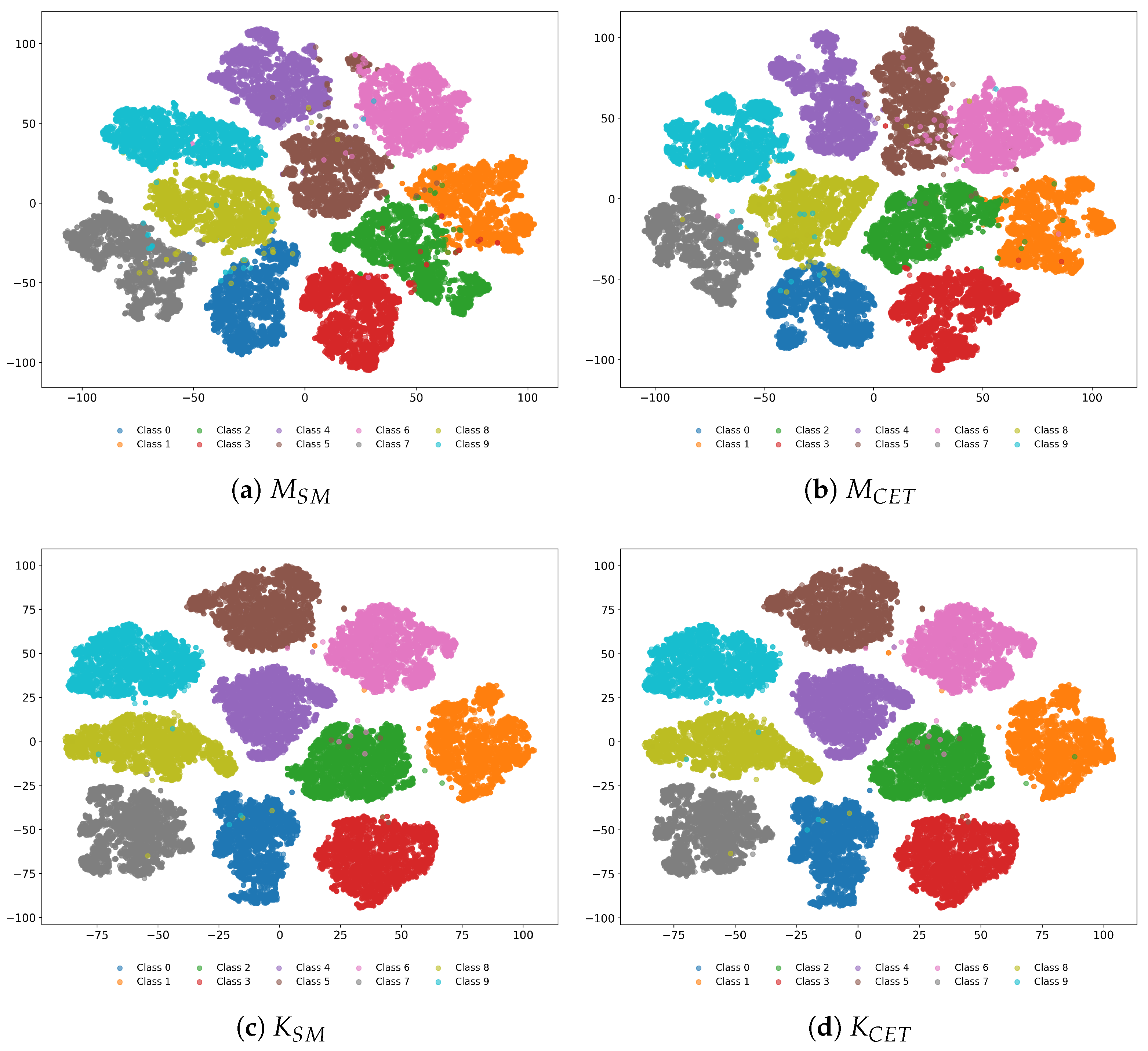
In Figure 8, we illustrate the t-SNE plots for the logit vectors extracted from each model when $w_o=0.5$. Compared to the results in Figure 5, we can see that logit vectors belonging to the same keypad input class are more tightly clustered when the loss regularization is applied than when only the cross-entropy loss is used. These structural differences are closely linked to the improvements in the keypad input recognition accuracy. As shown in the confusion matrices of Figure 9, the models trained with the loss regularization exhibit higher accuracy compared to those without the loss regularization.

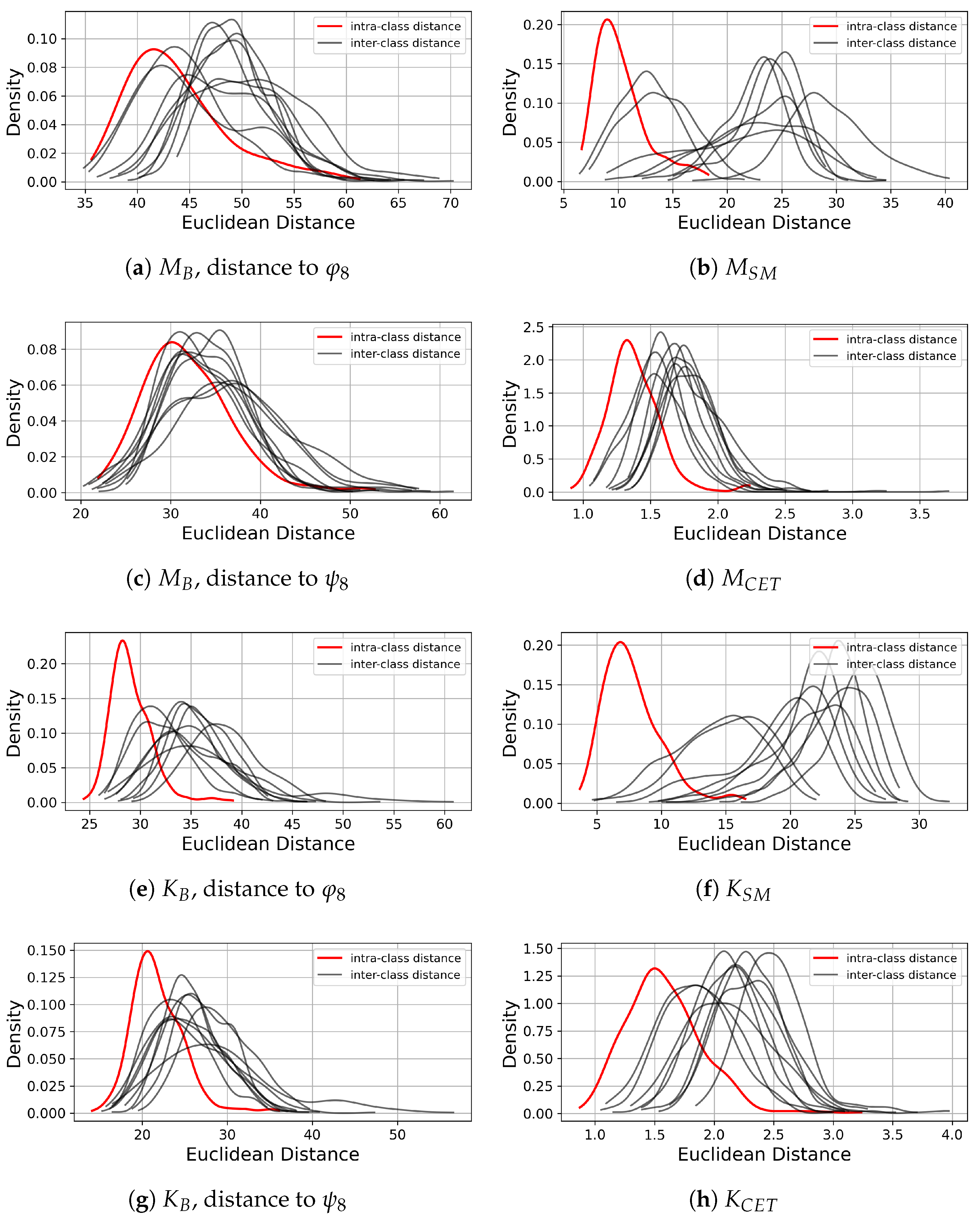
To further analyze the way that the loss regularization affects the class feature structure, in Figure 10, we compare the intra-class distance distribution and the inter-class distance distribution between the feature vectors extracted by a model and the reference point of the class 8 (i.e., ${\phi }_8$ or ${\psi }_8$, depending on the regularization method used). If we denote the set of feature vectors belonging to class i as $W_i$, the intra-class distance represents the Euclidean distance between a feature vector in $W_8$ and the reference point of the class 8. The inter-class distance denotes the Euclidean distance between a feature vector belonging to a keypad input class $i\ne 8$ and the reference point of the class 8. Accordingly, the intra-class distance and the inter-class distance serve as a measure that quantifies the proximity of a feature vector to the reference point. In the case of $M_B$ and $K_B$, to enable comparison with their respective counterparts trained with loss regularization, they are trained using only the cross-entropy loss. Then, the set of feature vectors of the test data are extracted by the trained models. After calculating the reference point of the class 8 among the extracted feature vectors, we compute the distances between the feature vectors of the test data and the reference point of the class 8. In Figure 10, we can observe that when the loss regularization is applied, the distribution of intra-class distances is more concentrated toward smaller values compared to the case without the loss regularization. We can also observe that the use of the loss regularization leads to a rightward shift in the distribution of inter-class distances. These results show that the loss regularization encourages each $Z_f$ to be located close to the corresponding reference point of their class. Correspondingly, the loss regularization increases the intra-class compactness and the structural consistency of the feature space, which contributes to clear separation among classes.

In

Table 5. Comparison of keypad input sensing accuracy among the methods for varying $w_o$.

Model	${\mathit{w}}_{\mathit{o}}=0$	${\mathit{w}}_{\mathit{o}}=0.25$	${\mathit{w}}_{\mathit{o}}=0.5$	${\mathit{w}}_{\mathit{o}}=0.75$
$M_B$	74.49%	80.73%	87.68%	96.92%
$M_{SM}$	80.18%	83.85%	92.72%	98.19%
$M_{CET}$	77.74%	82.40%	92.31%	97.25%
$K_B$	77.85%	81.11%	90.07%	98.01%
$K_{SM}$	80.44%	84.24%	93.33%	98.27%
$K_{CET}$	80.03%	84.08%	92.92%	98.33%

, we compare the sensing accuracy of each model for varying $w_o$. The performance of all the models increases as the amount of CSI data increases. We observe that the loss regularization increases the sensing accuracy regardless of the type of sensing model for all $w_o$. We can also see that the proposed method achieves higher accuracy compared to the CNN models for all $w_o$ and the types of loss regularization. When we compare the saliency map-based regularization and the center loss-based regularization, the former shows higher keypad input recognition accuracy. This is attributed to the way that the reference point is determined. As we can see in Equation (11), ${\phi }_c$ is determined by maximizing the logit value for its corresponding target class while minimizing the average logit value for all non-target classes. In contrast, ${\psi }_c$ is selected based on the Euclidean distance between CSI feature vectors. Consequently, encouraging features of the same class to cluster around ${\phi }_c$, rather than ${\psi }_c$, leads to a higher probability of correct classification. However, as we can see in Table 5, the accuracy difference between the saliency map-based regularization and the center loss-based regularization is not so significant. Thus, the center loss-based regularization is more practical than the saliency map-based regularization in that it can reduce the model training time by half.

Finally, to evaluate the practical applicability of the proposed method in a real computing environment, we evaluate its operational performance on a PC server, which is a common place where the proposed method operates. The server is equipped with an NVIDIA GeForce RTX 4070 SUPER with 12GB RAM, an Intel Core i5-14600KF CPU at 3.50GHz, and 32GB of system RAM. The proposed method is executed using CUDA version 12.7, Python version 3.12.7, and PyTorch version 2.5.1. We separately measure the performance of the CSI preprocessing module and the inference performance of the keypad input recognition module. When we measure the energy consumption, we use CodeCarbon [41]. We present the measurement results in

Table 6. Performance of the proposed method in terms of latency, throughput, and power consumption (NST: number of sensing time).

	Latency (ms)	Throughput (NST/s)	Energy Consumed (kWh)
Preprocessing module	4.99	200.40	9.95 $\times {10}^{-6}$
Recognition module	1.87	534.76	3.69 $\times {10}^{-6}$

, where we observe that the energy consumed during the preprocessing and inference is very low. We can also observe that the proposed method requires more time for CSI preprocessing than for keypad input inference, which limits the sensing throughput of 200.40 times per second. This is attributed to the fact that the CSI preprocessing is primarily handled by the CPU, while the inference is performed by the GPU. However, the total latency remains at 6.86 ms, which is shorter than the CSI measurement interval of 10 ms. In general, the CMD and the PC server are connected via a high-speed network and modern wired and wireless LANs typically support transmission speeds of over 100 Mbps. $x_{i,c}\left(t\right)$ is comprised of an in-phase component and a quadrature component. If we assume that each component is represented by four bytes, the size of a CSI data measured by a CMD becomes $8n_s$ bytes. Since $n_s=52$, the time required to transmit a CSI data from the CMD to the server is 33.28 $\mathsf{\mu }$s, which is negligibly small compared to the 6.86 ms of the total latency. Therefore, we believe that the proposed method is capable of producing sensing results every 10 ms and can be considered suitable for real-time applications.

4.4. Performance Comparison with Other Baselines and in Other Environment

To further evaluate the effectiveness of the proposed method, we compare its performance with those of two other baseline sensing models. The first baseline model is a 1D CNN model in [26] and the second baseline model is based on a ViT (Vision Transformer) [28]. We preserve the original architectures of these models and adjust only their input data formats to accommodate the measured CSI data. In

Table 7. Performance comparison between our model and other baseline models when $w_o=0$.

Method	Accuracy	Precision	Recall	F1 Score
1D CNN	74.80%	75.00%	74.84%	74.76%
ViT	50.66%	50.33%	51.04%	50.99%
$K_B$	77.85%	77.92%	77.94%	77.76%
$K_{SM}$	80.44%	80.98%	80.63%	80.63%
$K_{CET}$	80.03%	81.23%	79.86%	80.12%

and

Table 8. Performance comparison between our model and other baseline models when $w_o=0.5$.

Method	Accuracy	Precision	Recall	F1 Score
1D CNN	87.83%	87.91%	87.96%	87.89%
ViT	59.07%	58.99%	59.42%	58.92%
$K_B$	90.07%	90.21%	90.27%	90.18%
$K_{SM}$	93.33%	93.48%	93.48%	93.40%
$K_{CET}$	92.92%	93.02%	93.02%	93.00%

, we show the results when $w_o$ is 0 and 0.5, respectively. We observe in these tables that the performance of sensing models increases with the amount of training data. In addition, as evidenced by the results in these tables, the proposed approach which combines the KAN-based classifier with the loss regularization demonstrates superior performance compared to the baseline models in terms of the accuracy, precision, recall, and F1 score. We also note that even if the ViT demonstrates strong performance in classifying natural images recognizable by humans, it exhibits limited performance when applied to image representations of CSI data, which is consistent with the results reported in [7].

We also evaluate the performance of our method in a different environment. Specifically, we change the measurement location from a seminar room to the lobby on the first floor of the building. In addition, unlike the previous setting where the keypad is attached to a plastic surface, the keypad is attached to a marble surface in the new environment. The relative positioning among the transmitter, CMD, and keypad is kept consistent with the setup used in the seminar room. To ensure that the CMD can measure CSI every 10 ms, the UDP packet transmission interval of the transmitter is set to 10 ms. Under this configuration, three users each press each keypad button for 4 min, yielding a total of 120 min of collected data. We show the experimental results with this lobby dataset in

Table 9. Comparison among the methods in a lobby environment when $w_o=0.5$.

Model	Accuracy	Precision	Recall	F1 Score
$M_B$	85.54%	86.04%	85.50%	85.57%
1D CNN	85.21%	85.40%	85.20%	85.24%
ViT	51.04%	51.71%	51.26%	50.66%
$K_B$	87.86%	88.03%	87.86%	87.88%
$K_{SM}$	89.57%	89.62%	89.59%	89.56%
$K_{CET}$	89.79%	90.01%	89.73%	89.76%

. As observed in the table, the ViT achieves the lowest performance, whereas the 1D CNN and $M_B$ demonstrate similar levels of performance. The proposed method consistently outperforms the other methods across all the evaluation metrics. In addition, consistent with the results in the seminar room environment, the loss regularization improves the performance of $K_B$ in the lobby environment by encouraging more compact class feature representations.

5. Conclusions and Future Works

In this paper, we propose a novel CSI-based keypad input recognition system called KAN-Sense, which integrates a feature extractor based on convolutional layers with a KAN-based classifier. Using the spline-based nonlinear representations of the KAN, our keypad input recognition model effectively learns complex decision boundaries with significantly fewer parameters compared to a conventional Wi-Fi sensing model based on an MLP-based classifier. To mitigate intra-class variations observed in a keypad input recognition task, we further incorporate two feature regularization methods called a saliency map-based regularization and a center loss-based regularization. Experimental results verify that under equal data conditions, KAN-Sense consistently achieves higher accuracy than the conventional method, regardless of the overall data volume. In addition, in terms of model efficiency, our KAN-based classifier achieves a $62\%$ reduction in the number of trainable parameters relative to the MLP-based classifier when the performance levels of the two methods are set to be comparable. These results demonstrate that the proposed method achieves better classification performance than a conventional method with a MLP-based classifier while requiring fewer parameters. Additionally, we also show that the two regularization methods improve the intra-class compactness and inter-class separability. Consequently, they enhance the sensing accuracy further. These results collectively demonstrate that KAN-Sense enables precise keypad input recognition with low computational complexity and offers strong practical potential for other micro-motion sensing applications.

As our future works, we aim to address the limitations of the current sample-wise data processing approach by designing a model that incorporates temporal context. The current framework processes each CSI sample independently, which prevents the model from capturing the temporal continuity of a single keystroke. To address this limitation, we plan to adopt a sequence-based input representation that aggregates consecutive CSI samples corresponding to a single keystroke for joint processing. Furthermore, we intend to extend this framework to recognize multiple sequential key inputs, thereby enhancing the capability of the system for real-world interactive applications. In addition, we are planning to measure and release CSI data collected from more diverse user populations and sensing environments, aiming to support the development of sensing models with enhanced generalization capabilities. The proposed KAN-Sense system relies on supervised learning, which entails a labeling overhead for CSI data. To overcome this limitation, a key direction for future work is to extend the system to operate under unsupervised learning frameworks.