
Research on Attack Node Localization in Cyber–Physical Systems Based on Residual Analysis and Cooperative Game Theory
Abstract
1. Introduction
- (1)
- Multi-step sampling is introduced within each control period to provide a large amount of effective data for the localization of attacked sensor nodes.
- (2)
- SVM is introduced to perform anomaly detection on the residuals corresponding to each sensor node in the CPS, enhancing the system’s ability to identify anomalies under complex attack scenarios and providing prior information to support the subsequent localization of attacked sensor nodes.
- (3)
- The Shapley value from cooperative game theory is employed to evaluate the contribution of the residuals corresponding to each sensor node to the SVM detection result, providing a decision basis for the localization of attacked sensor nodes.
- (4)
- A voting mechanism is employed within each control period to achieve accurate localization of attacked sensor nodes, addressing the limitations of existing methods in identifying attacked sensor nodes.
2. Related Work
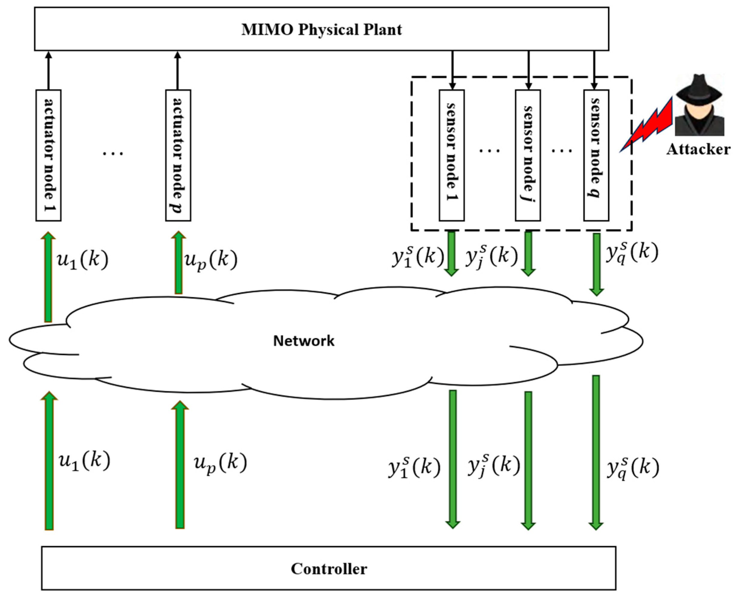
3. System Modeling of CPS and FDI Attack Behavior
3.1. System Modeling of CPS
3.2. FDI Attack Behavior Targeting Sensor Nodes
4. FDI Attack Detection and Attacked Node Localization
4.1. Residual-Based SVM Attack Detection Under Multi-Step Sampling Conditions
4.2. FDI Attack Node Localization Based on Shapley Value and Voting Mechanism
- (1)
- If , it indicates that supports the SVM detection result being anomalous, and thus it is considered as casting a supporting vote for the anomaly detection.
- (2)
- If , it indicates that opposes the SVM detection result being anomalous, and thus it is considered as casting an opposing vote against the anomaly detection.
- (1)
- If
- (2)
- If
- (3)
- If
5. Simulation Results
5.1. SVM Model Training and Detection Performance Evaluation
- (1)
- Accuracy measures the ratio of correctly classified samples to the total number of samples, as shown in Equation (26).
- (2)
- Precision measures the percentage of predicted positive samples that are actually positive, as shown in Equation (27).
- (3)
- Recall indicates the proportion of positive samples that are correctly identified among all actual positive cases, as shown in Equation (28).
- (4)
- The F1 score represents the harmonic average of precision and recall, as shown in Equation (29).
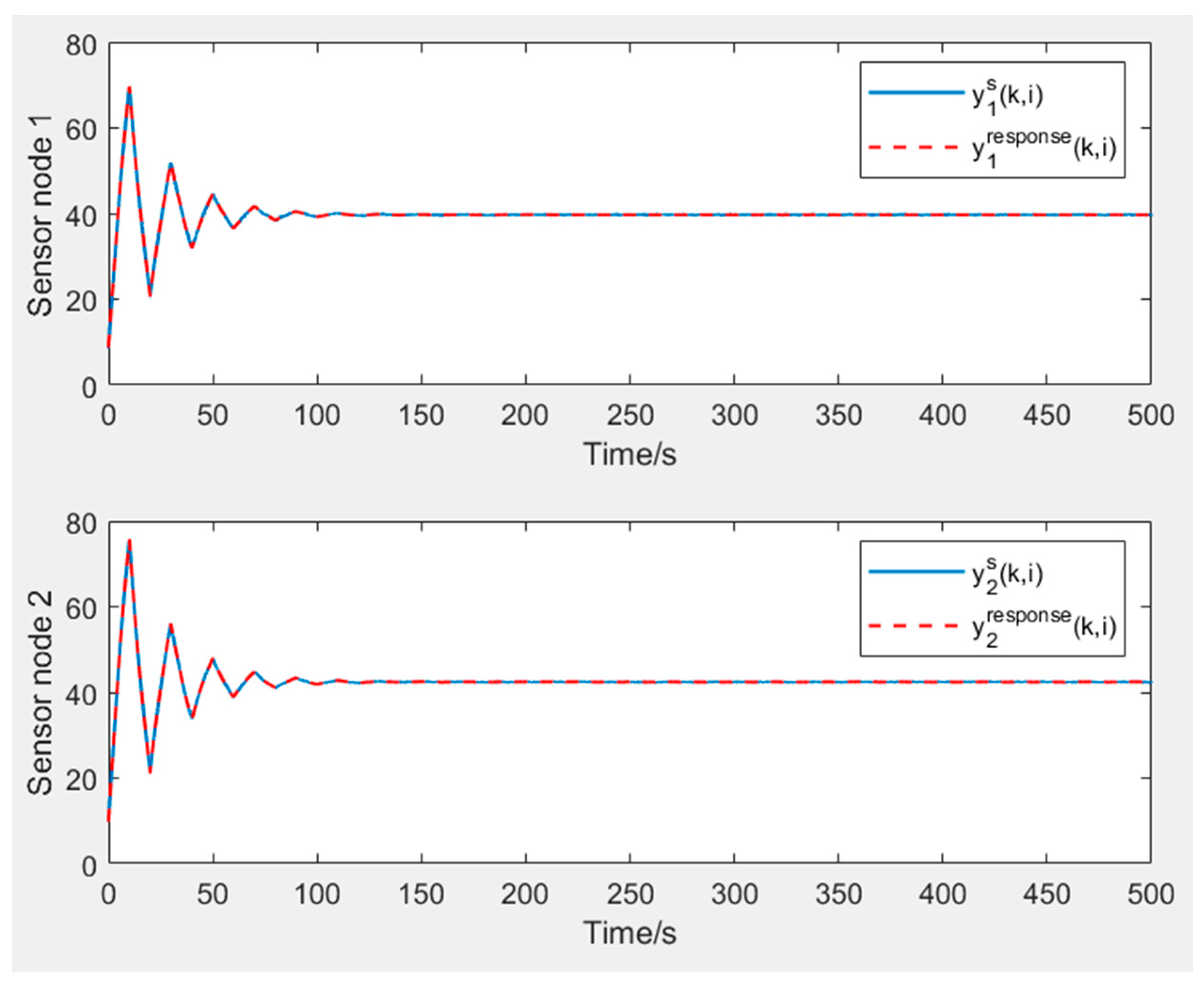
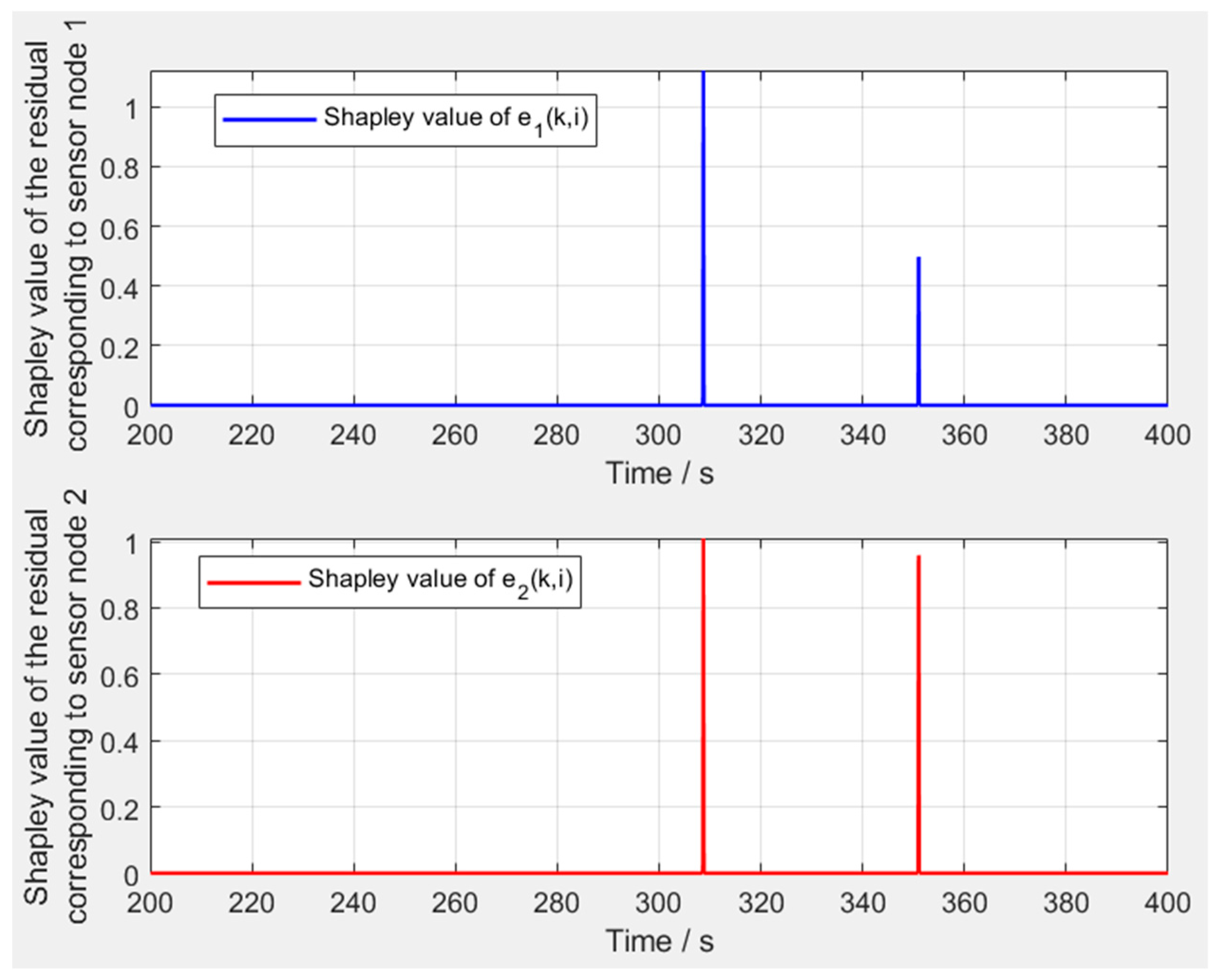
5.2. Voting Analysis and Validation of the Anomalous Node Localization Mechanism
6. Conclusions
Author Contributions
Funding
Data Availability Statement
Conflicts of Interest
References
- Rani, S.; Kataria, A.; Kumar, S.; Karar, V. A new generation cyber-physical system: A comprehensive review from security perspective. Comput. Secur. 2025, 148, 104095. [Google Scholar] [CrossRef]
- Khaitan, S.K.; McCalley, J.D. Design Techniques and Applications of Cyberphysical Systems: A Survey. IEEE Syst. J. 2015, 9, 350–365. [Google Scholar] [CrossRef]
- Yu, Z.; Gao, H.; Cong, X.; Wu, N.; Song, H.H. A survey on cyber–physical systems security. IEEE Internet Things J. 2023, 10, 21670–21686. [Google Scholar] [CrossRef]
- Xu, D.; Tu, M.; Sanford, M.; Thomas, L.; Woodraska, D.; Xu, W. Automated Security Test Generation with Formal Threat Models. IEEE Trans. Dependable Secur. Comput. 2012, 9, 526–540. [Google Scholar] [CrossRef]
- Mo, Y.; Sinopoli, B. Secure control against replay attacks. In 2009 47th Annual Allerton Conference on Communication, Control, and Computing (Allerton); IEEE: Monticello, IL, USA, 2009; pp. 911–918. [Google Scholar] [CrossRef]
- Bayou, L.; Espes, D.; Cuppens-Boulahia, N.; Cuppens, F. Security Issue of WirelessHART Based SCADA Systems. In Risks and Security of Internet and Systems; Lambrinoudakis, C., Gabillon, A., Eds.; CRiSIS 2015; Lecture Notes in Computer Science; Springer: Cham, Switzerland, 2016; Volume 9572. [Google Scholar] [CrossRef]
- Falliere, N.; Liam, O.M.; Chien, E. W32. stuxnet dossier. White Pap. Symantec Corp. Secur. Response 2011, 5, 29. [Google Scholar]
- Case, Defense Use. Analysis of the cyber attack on the Ukrainian power grid. Electr. Inf. Shar. Anal. Cent. 2016, 388, 3. [Google Scholar]
- Rawat, D.B.; Bajracharya, C. Detection of False Data Injection Attacks in Smart Grid Communication Systems. IEEE Signal Process. Lett. 2015, 22, 1652–1656. [Google Scholar] [CrossRef]
- Bi, S.; Zhang, Y.J. Graphical Methods for Defense Against False-Data Injection Attacks on Power System State Estimation. IEEE Trans. Smart Grid 2014, 5, 1216–1227. [Google Scholar] [CrossRef]
- Sedghi, H.; Jonckheere, E. Statistical Structure Learning to Ensure Data Integrity in Smart Grid. IEEE Trans. Smart Grid 2015, 6, 1924–1933. [Google Scholar] [CrossRef]
- Chaojun, G.; Jirutitijaroen, P.; Motani, M. Detecting False Data Injection Attacks in AC State Estimation. IEEE Trans. Smart Grid 2015, 6, 2476–2483. [Google Scholar] [CrossRef]
- Manandhar, K.; Cao, X.; Hu, F.; Liu, Y. Detection of Faults and Attacks Including False Data Injection Attack in Smart Grid Using Kalman Filter. IEEE Trans. Control Netw. Syst. 2014, 1, 370–379. [Google Scholar] [CrossRef]
- Ameli, A.; Hooshyar, A.; Yazdavar, A.H.; El-Saadany, E.F.; Youssef, A. Attack Detection for Load Frequency Control Systems Using Stochastic Unknown Input Estimators. IEEE Trans. Inf. Forensics Secur. 2018, 13, 2575–2590. [Google Scholar] [CrossRef]
- Wang, H.; Ruan, J.; Zhou, B.; Li, C.; Wu, Q.; Raza, M.Q.; Cao, G.-Z. Dynamic Data Injection Attack Detection of Cyber Physical Power Systems With Uncertainties. IEEE Trans. Ind. Inform. 2019, 15, 5505–5518. [Google Scholar] [CrossRef]
- Liu, L.; Esmalifalak, M.; Ding, Q.; Emesih, V.A.; Han, Z. Detecting False Data Injection Attacks on Power Grid by Sparse Optimization. IEEE Trans. Smart Grid 2014, 5, 612–621. [Google Scholar] [CrossRef]
- Wang, Z.; Liu, B.; Chen, J.; Huang, W.; Hu, Y. Nash mixed detection strategy of multi-type network attack based on zero-sum stochastic game. J. Inf. Secur. Appl. 2023, 73, 103436. [Google Scholar] [CrossRef]
- Zhang, J.; Pan, L.; Han, Q.-L.; Chen, C.; Wen, S.; Xiang, Y. Deep learning based attack detection for cyber-physical system cybersecurity: A survey. IEEE/CAA J. Autom. Sin. 2021, 9, 377–391. [Google Scholar] [CrossRef]
- Yan, J.; Tang, B.; He, H. Detection of false data attacks in smart grid with supervised learning. In 2016 International Joint Conference on Neural Networks (IJCNN); IEEE: Vancouver, BC, Canada, 2016; pp. 1395–1402. [Google Scholar] [CrossRef]
- Liu, B.; Chen, J.; Hu, Y. Mode division-based anomaly detection against integrity and availability attacks in industrial cyber-physical systems. Comput. Ind. 2022, 137, 103609. [Google Scholar] [CrossRef]


| Parameter Name | Value |
|---|---|
| Kernel function | RBF |
| Regularization parameter | 10 |
| Kernel width | 0.1 |
| Node 1 Attack Amplitude | 3 or 2 |
| Node 1 Attack Frequency | 0.05 Hz or 0.1 Hz |
| Node 2 Attack Amplitude | 3 or 4 |
| Node 2 Attack Frequency | 0.05 Hz |
| Label Classification | Predicted Label | ||
|---|---|---|---|
| Positive Class (+1) | Negative Class (−1) | ||
| True label | Positive class (+1) | TP | FN |
| Negative class (−1) | FP | TN | |
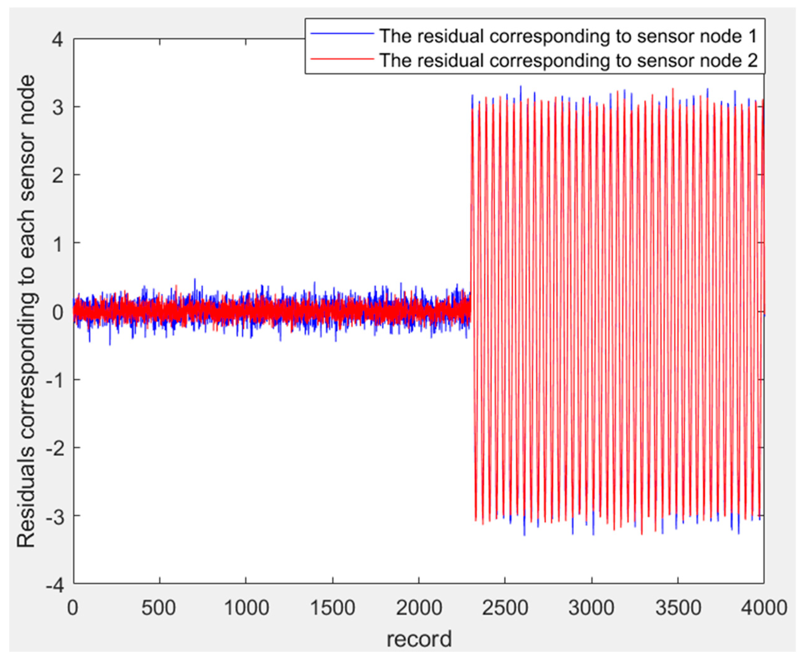
| Item | Description |
|---|---|
| Total samples | 4000 |
| Normal samples | 2300 |
| Anomalous samples | 1700 |
| Feature dimension | 2 (residuals of node 1 and node 2) |
| Sample labels | normal: +1, anomalous: −1 |
| Training set | 1500 normal + 1200 anomalous samples |
| Test set | 800 normal + 500 anomalous samples |
| Accuracy | Precision | Recall | F1 Score |
|---|---|---|---|
| 96.472% | 95.748% | 99.583% | 97.613% |
| Abstentions | Supporting Votes | Opposing Votes | Abstentions | Supporting Votes | Opposing Votes |
|---|---|---|---|---|---|
| 1 | 0 | 0 | 1 | 0 | 0 |
| 1 | 0 | 0 | 1 | 0 | 0 |
| 1 | 0 | 0 | 1 | 0 | 0 |
| 1 | 0 | 0 | 1 | 0 | 0 |
| 1 | 0 | 0 | 1 | 0 | 0 |
| 1 | 0 | 0 | 1 | 0 | 0 |
| 1 | 0 | 0 | 1 | 0 | 0 |
| 1 | 0 | 0 | 1 | 0 | 0 |
| 1 | 0 | 0 | 1 | 0 | 0 |
| 1 | 0 | 0 | 1 | 0 | 0 |
| 0.99 | 0.01 | 0 | 0.99 | 0.01 | 0 |
| 1 | 0 | 0 | 1 | 0 | 0 |
| 1 | 0 | 0 | 1 | 0 | 0 |
| 1 | 0 | 0 | 1 | 0 | 0 |
| 1 | 0 | 0 | 1 | 0 | 0 |
| 0.99 | 0.01 | 0 | 0.99 | 0.01 | 0 |
| 1 | 0 | 0 | 1 | 0 | 0 |
| 1 | 0 | 0 | 1 | 0 | 0 |
| 1 | 0 | 0 | 1 | 0 | 0 |
| 1 | 0 | 0 | 1 | 0 | 0 |
| Abstentions | Supporting Votes | Opposing Votes | Abstentions | Supporting Votes | Opposing Votes |
|---|---|---|---|---|---|
| 0.07 | 0.01 | 0.92 | 0.07 | 0.93 | 0 |
| 0.03 | 0.02 | 0.95 | 0.03 | 0.97 | 0 |
| 0.05 | 0.01 | 0.94 | 0.05 | 0.95 | 0 |
| 0.06 | 0.02 | 0.92 | 0.06 | 0.94 | 0 |
| 0.07 | 0.01 | 0.92 | 0.07 | 0.93 | 0 |
| 0.06 | 0.03 | 0.91 | 0.06 | 0.94 | 0 |
| 0.06 | 0.03 | 0.91 | 0.06 | 0.94 | 0 |
| 0.07 | 0.03 | 0.90 | 0.07 | 0.93 | 0 |
| 0.06 | 0.03 | 0.91 | 0.06 | 0.94 | 0 |
| 0.05 | 0.01 | 0.94 | 0.05 | 0.95 | 0 |
| 0.05 | 0.87 | 0.08 | 0.05 | 0.94 | 0.01 |
| 0.05 | 0.88 | 0.07 | 0.05 | 0.95 | 0 |
| 0.04 | 0.88 | 0.08 | 0.04 | 0.96 | 0 |
| 0.04 | 0.90 | 0.06 | 0.04 | 0.95 | 0.01 |
| 0.03 | 0.88 | 0.09 | 0.03 | 0.97 | 0 |
| 0.04 | 0.90 | 0.06 | 0.04 | 0.96 | 0 |
| 0.05 | 0.87 | 0.08 | 0.05 | 0.95 | 0 |
| 0.05 | 0.90 | 0.05 | 0.05 | 0.95 | 0 |
| 0.04 | 0.91 | 0.05 | 0.04 | 0.96 | 0 |
| 0.05 | 0.87 | 0.08 | 0.05 | 0.95 | 0 |
Disclaimer/Publisher’s Note: The statements, opinions and data contained in all publications are solely those of the individual author(s) and contributor(s) and not of MDPI and/or the editor(s). MDPI and/or the editor(s) disclaim responsibility for any injury to people or property resulting from any ideas, methods, instructions or products referred to in the content. |
© 2025 by the authors. Licensee MDPI, Basel, Switzerland. This article is an open access article distributed under the terms and conditions of the Creative Commons Attribution (CC BY) license (https://creativecommons.org/licenses/by/4.0/).
Share and Cite
Sun, Z.; Jie, X. Research on Attack Node Localization in Cyber–Physical Systems Based on Residual Analysis and Cooperative Game Theory. Electronics 2025, 14, 2943. https://doi.org/10.3390/electronics14152943
Sun Z, Jie X. Research on Attack Node Localization in Cyber–Physical Systems Based on Residual Analysis and Cooperative Game Theory. Electronics. 2025; 14(15):2943. https://doi.org/10.3390/electronics14152943
Chicago/Turabian StyleSun, Zhong, and Xinchun Jie. 2025. "Research on Attack Node Localization in Cyber–Physical Systems Based on Residual Analysis and Cooperative Game Theory" Electronics 14, no. 15: 2943. https://doi.org/10.3390/electronics14152943
APA StyleSun, Z., & Jie, X. (2025). Research on Attack Node Localization in Cyber–Physical Systems Based on Residual Analysis and Cooperative Game Theory. Electronics, 14(15), 2943. https://doi.org/10.3390/electronics14152943