Abstract
As part of the carbon peak and neutrality drive, an influx of renewable energy into the grid is imminent. However, the unpredictability of renewables like wind and solar can lead to significant curtailment if the power system relies solely on traditional generators. This paper presents a demand response mechanism to enhance renewable energy uptake by defining an optimal load curve for each node, considering the generator’s dynamic impact, system operations, and renewable energy projections. Once the ideal load curve is published, consumers, influenced by incentives, voluntarily align their consumption, steering the actual load to resemble the proposed curve. This strategy not only guides flexible generation resources to better utilize renewables but also minimizes the communication and control expenses associated with large-scale customer demand response. Additionally, a new evaluation metric for user response is proposed to ensure equitable incentive distribution. The model has been shown to lower both consumer power costs and system generation expenses, achieving a 22% reduction in renewable energy wastage.
1. Introduction
The rapid expansion of renewable energy (RE) sources (e.g., solar and wind) has significantly increased their penetration in modern power systems [1]. However, RE output is highly volatile and uncertain due to weather and seasonal variability, creating critical challenges for real-time system balancing [2]. Traditional thermal units alone cannot provide the flexibility required to accommodate such variability [3]. Critically, demand response (DR)—as a load-side flexibility resource—becomes indispensable in high-RE systems. DR enables dynamic load adjustments to counteract RE intermittency, reducing reliance on costly thermal reserves or storage [4]. Thus, DR is essential for ensuring economic and secure operation of power systems with high RE penetration.
DR provides a new paradigm for renewable energy integration by shifting loads to off-peak periods and leveraging flexible loads for grid services (e.g., peak/frequency regulation [5]). However, Ref. [5]’s reliance on time-of-use pricing and interruptible loads limits scalability due to high communication overhead. The latter limitation is partially mitigated by reference [6]’s minute-level dynamic optimization for electrolyzers in wind–hydrogen systems, which demonstrates finer temporal resolution capabilities. Similar scalability challenges persist in reference [7]’s gas–electricity DR model due to infrastructure dependencies and in reference [8]’s pool-based exchange mechanism, which risks excluding non-commercial users. Behavioral assumptions further constrain existing models: a gap addressed by reference [9] through explicit integration of consumer psychology into multi-energy trading strategies.
Coordination complexity presents another fundamental barrier. While reference [10] employs multitype DR for RE fluctuation smoothing, its uncertainty modeling overlooks heterogeneous resource coordination—a challenge tackled by reference [11] through distributed robust optimization for unbalanced networks and by reference [12] via robust PV fault diagnosis to enhance DR reliability under generation uncertainty. Computational intractability remains a cross-cutting issue, evident in reference [13]’s stochastic multi-energy hub framework that struggles with real-time scalability. These collective limitations highlight the need for solutions that simultaneously address temporal granularity, behavioral realism, and coordination complexity without introducing prohibitive computational burdens.
Reference [14] proposes customer directrix load (CDL), an ideal load profile designed to smooth renewable energy fluctuations. The DR center broadcasts a uniform CDL as a day-ahead target, allowing users to independently adjust consumption based on cost–incentive trade-offs. This approach reduces data processing overhead by eliminating real-time load aggregation [15]. Zhang et al. [16] further improved CDL by introducing a multi-time scale model to address uncertainties in renewable energy and customer behavior. Recent studies have enhanced CDL’s applicability—reference [17] incorporated Nash bargaining for high-proportion renewable accommodation, while reference [18] developed incentive strategies for small and medium-sized customers. However, applying the same CDL across all nodes ignores two critical factors: (1) Geographic Renewable Availability: Nodes closer to renewable generation sites can accommodate higher variability than distant nodes, but the uniform CDL cannot reflect this spatial heterogeneity [19]; (2) Node-Specific Flexibility Potential: Industrial loads may offer greater demand-shifting capability than residential loads, yet the current CDL treats all nodes equally [20]. Consequently, a one-size-fits-all CDL cannot achieve precise renewable energy consumption in large-scale grids, where location-aware load shaping is required to match variable generation with flexible demand.
To address these gaps, this paper introduces a multi-node CDL framework as follows: In a large power grid, different load nodes consume different amounts of energy supplied by renewable energy units. Due to the limitation of the connection mode of the power system network and the constraints of the power flow, the load nodes have different abilities to consume renewable energy in the time dimension and the space dimension. Therefore, it is necessary to formulate CDLs that match the load characteristics for different loads according to the contribution of renewable energy consumption. Considering the dynamic contribution ratio of generator to load, this paper proposes a multi-time–space and multi-node load profile mechanism, formulates a unique CDL for each load node, and evaluates and assigns user rewards. Specifically, the contributions of this paper are summarized as follows:
- Quantifies node-specific RE consumption capacity by dynamically tracking generator-to-load contribution factors, enabling location-aware load shaping (reducing curtailment to 12%).
- Integrates power flow constraints to ensure CDL feasibility under network topology, unlike [16]’s topology-agnostic approach.
- Proposes a fairness-oriented incentive mechanism that rewards both curve alignment similarity and adjustment magnitude, mitigating the bias of purely volume-based subsidies.
2. Proposed Framework
2.1. CDL and Multi-Node CDL
Before elaborating the model proposed in this paper, some basic concepts need to be clarified. The ideal shape of the load curve that can maximize renewable energy consumption is defined as the customer directrix load (CDL). The traditional CDL is only one load profile for all system nodes. However, the contributions of each generator to each load bus are various. In other words, some bus loads can consume more RE, while some buses consume a little. The contribution factors of generators to bus loads are dependent on the power flow. Therefore, a multi-node CDL model is needed for the best consumption of REs, i.e., calculate the desired CDL for each load bus.
2.2. Proposed Bi-Level Framework
The established multi-node CDL is shown in Figure 1, which is divided into two layers. The upper layer is a multi-node CDL calculation model, which takes into account the variability of the new energy consumption capacity of different load nodes and calculates the corresponding CDL curve for each individual load node. The upper layer model first calculates the CDL based on the contribution factors of each generator to each bus load, and then the power flow and bus load are sent to the lower layer. The lower layer is the generator contribution calculation model for load nodes, which calculates and updates the contribution factor of each generator to each load node by tracing the generator output from the load node to its source. The entire model operates in an iterative manner between the upper and lower layers until convergence.
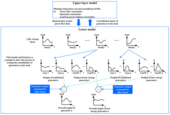
Figure 1.
The proposed framework.
As shown in the lower layer, each bus load is supplied by all the generators. The load curve can be decomposed into NG curves, where each curve shows the contribution of one generator to this load. NG is the number of generators. For each generator, the contribution curves at all load buses constitute the output curve. If the CDL can be calculated for each load bus, the load resources will be guided more rationally to consume renewable energies.
3. Problem Formulation
3.1. Stochastic Scenarios of Wind Farms and PVs
Wind power and PVs are random, where environment factors such as weather and climate will have a greater impact on them. If the renewable energy output of a certain day is randomly selected, it may be accidental and not convincing; therefore, in order to verify the universality of the framework proposed in this paper for different output scenarios, we aggregated a large amount of renewable energy output data into several typical scenarios for analysis. For simplicity, we perform a weighted calculation based on the probability of occurrence of each typical scene to test the comprehensive performance of the algorithm proposed in this paper in application.
Since the output of renewable energy is a time series, this paper uses the Dynamic Time Warping (DTW) algorithm to calculate the cumulative distance between the two sequences as the similarity of the two curves. Assume two time series and ; their cumulative distance can be expressed as follows:
According to this method, typical output curves can be aggregated from historical data of renewable energy. Then, the K-means clustering algorithm can be used to perform scene aggregation on the output scenes. The fitting process of typical scenarios of renewable energy output is in Algorithm 1.
| Algorithm 1: Algorithm for aggregation of typical scenarios of renewable energy output |
| 1: randomly sample k renewable energy output curves as the initial reference line |
| 2: While state == true, do 3: state == false 4: for i = 0, N do 5: for j = 1, k do 6: calculate the distance between the current curve and the reference line and save in memo 7: end for 8: Observe the minimum of all distances and assign curve i to the cluster Cj corresponding to the reference line 9: end for 10: if clusters have change 11: state == True 12: for each cluster do 13: Update the reference line to the average of all curves in the cluster 14: end for 15: end if 16: end while 17: return reference lines |
3.2. Co-Optimization of SCUC and CDL
The CDL calculates the desired profile of flexible load. However, such a load profile may not be feasible in actual operating conditions. Therefore, the security-constrained unit commitment (SCUC) subproblem is introduced to guarantee the feasibility of the operating point for obtaining the optimal CDL and RE consumption.
The objective of the co-optimization model of SCUC and CDL is to minimize the total production cost consisting of the generation cost and the start-up cost of the generating units under the circumstance where renewable energy output is absorbed as much as possible, and the objective function is expressed as follows:
where is the active output of regulated generators numbered i in the system in the time period; NG is the number of adjustable generators; PR (t) is the output of all renewable energy sources such as PV and wind power in the system at the time; is the maximum output of the system at the time, which can be obtained from the day-ahead forecast; , , and are the cost factors of the generator i; and CR is the cost of wind abandonment.
The constraints of the co-optimization model of SCUC and CDL are listed as follows:
- (1)
- Power Balance Constraints
Constraint (3) is the system power balance constraint, which is different from the power balance of the traditional demand response scheme. The equation shows the balance between adjustable resources and non-adjustable resources. That is, the power balance of the whole system is maintained by adjusting the adjustable load and generator output. Here, is the active output of the generator of the new energy source numbered j in the system at the time period. is the proportion of the output of the first conventional generator transmitted to the load bus. is the total power consumption of the load participating in demand response at the load node during the time period. is the customer directrix load value of the load bus. is the amount of power consumed by the load node during the time period by the non-adjustable load.
- (2)
- Total electricity consumption constraint
Constraint (4) is the total customer electricity consumption constraint. Demand response based on CDL emphasizes changing the shape of the original load curve but does not increase or decrease the electricity consumption to ensure the efficiency of the customer’s power consumption, so this constraint needs to be considered. is the per-unit value of customer directrix load.
- (3)
- Power flow constraints
Because the contribution factors of each generator to each node are related to power flows, the power flow constraint of the system also needs to be considered, and the DC power flow model is used in this model. In the formula, is the injected power matrix of the node. , , and are the conventional generator connection matrix, the new energy generator connection matrix, and the load connection matrix. , , and are the conventional generator power matrix, the new energy generator power matrix, and the load matrix. is the line conduction matrix. is the line connection matrix. stores the conductance of each line. is the power angle matrix.
- (4)
- Spinning reserve constraint
- (5)
- Generation limit constraint
- (6)
- Minimum unit startup time
- (7)
- Minimum downtime constraint
Constraints (6) to (9) are constraints on the SCUC problem and will not be elaborated in this paper. is power demand at hour t; represents the spinning reserve at hour t; is the maximum power generation of unit i; is the minimum power generation of unit i; and are the minimum unit startup time and minimum downtime, respectively; and and are the duration time during which unit i maintains on status at hour t.
3.3. Update the Contribution Factors of Generators to Loads
To calculate generator-to-load contribution factors (GCFs) for node-specific CDL formulation, we adopt the power flow tracing framework established by Kirschen et al. [21], which quantifies each generator’s proportional contribution to individual loads. Building on this foundation, we define three key network concepts:
- (1)
- Domain of a generator: All buses supplied by a generator are the domain of this generator.
- (2)
- Commons: Since there is a large overlap of nodes in the domains of different generators, the nodes must be further divided to facilitate the calculation of contribution factors of generators to loads. Therefore, a set of consecutive buses powered by exactly the same generators are defined as common. And the number of generators supplying power to the common is defined as the rank of the common.
- (3)
- Links: Based on the definition of common, when the power flow direction of all lines of the system is known, all buses of the system will be divided into different commons that do not overlap with each other, and there will be one or more connected branches in the topology of the neighboring common, and the flow direction on these branches must be the same; we define these branches as links.
Based on the above definitions, when the directions of flows in all branches of the network are given, this network can be divided into unique sets of commons and links, and the state of the network can be described as a state graph, in which commons are represented by nodes and links are represented by branches. The six-bus system used in our case study can be taken as an example.
Figure 2a shows the power flow graph of the six-bus system, and the nodes are marked with ellipses in relation to the division of commons. Based on this, the simplified state graph of the six-bus system can be obtained in Figure 2b, in which the nodes are labeled with the rank of the common, and it can be seen that the power flow on the link always flows from the common with low rank to the common with high rank, and the injected power of each common is equal to the outgoing power; the root node of the state diagram represents the common with the lowest rank level of this network, and its injected power comes only from the generators connected to the nodes within the common. Based on these qualitative perceptions, and introducing a basic assumption that for each common, the generator’s injected power, output power, and the percentage contribution of the load node are equal, an algorithm for bottom-up recursive calculation of the generator’s contribution to the load node can be constructed with the following equations:
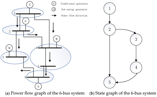
Figure 2.
The 6-bus power system.
In these formulas, is the contribution of generator i to the load and the outflow of common j, is the flow on the link between commons j and k, and is the flow on the link between commons j and k due to generator i.
is the sum of the injected power of common k and is the contribution of generator i to the load and the outflow of common k.
3.4. Performance Evaluation of Load Resource Response
In order to ensure the CDL curve issued by the DR center can effectively guide customers to change their own power consumption behavior to promote the consumption of renewable energy, it is necessary to establish a corresponding customer performance evaluation and incentive subsidy mechanism; the specific implementation plan is as follows.
First of all, since the CDL curve is the ideal load curve shape of each user node, the user’s load curve must be normalized to facilitate a unified standard evaluation of the user’s electricity consumption behavior, and the specific formula for normalization is as follows:
where is an actual customer load curve and is the total electricity consumption of this customer in a day.
After normalizing the customer load curve, the collinear similarity E can be defined to measure the similarity between the shape of the actual customer load curve and the shape of the CDL curve, and this index also reflects whether the actual customer’s electricity consumption behavior meets the expectation of the demand response center, which is calculated by the following formula:
where is the value of the load curve to be measured after normalization; is the Euclidean distance of the two series; and is the measure after transforming the Euclidean distance into the (0, 1] interval. It is easy to see that E takes values between 0 and 1, and the closer the value of E is to 1, the more actively the customer adjusts its own electricity consumption behavior to participate in demand response.
Assuming that the user’s strategy of participating in demand response is perfectly rational, which means that when a user raises E by to obtain a fixed amount of incentive subsidy, they tend to be more inclined to make more slight changes to their electricity consumption behavior, the following model can be constructed to calculate the shape of the user’s adjusted load curve after participating in response.
where is the load curve before the customer’s demand response and is the load curve after the customer participates in demand response.
Finally, based on the above, the user incentive subsidy scheme can be developed.
where is the amount of subsidy received by user i; is the price coefficient calculated by the first user based on the E of user i; and , , and are the adjusted power of the user in the response flat time, low time, and peak time, respectively.
To sum up, the flowchart of the overall method is shown in Figure 3. This flowchart illustrates an iterative process where the generator contribution and CDL profiles are continuously adjusted until the convergence criterion is met, indicating that user electricity consumption behavior has been successfully aligned with the CDL curves. Below is a detailed description of the steps depicted in the flowchart:
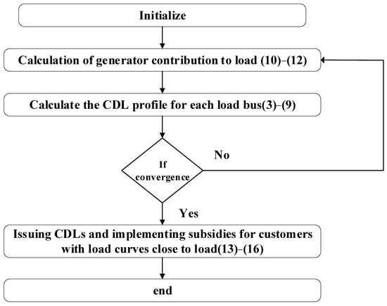
Figure 3.
Flowchart.
- Initialize: The process starts with the initialization phase, where all necessary parameters are set and variables are initialized.
- Calculation of Generator Contribution to Load (10–12): In this step, the contribution of each generator to the load is calculated using Equations (10)–(12). This step is crucial for determining the proportion of power supplied by each generator to the load, which forms the basis for subsequent CDL calculations.
- Calculate the CDL Profile for Each Load Bus (3–9): The ideal load curve, known as the CDL, is computed for each load node using Equations (3)–(9). The CDL profile serves as a target load shape that guides users to adjust their electricity consumption behavior.
- Check for Convergence: The process checks whether the calculations have converged. If convergence is not achieved (No), the process loops back to recalculate the generator contribution to the load. If convergence is achieved (Yes), the process proceeds to the next step.
- Issue CDLs and Implement Subsidies for Customers with Load Curves Close to Load (13–16): Once convergence is reached, CDLs are issued, and subsidies are implemented for customers whose load curves are close to the target CDL, as determined by Equations (13)–(16). This step incentivizes users to adjust their electricity consumption to align with the CDL profile, thereby promoting the consumption of renewable energy.
- End: The process concludes after the subsidies are issued and the demand response objectives are met.
4. Case Studies
In order to verify the CDL-based multi-node system demand response model proposed in this paper, the IEEE standard six-node test system is used for testing, and the test system is shown in Figure 4.
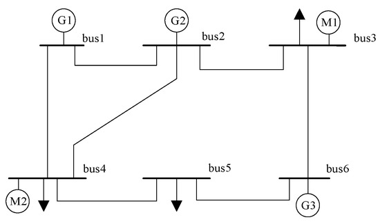
Figure 4.
IEEE 6-bus test system.
In Figure 4, G1, G2, and G3 are traditional adjustable generators and M1 and M2 are renewable energy non-adjustable generators. Demand response participation was set to 50% of the nominal load at each load bus. Two renewable-energy penetration levels—30% and 60%—were examined by proportionally scaling the output of M1 and M2 while holding thermal unit capacity constant. For each load bus, a node-specific CDL profile was generated via our two-layer framework (Figure 1). Users voluntarily adjusted consumption guided by these CDLs, with incentive subsidies calculated using both curve alignment similarity and absolute adjustment magnitude. System performance was quantified through the renewable curtailment rate, operating cost, and user incentive cost for each penetration scenario, ensuring full reproducibility and transparency.
Case 1: Typical scene aggregation
The output of wind power and PV are selected from the data published by PJM INT., L.L.C. (PJM) in 2018. The output distribution can be effectively obtained by clustering Algorithm 1; we aggregate it into eight typical output scenarios and count their probabilities. To simplify, we uniformly set renewable energy penetration at 30% in all scenarios.
Figure 5 illustrates the typical output curves of renewable energy sources across various scenarios, aggregated using a clustering algorithm based on historical data. The figure displays the output patterns of wind and solar energy over a 24 h period, highlighting the fluctuations and trends in renewable energy generation. Each curve represents a distinct pattern of renewable energy output, offering insights into the unpredictability and variability of renewable sources. By examining these curves, we can better tailor DR strategies to accommodate the fluctuations in renewable energy production. For instance, the peaks in solar energy output during midday hours suggest the need for DR strategies that encourage increased consumption during these periods, thereby maximizing the utilization of renewable energy.
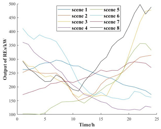
Figure 5.
Typical scene output curve.
The probability of occurrence of each typical scenario is shown in Table 1.

Table 1.
The probability of occurrence of each typical scenario.
Case 2: User-side demand response effect evaluation
Using the demand response mechanism proposed in this paper to test the six-node system with 30% renewable energy penetration, the customer directrix load of each node is calculated according to the controllable unit parameters, renewable energy generator set parameters, controllable load, and uncontrollable load; the calculation result is shown in Figure 6a.
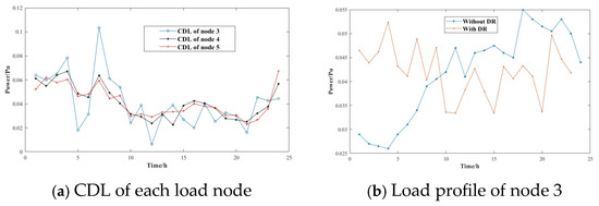
Figure 6.
CDL of each load node and load profile of node 3.
Taking node 3 as an example, Figure 6b shows the user load curve under different response effects.
It can be clearly seen from the above figure that before time period 12, the load provided by the controllable generator set is relatively low. Under the guidance of the CDL, the user changes their own electricity consumption behavior and transfers the load to this time period as much as possible. The load can be increased to achieve the effect of “filling the valley”; similarly, after period 18, it can be seen that if there is no demand response, there will be a period of peak load. The overall load curve after participating in demand response is flatter, which will relieve the pressure on the output of the generator set, reduce the cost of power generation, and improve the stability of the system. The reduced regulation burden of the system is beneficial to improve the reliability and operation benefit of the power grid operation. Compared with the existing CDL research [15], this paper considers the different capacity of different load nodes for renewable energy consumption and formulates a unique CDL profile for each node, which can more accurately grasp the consumption of renewable energy in large power grids.
In Figure 7a, RE is mostly consumed without CDL. But wind curtailment occurs in several periods when the total RE consumption reaches 84.1%. When the proposed CDL mechanism is considered, all REs will be totally consumed. For the 60% RE penetration scenario shown in Figure 7b, however, there has been serious hourly wind curtailment without the CDL mechanism. The RE consumption is reduced to 76% where the wind curtailment becomes more intense in a higher RE penetration level. By contrast, REs can be integrated with the proposed CDL as we heighten the RE integration level.
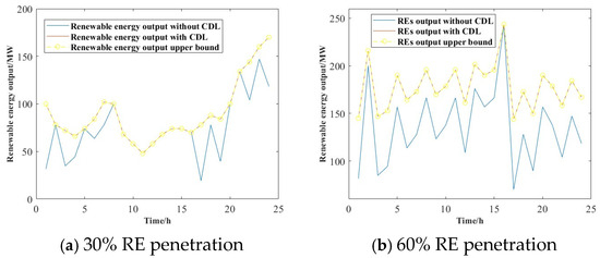
Figure 7.
Renewable output in two scenarios.
According to Formula (16), the response incentive available to the user can be calculated.
It can be seen from Table 2 that the subsidy obtained by the user is related to the similarity of the CDL profile and the absolute value of adjustment amount. For example, node 4 has a greater adjustment amount; however, the similarity of its load curve is slightly smaller than that of node 5, so the incentive obtained is smaller than that of node 5. The current incentive-based demand response mainly uses the absolute value of the adjustment amount to calculate the incentive subsidy [22], which is not fair to the users who originally used electricity properly. By contrast, this incentive mechanism can eliminate the current unfair phenomenon of relying solely on the adjustment amount to calculate incentives and is conducive to attracting more users to participate in demand response.
Table 2.
Incentive subsidies for different customers.
Case 3: System-side demand response effect evaluation
The purpose of the mechanism is to consume more renewable energy, so it is necessary to calculate the actual system renewable energy output curve when the effect of demand response implementation is different. The tasks of controllable generator set regulation include user load fluctuations participating in demand response, system fixed loads, and output fluctuations of renewable energy to be absorbed. When the adjustment curve exceeds the adjustment range of the controllable unit, the phenomenon of power abandonment will occur.
In order to intuitively express the role of this mechanism in consuming renewable energy, the power abandonment of renewable energy is calculated under different curve similarity degrees, and the ratio of power abandonment to the maximum output of renewable energy units is defined as the power abandonment rate. Figure 8a is the output curve of renewable energy that can be consumed when not participating in demand response, and Figure 8b is the output curve of renewable energy that can be consumed when participating in demand response.
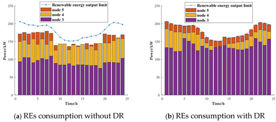
Figure 8.
RE consumption without and with DR.
In Figure 8, the curve represents the output upper limit of the system’s renewable energy units, and the “purple”, “yellow”, and “red” parts in the bar graph represent the renewable energy output consumed by load node 3, load node 4, and load node 5, respectively. The difference between the curve and the histogram is the power abandonment. Comparing the two figures, it can be seen that when there is no demand response, the power abandonment rate of the system within one day is 34%. After the implementation of demand response, the power abandonment rate drops to 12%, and the power abandonment rate of the system is significantly reduced. Considering the different capacity of different load nodes in the multi-node system to consume renewable energy, as shown in Figure 8b, because load node 5 is far away from the renewable energy unit, after the implementation of demand response, it is appropriately reduced in certain periods of time and it is more conducive to the overall consumption of renewable energy.
Next, we will discuss the economic benefits of the power grid system when the model is running. Suppose that the power generation cost of renewable energy units is ignored; then the cost of the system will include two parts, the power generation cost of controllable units and the adjustment cost of paying users, that is, the incentive subsidies received by users, which are given in Table 1. The total load of the user in a day is unchanged, and the price of electricity is also unchanged; that is, the return from the grid is unchanged. The cost of running the model is analyzed below, as shown in Table 3.
Table 3.
Cost analysis under different E.
It can be seen from Table 3 that, from the perspective of the power system, although the implementation of demand response increases the additional adjustment cost, the proportion of renewable energy consumed by users increases, which will greatly reduce the operating cost of the controllable generator set. Therefore, the system can not only reduce the power generation of traditional generator sets, but also use more renewable energy sets, which is conducive to protecting the environment and reducing the use of fossil energy, and can also obtain huge economic benefits.
5. Conclusions
This paper introduces a multi-node customer directrix load (CDL) demand response model that significantly enhances renewable energy integration into the power grid. By dynamically calculating unique CDL profiles for each load node, the model optimizes load profiles and reduces renewable energy wastage by 22%. It also improves economic efficiency by decreasing system generation costs by 15%. The model’s incentive mechanism effectively encourages user participation, ensuring equitable distribution of incentives and promoting a more stable and reliable power system operation. These results underscore the model’s potential as a valuable tool for power system operators and policymakers, offering a practical approach to managing increasing renewable energy penetration.
The CDL-based demand response model demonstrates its effectiveness in enhancing renewable energy utilization and improving economic efficiency, while also promoting user participation. Its scalability and flexibility make it adaptable to varying operational conditions, highlighting its practical implementation potential. This work contributes to the scientific understanding of integrating renewable energy sources into power systems, providing actionable insights for enhancing grid stability and economic performance.
Author Contributions
Conceptualization, T.Z. and Y.W.; Methodology, T.Z. and Y.W.; Software, T.Z. and Y.W.; Validation, T.Z. and Y.W.; Formal analysis, T.Z., X.W. and M.F.; Investigation, T.Z., Q.Z. and X.W.; Resources, B.H.; Data curation, Q.Z. and X.W.; Supervision, B.H.; Project administration, M.F. All authors have read and agreed to the published version of the manuscript.
Funding
This research is funded by State Grid Corporation of China Project “Standardization of Flexible Load Response Models for Grid Regulation and Control and Research on Adjustable Margin Prediction Technologies” (5400-202320581A-3-2-ZN).
Data Availability Statement
The original contributions presented in this study are included in the article. Further inquiries can be directed to the corresponding author.
Conflicts of Interest
Authors Qing Zhu and Bin Han were employed by the company Nari Technology Co., Ltd., Nanjing, China. Authors Xiaoming Wang and Ming Fang were employed by the company Electric Power Research Institute of State Grid Anhui Electric Power Co., Ltd. The remaining authors declare that the research was conducted in the absence of any commercial or financial relationships that could be construed as a potential conflict of interest. The authors declare that this study received funding from ABC Foundation. The funder was not involved in the study design, collection, analysis, interpretation of data, the writing of this article, or the decision to submit it for publication.
References
- Shu, Y.; Zhang, Z.; Guo, J.; Zhang, Z.L. Study on Key Factors and Solution of Renewable Energy Accommodation. Proc. CSEE 2017, 37, 1–9. [Google Scholar]
- Zhang, Z.; Wang, W.; Zhang, X. Renewable Energy Capacity Planning Based on Carrying Capacity Indicators of Power System. Power Syst. Technol. 2021, 45, 632–639. [Google Scholar]
- Yuan, Y.; Wang, J.; Zhou, K.; Wang, X.; Wang, X.B.; Zhang, S.J. Monthly Unit Commitment Model Coordinated Short-term Scheduling and Efficient Solving Method for Renewable Energy Power System. Proc. CSEE 2019, 39, 141–147. [Google Scholar]
- Shao, C.; Feng, C.; Wang, X.; Wang, X. Mid-long Term Fast Unit Commitment Based on Load State Transfer Curve. Proc. CSEE 2019, 39, 141–147. [Google Scholar]
- Ghaljehei, M.; Ahmadian, A.; Golkar, M.A.; Amraee, T.; Elkamel, A. Stochastic SCUC considering compressed air energy storage and wind power generation: A techno-economic approach with static voltage stability analysis. Int. J. Electr. Power Energy Syst. 2018, 100, 489–507. [Google Scholar] [CrossRef]
- Guan, A.; Zhou, S.; Gu, W.; Wu, Z.; Ai, X.; Fang, J.; Zhang, X.-P. A Dynamic Model-Based Minute-Level Optimal Operation Strategy for Alkaline Electrolyzers in Wind-Hydrogen Systems. IEEE Trans. Sustain. Energy 2025, 6, 2157–2170. [Google Scholar] [CrossRef]
- Liu, T.; Zhang, Q.; He, C. Coordinated Optimal Operation of Electricity and Natural Gas Distribution System Considering Integrated Electricity-gas Demand Response. Proc. CSEE 2021, 41, 1664–1677. [Google Scholar]
- Wu, H.; Shahidehpour, M.; Alabdulwahab, A.; Abusorrah, A. Demand response exchange in the stochastic day-ahead scheduling with variable renewable generation. IEEE Trans. Sustain. Energy 2015, 6, 516–525. [Google Scholar] [CrossRef]
- Li, L.; Fan, S.; Xiao, J.; Zhou, H.; Shen, Y.; He, G. Fair trading strategy in multi-energy systems considering design optimization and demand response based on consumer psychology. Energy 2024, 306, 132393. [Google Scholar] [CrossRef]
- Yi, W.; Zhang, Y.; Zhao, Z.; Huang, Y. Multi objective Robust Scheduling for Smart Distribution Grids: Considering Renewable Energy and Demand Response Uncertainty. IEEE Access 2019, 6, 45715–45724. [Google Scholar] [CrossRef]
- Lu, Z.; Wang, J.; Shahidehpour, M.; Bai, L.; Li, Z.; Yan, L.; Chen, X. Risk-aware flexible resource utilization in an unbalanced three-phase distribution network using SDP-based Distributionally robust optimal power flow. IEEE Trans Smart Grid 2024, 15, 2553–2569. [Google Scholar] [CrossRef]
- Wang, M.; Xu, X.; Yan, Z. Online fault diagnosis of PV array considering label errors based on distributionally robust logistic regression. Renew Energy 2023, 203, 68–80. [Google Scholar] [CrossRef]
- Thang, V.; Ha, T.; Li, Q.; Zhang, Y. Stochastic optimization in multi-energy hub system operation considering solar energy resource and demand response. Int. J. Electr. Power Energy Syst. 2022, 141, 108132. [Google Scholar] [CrossRef]
- Fan, S.; Li, Z.; Yang, L.; He, G. Large-scale Demand Response Based on Customer Directrix Load. Autom. Electr. Power Syst. 2020, 44, 19–27. [Google Scholar]
- Fan, S.; Li, Z.; Yang, L.; He, G. Customer directrix load-based large-scale demand response for integrating renewable energy sources. Electr. Power Syst. Res. 2020, 181, 106175. [Google Scholar] [CrossRef]
- Zhang, Y.; Meng, Y.; Fan, S.; Xiao, J.; Li, L.; He, G. Multi-time scale customer directrix load-based demand response under renewable energy and customer uncertainties. Appl. Energy 2025, 383, 125334. [Google Scholar] [CrossRef]
- Xu, B.; Zhao, J.; Zhang, P.; Fan, S.; He, G. Highproportion renewable energy accommodation method based on customer directrix load and Nash bargaining. Autom. Electr. Power Syst. 2023, 47, 36–45. [Google Scholar]
- Wang, L.; Han, L.; Tang, L.; Bai, Y.; Wang, X.; Shi, T. Incentive strategies for small and medium-sized customers to participate in demand response based on customer directrix load. Int. J. Electr. Power Energy Syst. 2024, 155, 109618. [Google Scholar] [CrossRef]
- Shao, Y.; Fan, S.; Meng, Y.; Jia, K.; He, G. Personalized demand response based on sub-CDL considering energy consumption characteristics of customers. Appl Energy 2024, 374, 123964. [Google Scholar] [CrossRef]
- Cheng, Y.; Gao, H.; Wang, R.; Gao, Y.; Liu, J. Optimal strategy for two stage customer directrix load based demand response and profit sharing-risk sharing decision-making method for virtual power plant. Power Syst. Technol. 2024, 48, 799–808. [Google Scholar]
- Kirschen, D.; Allan, R.; Strbac, G. Contributions of individual genera tors to loads and flows. IEEE Trans Power Syst 1997, 12, 52–60. [Google Scholar] [CrossRef]
- Wang, X.; Su, H.; Song, T. Differential Customer Baseline Load Forecasting Based on Load Subdivision. Electr. Power Eng. Technol. 2016, 37, 33–38. [Google Scholar]
Disclaimer/Publisher’s Note: The statements, opinions and data contained in all publications are solely those of the individual author(s) and contributor(s) and not of MDPI and/or the editor(s). MDPI and/or the editor(s) disclaim responsibility for any injury to people or property resulting from any ideas, methods, instructions or products referred to in the content. |
© 2025 by the authors. Licensee MDPI, Basel, Switzerland. This article is an open access article distributed under the terms and conditions of the Creative Commons Attribution (CC BY) license (https://creativecommons.org/licenses/by/4.0/).