Life-Threatening Ventricular Arrhythmia Identification Based on Multiple Complex Networks

Abstract

Ventricular arrhythmias (VAs) are critical cardiovascular diseases that require rapid and accurate detection. Conventional approaches relying on multi-lead ECG or deep learning models have limitations in computational cost, interpretability, and real-time applicability on wearable devices. To address these issues, a lightweight and interpretable framework based on multiple complex networks was proposed for the detection of life-threatening VAs using short-term single-lead ECG signals. The input signals were decomposed using the fixed-frequency-range empirical wavelet transform, and sub-bands were subsequently analyzed through multiscale visibility graphs, recurrence networks, cross-recurrence networks, and joint recurrence networks. Eight topological features were extracted and input into an XGBoost classifier for VA identification. Ten-fold cross-validation results on the MIT-BIH VFDB and CUDB databases demonstrated that the proposed method achieved a sensitivity of 99.02 ± 0.53%, a specificity of 98.44 ± 0.43%, and an accuracy of 98.73 ± 0.02% for 10 s ECG segments. The model also maintained robust performance on shorter segments, with 97.23 ± 0.76% sensitivity, 98.85 ± 0.95% specificity, and 96.62 ± 0.02% accuracy on 2 s segments. The results outperformed existing feature-based and deep learning approaches while preserving model interpretability. Furthermore, the proposed method supports mobile deployment, facilitating real-time use in wearable healthcare applications.

1. Introduction

Sudden Cardiac Death (SCD) is a major public health issue, causing around 300,000 deaths annually in the United States [1]. It is frequently triggered by malignant ventricular arrhythmias, including ventricular fibrillation (VF), ventricular flutter (VFL), and pulseless ventricular tachycardia (VT) [2]. Shockable ventricular arrhythmias (SVAs) involve rapid, irregular ventricular electrical activity, which, if untreated, can lead to death within minutes [3]. Timely detection and accurate categorization of shockable and non-shockable rhythms (NSRs) are therefore essential for initiating life-saving interventions like defibrillation [4].

Recent advances in electronic technology—particularly in low-power microprocessors, flexible sensors, and wireless modules—have accelerated the application of wearable devices for continuous vital sign monitoring [5,6]. Miniaturized ECG front-end chips and photoplethysmography sensors now enable high-precision, high-sampling-rate data collection in compact devices [7,8]. Simultaneously, edge computing platforms like ARM Cortex-M series MCUs and AI inference accelerators support real-time signal processing and basic diagnostic tasks [9], making large-scale, continuous monitoring feasible [10].

Among acute cardiovascular events, ventricular arrhythmias (VAs) remain highly lethal due to their sudden onset and short duration [11]. VAs include premature ventricular contractions, sustained VT, and VF [12]. Compared with Holter monitors or implantable defibrillators, wearable devices offer a more comfortable, portable, and noninvasive alternative for long-term monitoring [13]. However, this also imposes stricter demands on device reliability, power efficiency, and stable operation under diverse conditions [14].

Despite improvements in signal quality using multi-lead arrays, nano-coated electrodes, and hardware filtering [9], baseline drift and motion artifacts persist due to sweat, impedance changes, and ambient interference [15,16]. These distortions impair feature extraction and classification accuracy, making efficient multi-stage filtering and artifact suppression on resource-limited devices a persistent challenge.

Conventional VA detection methods relying on QRS onset or T-wave localization require high computational and memory overhead, rendering millisecond-level real-time detection impractical on embedded platforms [6]. Additionally, waveform distortions increase false-positive and false-negative risks [7]. This highlights the need for lightweight, hardware-friendly algorithms that minimize reliance on multi-lead setups and precise feature localization while ensuring fast, reliable arrhythmia detection in wearable applications.

Earlier studies employed manual feature extraction, rule-based algorithms, and machine learning techniques. Martis et al. applied principal component, linear discriminant, and independent component analyses for ECG beat classification [17]. Sabut et al. combined signal processing with deep learning to enhance VA detection [18]. Although effective, these methods are sensitive to noise and require expert-defined features [19], while machine learning models like SVMs and decision trees still depend on preprocessing and feature selection [20].

Deep learning, especially convolutional and recurrent neural networks, offers improved accuracy by automating feature extraction. Acharya et al. showed that CNNs could effectively detect arrhythmias from ECG segments [21], while Oh et al. integrated CNNs with LSTMs for arrhythmia classification across various ECG lengths [22]. These models reduce the need for manual feature engineering [23], though they require large labeled datasets and substantial computational resources and lack interpretability [24].

To address these issues, complex network analysis has gained interest. By representing ECG signals as networks, it enables the analysis of temporal and spatial dynamics through graph-theoretic measures [25]. Metrics such as degree distribution, clustering coefficient, and shortest path length reflect signal complexity and structure, aiding arrhythmia classification [26]. Garcia et al. demonstrated high accuracy using network features for arrhythmia classification [27], while Liu et al. used network centrality measures to distinguish VF and VT from non-shockable rhythms [28]. Moreover, complex network analysis can be integrated with machine learning and deep learning techniques to enhance both interpretability and classification performance [29]. However, most existing methods focus solely on either single-frequency-band analysis or a single network model, which neglect important dynamic and cross-frequency interactions within ECG signals. To address these limitations, a multi-band, multi-network framework combining lightweight signal decomposition and interpretable network-based features is presented [30] to balance detection performance with computational efficiency for mobile health applications.

In summary, while traditional and deep learning methods have improved arrhythmia detection, limitations in noise sensitivity, computational cost, and model transparency persist. Complex network analysis offers a promising, interpretable alternative for arrhythmia detection, especially when integrated with machine learning and deep learning techniques. In this study, a novel detection framework is proposed that integrates multiple types of complex network models, including visibility graphs, recurrence networks, cross-recurrence networks, and joint recurrence networks. These models can comprehensively characterize the dynamic, nonlinear properties of ECG signals across multiple frequency bands. Unlike most existing approaches that rely on handcrafted features or end-to-end deep learning architectures with limited transparency, this method extracts interpretable network-based topological features, capturing both temporal recurrence and inter-frequency interactions. The extracted features are combined using an XGBoost classifier, which provides a balance between accuracy, interpretability, and computational efficiency. The proposed method addresses existing challenges such as noise sensitivity, dependency on R-wave detection, and deep model opacity. In the future, it can advance the field toward more reliable and clinically applicable solutions for arrhythmia detection.

2. Materials and Methods

2.1. Database and Preprocessing

2.1.1. Benchmark Datasets

Two open-source datasets containing multimodal physiological signals were used, namely the MIT-BIH Malignant Ventricular Ectopy Database (VFDB) dataset and the CU Ventricular Tachyarrhythmia Database (CUDB) dataset.

VFDB: The VFDB is a comprehensive ECG resource consisting of 22 dual-lead ECG recordings, each approximately 35 min in duration. These recordings were taken from patients who experienced severe cardiac events such as sustained ventricular tachycardia, ventricular flutter, and ventricular fibrillation. The data were captured at a sampling rate of 250 Hz, ensuring high-quality signal resolution for detailed analysis. This database is carefully annotated with a wide range of cardiac rhythm abnormalities. These annotations include atrial fibrillation, asystole, ventricular bigeminy, heart block, ventricular ectopy, junctional rhythm, normal sinus rhythm, sinus bradycardia, supraventricular tachycardia, ventricular escape beats, ventricular fibrillation, ventricular flutter, and ventricular tachycardia. To avoid redundancy, only the first-lead ECG data was used in this study.

CUDB: The CUDB was collected by Floyd M. Nolle at the Cardiac Center of Creighton University. It consists of 35 single-lead ECG recordings, each approximately 8 min in length, from patients who experienced severe cardiac events such as sustained ventricular tachycardia, ventricular flutter, and ventricular fibrillation. The ECG signals were sampled at a frequency of 250 Hz, providing high-resolution data. The recordings include 127,232 samples per record. The recording labeled cu01 was obtained from a long-term ECG recording, while the other recordings were acquired from real-time signals from patient monitors. In this database, all detected heartbeats are labeled as normal, and the VF rhythms are marked with the approximate onset of VF episodes. The average time from the beginning of the ECG recording to the onset of VF is 5 min and 47 s. Notably, five records (cu12, cu15, cu24, cu25, and cu32) were obtained from patients with pacemakers.

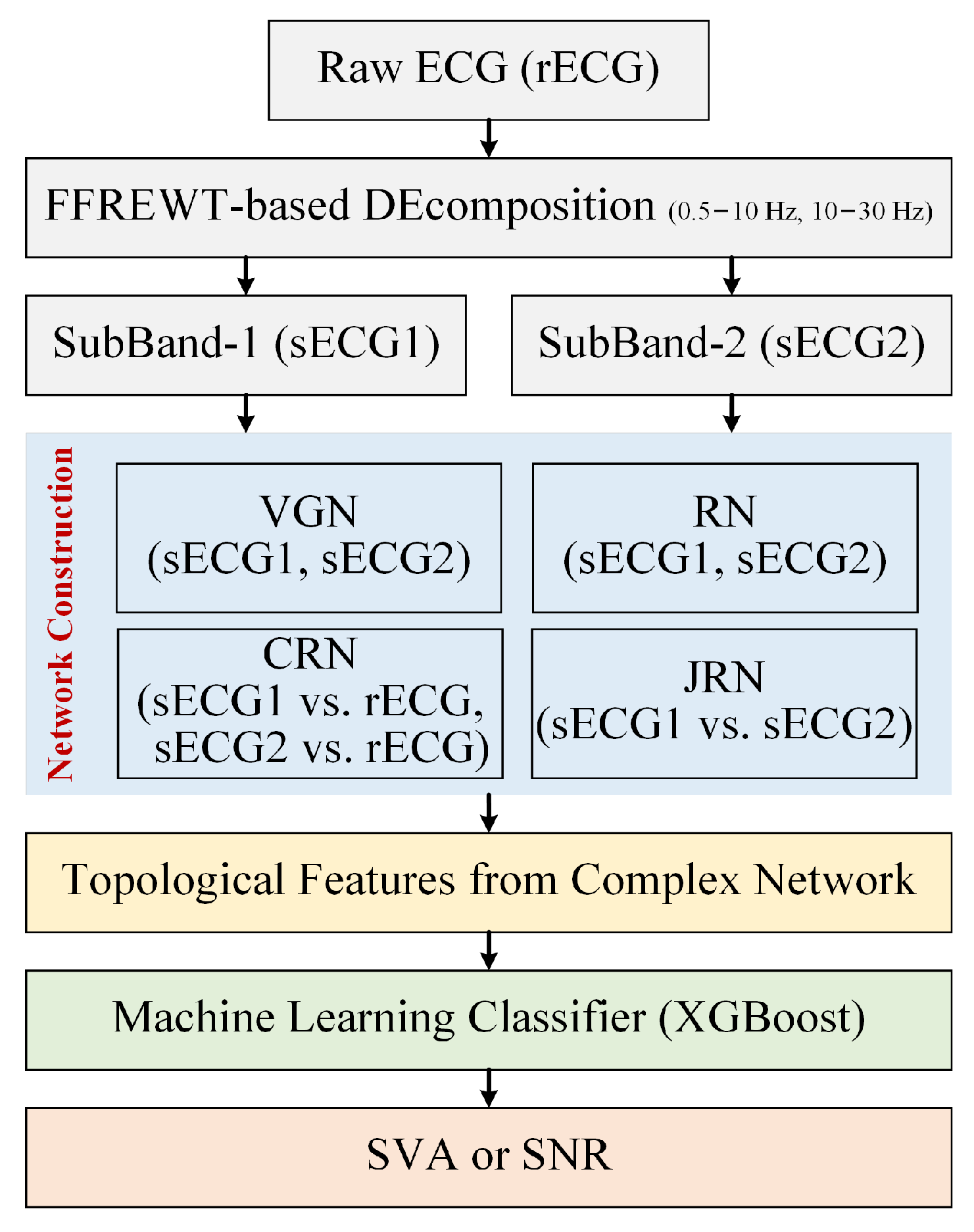
2.1.2. Signal Processing

The ECG signals from both databases were segmented into non-overlapping intervals based on respective labels (Figure 1). Segments identified as “Noise” were excluded to ensure data quality. The remaining segments were classified into two categories: SVA and NSR. SVA included segments corresponding to VT, VFL, and VF, all critical arrhythmias requiring prompt intervention. NSR encompassed a broader range of rhythms, such as normal sinus rhythm, atrial fibrillation, ventricular bigeminy, sinus bradycardia, first-degree heart block, high-grade ventricular ectopic activity, ventricular escape rhythm, and other rhythms not classified under SVA. To evaluate performance on short-term ECG signals, segments of varying durations (10, 8, 5, and 2 s) were analyzed (

Table 1. Number of ECG segments in different databases and datasets across varying segment lengths.

Database	Type	# 10 s Segment	# 8 s Segment	# 5 s Segment	# 2 s Segment
VFDB	NSR	3089	3882	6262	15,809
	SVA	748	951	1556	4022
CUDB	NSR	1284	1621	2642	6731
	SVA	303	391	660	1747
Train set	NSR	3935	4952	7932	20,286
	SVA	945	1207	1994	5192
Test set	NSR	438	551	882	2254
	SVA	106	135	222	577
Total	NSR	4373	5503	8814	22,540
	SVA	1051	1342	2216	5769

# means the number of each segment.

). This included 1051 SVA and 4373 NSR segments at 10 s, 1342 SVA and 5503 NSR segments at 8 s, 2216 SVA and 8814 NSR segments at 5 s, and 5769 SVA and 22,540 NSR segments at 2 s. To further enhance signal quality, a 0.5–40 Hz bandpass filter was applied to the segmented ECG fragments. This filtering process aimed to eliminate baseline drift and high-frequency noise, thereby providing clearer and more accurate ECG signals for subsequent analysis.

SVA and other heart rhythms exhibit distinct spectral characteristics. Previous studies have shown that SVA is associated with a notable reduction in spectral amplitude above 10 Hz. Based on this property, the fixed-frequency-range empirical wavelet transform (FFREWT) was selected for signal analysis [31]. The FFREWT was chosen because it can decompose signals into specific frequency bands while maintaining the integrity of the time-domain characteristics. Unlike other signal processing methods, the FFREWT is particularly effective at capturing localized frequency information across different scales, which is essential for identifying the subtle features associated with SVA. The ECG signals were decomposed into two targeted frequency bands: 0.5–10 Hz and 10–30 Hz. The 0.5–10 Hz band captures the low-frequency components, which are associated with overall heart activity and the underlying rhythm. The 10–30 Hz band focuses on higher-frequency components that may contain key information about arrhythmogenic events.

2.2. Complex Network Construction

2.2.1. Weighted Multi-Scale Visibility Graph

The visibility graph (VG) is a method used to transform a time series into a graph, making it possible to analyze complex temporal data using tools from graph theory. The VG algorithm was first introduced by Lacasa et al. [32] in 2008 and has since been applied in various fields such as physics, finance, biology, and more. In this study, each data point in the ECG time series is represented as a node in the network. The presence of edges between two nodes is determined by whether the corresponding data points meet specific visual criteria. Specifically, for two arbitrary data values $y_i$ and $y_j$ to be connected nodes of the associated graph, any other data value $y_k$ where $i<k<j$ must satisfy

$$y_k<y_i+{\displaystyle \frac{k-i}{j-i}}\times (y_j-y_i).$$

(1)

The VG algorithm assigns each data point in the time series to a node in the network, resulting in a substantial number of nodes and increased computational complexity of network features. To address this, coarse graining was employed to reduce signal complexity.

Moreover, in the VG algorithm, larger values indicate a broader visual field and typically a higher degree value. To underscore the significance of large values and retain more information during the coarse-grain transformation, Weighted Multi-Scale Visibility Graph (WMSVG) was adopted for constructing complex networks. This involves assigning greater weights to larger values and smaller weights to lower values.

For a time series $x_i$ of length N, the coarse-grained scale factor $\tau$ is defined to obtain the coarse-grained time series $y^{\left(\tau \right)}$:

$$y_j^{\left(\tau \right)}=\sum _{i=(j-1)\tau +1}^{j\tau }{w}_i{x}_i,$$

(2)

where $w_i$ is the weight of the value $x_i$ in the interval, which is usually set to be the ratio of the value to the sum of all values in the interval.

Then, a VG network (VGN) is constructed from the coarse-grained time series $y^{\left(\tau \right)}$ using the VG algorithm. WMSVG not only reduces the complexity of the network but also minimizes the loss of information from the original time series.

2.2.2. Recurrence Network

Recurrence networks (RNs) are an advanced method for analyzing the complex dynamics of time series data. They are based on the concept of recurrences in phase space, where a system’s state returns close to a previous state after some time. By representing these recurrences as a network, the underlying structure and behavior of the dynamical system can be studied through network theory.

The first step in constructing an RN is to reconstruct the phase space from a given time series into Recurrence Plots (RPs). For a univariate time series ${\left\{x\left(t_i\right)\right\}}_{i=1}^N$, the phase space is reconstructed using the method of time-delay embedding. The phase space vectors ${\mathbf{X}}_i$ are constructed as follows:

$${\mathbf{X}}_i=\left[x\left(t_i\right),x(t_i+\tau ),\dots ,x(t_i+(m-1)\tau )\right],$$

(3)

where m is the embedding dimension and $\tau$ is the time delay. The choice of m and $\tau$ is critical for accurately capturing the dynamics of the original system, and they are typically determined using techniques such as the False Nearest Neighbors method and mutual information.

Once the phase space is reconstructed, the next step is to calculate the distance between all pairs of phase space vectors. This is carried out by constructing a distance matrix $\mathbf{D}$, where each element $D_{ij}$ represents the distance between the vectors ${\mathbf{X}}_i$ and ${\mathbf{X}}_j$. The most common metric used is the Euclidean distance:

$$D_{ij}=|{\mathbf{X}}_i-{\mathbf{X}}_j|,$$

(4)

where $\parallel ·\parallel$ denotes the Euclidean norm. This distance matrix provides a quantitative measure of the proximity of the system’s states in the phase space.

A recurrence is defined by introducing a threshold $ϵ$. If the distance $D_{ij}$ between two states is less than or equal to $ϵ$, these states are considered recurrent, and an edge is established between the corresponding nodes in the network. This can be formally expressed as the adjacency matrix $\mathbf{A}$:

$$A_{ij}=\left\{\begin{array}{cc}1\hfill & \mathrm{if}{D}_{ij}\le ϵ,\hfill \\ 0\hfill & \mathrm{otherwise}.\hfill \end{array}\right.$$

(5)

Here, $A_{ij}$ is an element of the adjacency matrix, indicating whether a recurrence (and hence an edge) exists between the nodes i and j.

In this study, the original ECG signals and their sub-band components from two datasets were reconstructed into phase space. The resulting phase space trajectories were then converted into RPs for detailed analysis and comparison. The phase space reconstruction follows Han’s parameter settings [33], with the embedding dimension set to $m=3$ and the delay time to $\tau =3$. In converting the phase space states to RPs, the maximum norm was used to measure the distance between states, and the threshold for RN construction was set to 15% of the standard deviation of the time series. This approach ensures that the RPs effectively reveal the recurrence structures in the ECG signals.

2.2.3. Cross-Recurrence Network

A Cross-Recurrence Plot (CRP) [34] is an extension of RPs that analyzes the similarity between two systems by comparing their respective states. A CRP maps each state from the two time series into a point in high-dimensional space and identifies similar pairs within this space. Assuming the trajectory vectors of two systems in the m-dimensional phase space are $\mathbf{X}$ and $\mathbf{Y}$, the CRP can be represented by the matrix

$$C_{i,j}=\Theta (\epsilon -\parallel {\mathbf{X}}_i-{\mathbf{Y}}_j\parallel ),i=1,\dots ,N,j=1,\dots ,N$$

(6)

where $\Theta$ is the Heaviside function and $\epsilon$ is a threshold. After constructing the CRP, a cross-recurrence network (CRN) is created by treating the CRP as a binary adjacency matrix. Each state from both time series becomes a node, and an edge connects two nodes if their corresponding states are recurrent in phase space. This forms an undirected, unweighted network whose topological properties can be analyzed using complex network theory to explore dynamic interdependencies and coupling patterns between the two systems.

2.2.4. Joint Recurrence Network

A CRP is not suitable for analyzing two event sequences with different physical properties, as the differences between vectors with distinct physical units or phase space dimensions are not meaningful. In contrast, the Joint Recurrence Plot (JRP) examines recurrences within perspective phase space. It then identifies the time points when both systems simultaneously exhibit recurrence, referred to as joint recurrence points. The joint recurrence matrix for two systems can be represented as follows:

$$J_{i,j}=\Theta ({\epsilon }_1-\parallel {\mathbf{X}}_i-{\mathbf{Y}}_j\parallel )·\Theta ({\epsilon }_2-\parallel {\mathbf{X}}_i-{\mathbf{Y}}_j\parallel )$$

(7)

where $R_{{\epsilon }_1}(i,j)$ and $R_{{\epsilon }_2}(i,j)$ are the recurrence matrices for the two systems, with ${\epsilon }_1$ and ${\epsilon }_2$ being their respective thresholds and $\mathbf{X}$ and $\mathbf{Y}$ being the state trajectories of the two systems.

After the JRP is constructed, a joint recurrence network (JRN) is formed, where the JRP serves as a binary adjacency matrix. Each node represents a time point, and an edge connects two nodes if both systems show recurrence at those times. The resulting network is undirected and unweighted, reflecting the synchronized dynamics of the systems. Network measures can then reveal patterns of coordination and coupling between the systems.

2.3. Topological Feature Extraction from Complex Network

For a comprehensive analysis, eight network topology features were extracted from each network mapped from the sub-band signal: average degree, average path length, average clustering coefficient, transitivity, S-metric, graph energy, average closeness centrality, and average eigenvector centrality.

(a) Average Degree

The degree of a node, defined as the number of edges connected to it, is a fundamental measure of node connectivity. The average degree (aD) is computed as the mean degree of all nodes in the graph [35]:

$$\mathrm{aD}={\displaystyle \frac{1}{N}}\sum _{i=1}^N{k}_i$$

(8)

where N denotes the total number of nodes and $k_i$ is the degree of node i.

(b) Average Path Length

The shortest path between nodes serves as an indicator of transmission and communication efficiency within the graph. The average path length (aPL) is defined as the mean shortest path length between all pairs of nodes [36]:

$$\mathrm{aPL}={\displaystyle \frac{1}{\left|V\right|\left(\right|V|-1)}}\sum _{i\ne j}d(i,j)$$

(9)

where V represents the set of nodes, $d(i,j)$ is the shortest path from node i to node j, and $\left|V\right|$ is the total number of nodes in the graph.

(c) Average Clustering Coefficient

The clustering coefficient measures the likelihood that a node’s neighbors are also connected. For a node i, it is calculated as the ratio of the number of existing triangles involving node i to the maximum possible number of such triangles. The average clustering coefficient (aC) for the graph is the mean of the clustering coefficients of all nodes [35]:

$$\mathrm{aC}={\displaystyle \frac{1}{N}}\sum _{i=1}^N{C}_i$$

(10)

where $C_i={\displaystyle \frac{2e_i}{k_i(k_i-1)}}$, $e_i$ is the actual number of edges between the neighbors of node i, and $k_i$ is the degree of node i.

(d) Transitivity

Transitivity (Trans) quantifies the overall connectedness of the network, defined as the ratio of the number of triangles to the number of connected triples of nodes [35]:

$$\mathrm{Trans}={\displaystyle \frac{3\times \mathrm{Number}\mathrm{of}\mathrm{triangles}}{\mathrm{Number}\mathrm{of}\mathrm{connected}\mathrm{triples}\mathrm{of}\mathrm{nodes}}}$$

(11)

(e) S-metric

The S-metric (sM) provides information about the network’s connectivity efficiency, calculated as the sum of the products of nodal degrees for all edges [37]:

$$\mathrm{sM}=\sum _{(i,j)\in E}{k}_i{k}_j$$

(12)

where E is the set of edges and $k_i,k_j$ are the degrees of nodes i and j, respectively.

(f) Graph Energy

Graph energy (GE) is a spectral graph measure defined as the sum of the absolute values of the real components of the eigenvalues of the adjacency matrix [38]:

$$\mathrm{GE}=\sum _{i=1}^N\left|{\lambda }_i\right|$$

(13)

where ${\lambda }_i$ are the eigenvalues of the adjacency matrix of the graph.

(g) Average Eigenvector Centrality

Eigenvector centrality assesses the influence of a node in terms of its connections to other nodes. It is represented by the eigenvector corresponding to the largest eigenvalue of the adjacency matrix. The average eigenvector centrality (aEC) is the mean value of the eigenvector centralities for all nodes [39]:

$$\mathrm{aEC}={\displaystyle \frac{1}{N}}\sum _{i=1}^N{x}_i$$

(14)

where $x_i$ is the eigenvector centrality of node i and ${\lambda }_{\max }$ is the largest eigenvalue of the adjacency matrix A.

2.4. Machine Learning Classifier and Evaluation Metrics

XGBoost is recognized as an optimized distributed boosting library, highly valued for its superior accuracy, robust flexibility, and inherent capability to prevent overfitting. In this study, eight features are extracted from each of the four sub-band signals, which are obtained through the FFREWT. The resulting feature matrix, incorporating features from both sub-bands, is subsequently input into the XGBoost classifier for signal segment classification.

To assess the efficacy of the proposed method in distinguishing SVA from NSR, a 10-fold cross-validation approach is employed. The data is divided into ten subsets. In each iteration, nine are used for training and one for validation, ensuring a comprehensive evaluation over ten cycles. To address the issue of data imbalance, which can adversely affect model performance, the Synthetic Minority Over-sampling Technique is applied to balance the data within each fold of the cross-validation process.

The performance of the proposed algorithm is evaluated using three widely adopted standard statistical parameters: sensitivity (Se), specificity (Sp), and accuracy (Acc). These metrics are computed as follows, where $TP$, $TN$, $FP$, and $FN$ represent true positives, true negatives, false positives, and false negatives, respectively:

$$\mathrm{Se}={\displaystyle \frac{TP}{TP+FN}}$$

(15)

$$\mathrm{Sp}={\displaystyle \frac{TN}{TN+FP}}$$

(16)

$$\mathrm{Acc}={\displaystyle \frac{TP+TN}{TP+TN+FP+FN}}$$

(17)

3. Results

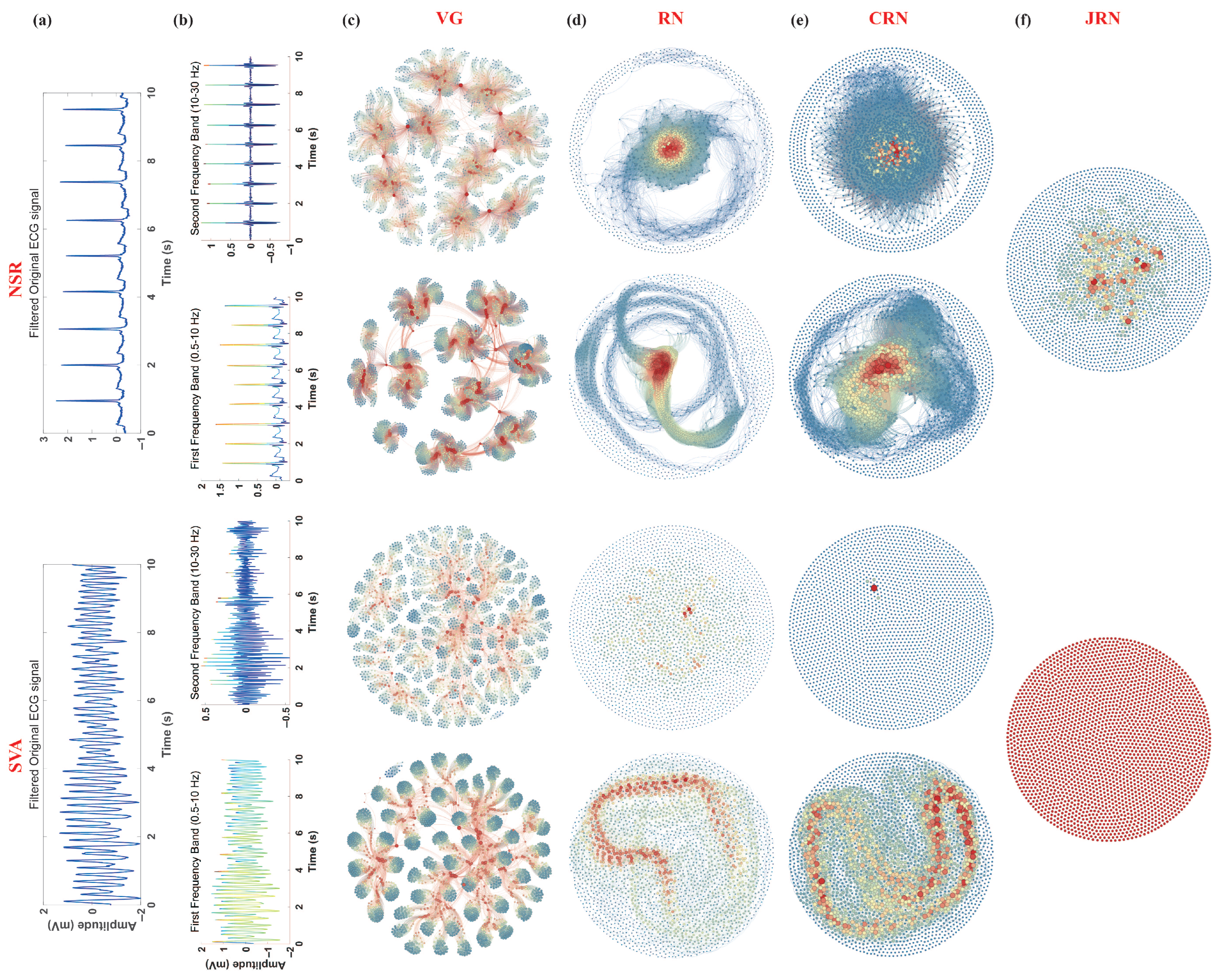
3.1. Complex Network Comparison for SVA/NSR Segments

In this study, two frequency bands of 10 s segments of two types of ECG signals were mapped into visual graph networks. Figure 2a presents the typical waveforms of SVA and NSR, along with their decomposed sub-signals (Figure 2b). Figure 2c–f display the corresponding networks for these sub-signals. The network graphs were generated using the open-source software “Gephi-0.10” with the “Fruchterman-Reingold” layout. Nodes with different degree values are colored differently, corresponding to the colors of data points in the sub-signals. Additionally, the size of each node in the network graph reflects its degree value. Nodes with higher degree values are represented by larger node sizes in the network graph.

3.1.1. VGN

From Figure 2c, it is evident that, compared to SVA, the network nodes mapped from sub-signals of NSR in each frequency band generally exhibit higher degree values. This observation arises because the visual graph construction method enables extremum points in the time series to “see” a greater number of points in the series, resulting in corresponding nodes with higher degrees in the network. The sub-signals of both frequency bands for NSR display pronounced R-peaks, with most data points outside the R-peaks residing near the baseline. Consequently, data points at the R-peaks are visible to more points and thus exhibit higher degree values. Nodes between two R-peaks are densely interconnected in the network, forming distinct clusters. Each cluster is connected by a high-degree node corresponding to an R-peak in the time series.

In contrast, the sub-signal of SVA in the 0.5–10 Hz band resembles a sinusoidal signal; although its amplitude is unstable, it contains many local extremum points. Similar to NSR, most data points between two local maxima are visible. However, due to the rapid rhythm of SVA, fewer data points exist between two local maxima compared to NSR, resulting in nodes with lower degree values and the formation of more clusters in the network graph. For a 10 s ECG segment at a sampling rate of 250 Hz, in the network mapped from the 0.5–10 Hz band sub-signal, most nodes associated with SVA have a degree value less than 60, whereas many nodes in networks corresponding to NSR exhibit degree values exceeding 80 or even 100.

The energy for SVA is mainly concentrated in the 0.5–10 Hz band. In contrast, the 10–30 Hz sub-band is highly disordered, with minimal energy and loss of rhythmic ECG patterns, which is reflected in the chaotic structure of the corresponding network graph. Conversely, NSR maintains clear R-peaks in the 10–30 Hz band, leading to the formation of distinct node clusters in the corresponding network graphs. The number of clusters corresponds to the number of R-R intervals in the analyzed ECG frequency band, highlighting significant differences in the complexity of networks corresponding to the two types of ECGs.

3.1.2. RN

From Figure 2d, the structural differences in RN mapped from NSR and SVA ECG sub-signals are readily apparent. The RN constructed from NSR sub-band signals shows a highly centralized structure. Nodes corresponding to R-peaks have high degree values and form dense clusters near the network center. These clusters reflect the periodic and regular nature of NSR signals, as similar states in the time series recur at regular intervals. In contrast, the RN mapped from SVA sub-signals is more scattered, with irregular and less connected clusters due to the rapid and unstable rhythm of SVA. Particularly in the 0.5–10 Hz band, although local clusters form around transient extremum points, the overall network is fragmented, with significantly fewer high-degree nodes compared to NSR. The network derived from the 10–30 Hz band of SVA shows a highly dispersed, almost random structure, indicating the loss of recurrence characteristics at higher frequencies. This reflects the fundamental difference in temporal dynamics and recurrence properties between NSR and SVA signals, effectively captured by the RN framework.

3.1.3. CRN

Figure 2e shows that the CRN exhibits distinct patterns. These patterns reflect the similarity and coupling strength between sub-band signals. For NSR, the CRN appears densely connected. Clusters are clearly formed, and nodes related to R-peaks in both bands show strong mutual recurrence. The dense clustering indicates strong inter-band correlation. This is attributed to the stable and repetitive characteristics of normal sinus rhythm. The number of visible clusters in the NSR CRN typically aligns with the number of R-R intervals, illustrating the consistent recurrence structure across frequencies. Conversely, the CRN in SVA displays a looser and fragmented network with noticeably fewer high-degree nodes. Some small clusters appear at moments of transient correlation. However, the rapid and irregular rhythm in SVA disrupts the stability of recurrence between frequency bands. Especially in the 10–30 Hz range, the recurrence structure is nearly lost. This indicates a significant breakdown of coupling and dynamic consistency between frequency bands in SVA, highlighting its pathological signal characteristics.

3.1.4. JRN

Figure 2f presents the JRN, which combines the recurrence properties of both sub-signals from different frequency bands by identifying simultaneous recurrences in both. In NSR, the JRN displays a well-organized structure where clusters of highly interconnected nodes reflect synchronized recurrence events across both frequency bands. High-degree nodes within these clusters correspond to the R-peaks, which remain prominent features in both sub-bands, thereby reinforcing joint dynamic recurrence. The regular R-R intervals in NSR contribute to the formation of these consistent clusters, resulting in a compact and well-organized JRN topology. In contrast, the JRN of SVA is sparse and poorly structured, particularly in the 10–30 Hz band where joint recurrences are almost nonexistent due to the irregularity of high-frequency components. In the 0.5–10 Hz band, limited clustering is observed. Although the rapid fluctuations of SVA allow for occasional joint recurrence, the overall network remains fragmented. This visualization highlights the significant difference in multiscale recurrence synchronization between NSR and SVA signals.

3.2. Investigation of Frequency Band Significance

Table 2. Classification results of network features corresponding to sub-signals in different frequency bands.

Features	Se (%)	Sp (%)	Acc (%)
VGN1	88.64 ± 1.44	88.75 ± 1.33	88.65 ± 0.03
VGN2	94.87 ± 0.99	94.91 ± 1.40	94.86 ± 0.02
RN1	97.13 ± 0.62	97.59 ± 0.77	97.38 ± 0.03
RN2	96.29 ± 1.46	96.26 ± 1.65	96.24 ± 0.01
CRN1	98.24 ± 1.04	97.30 ± 1.10	97.79 ± 0.01
CRN2	92.96 ± 0.80	94.78 ± 0.31	93.92 ± 0.04

provides a comparative analysis of classification results. It focuses on network features extracted from sub-signals in different frequency bands, including those based on VGN, RN, and CRN models. VGN1 and VGN2 represent features from two frequency bands of the VGN, RN1 and RN2 from the RN, and CRN1 and CRN2 from the CRN. Among the features, CRN1 exhibits the highest performance, demonstrating superior Se = 98.24 ± 1.04%, Sp = 97.30 ± 1.10%, and Acc = 97.79 ± 0.01%. These results highlight its effectiveness in capturing complex patterns within sub-signals. In contrast, VGN1 has the lowest classification results (Se = 88.64 ± 1.44%, Sp = 88.75 ± 1.33%, and Acc = 88.65 ± 0.03%), indicating less efficacy in accurately identifying and classifying the sub-signals. The analysis highlights the varying effectiveness of different network features, with CRN features being particularly effective in improving classification accuracy. This suggests that CRN networks can effectively capture complex interactions between sub-signals across different frequency bands, making them useful for precise signal analysis. Meanwhile, the performance gap between VGN1 and other features suggests a need for further refinement or alternative feature extraction methods to improve its effectiveness.

For each network type (VGN1, VGN2, RN1, RN2, CRN1, CRN2, and JRN), we extracted the values of seven network features, including aD, aPL, aCC, Trans, sM, GE, and aEC, from all time series samples. Then, for each feature within each network type, a Kruskal–Wallis test was performed to assess whether the distributions of feature values significantly differed between NSR and SVA. Figure 3 summarizes the p-values obtained from these tests, indicating the discriminative ability of each feature for distinguishing NSR and SVA data under different network representations. Each circle in the matrix represents a p-value. Its color and size reflect the value: larger and redder circles indicate lower p-values (stronger significance), whereas smaller and bluer circles correspond to higher p-values (weaker significance). The majority of p-values fall within the highly significant range (p ≤ 0.01), suggesting that most features exhibit statistically significant differences among groups. Features such as aD, aPL, aCC, and GE demonstrate consistent significance across nearly all groups, highlighting their robustness and potential importance in downstream analyses or classification tasks. In contrast, the feature Trans shows relatively higher p-values in CRN1 (p = 0.335) and CRN2 (p = 0.080), indicating a lack of statistical significance in these contexts. Similarly, aEC does not reach statistical significance in VG1 (p = 0.160), whereas in CRN2 it is only marginally significant (p = 0.019).

3.3. Ablation Experiment for Complex Network Importance Evaluation

Table 3. Classification results using different network features.

Features	Se (%)	Sp (%)	Acc (%)
VGN	97.22 ± 1.39	96.69 ± 1.41	97.00 ± 0.02
RN	98.35 ± 0.58	98.08 ± 0.72	98.26 ± 0.02
CRN	98.10 ± 0.79	97.62 ± 0.56	97.82 ± 0.02
JRN	96.65 ± 1.26	94.76 ± 1.42	95.65 ± 0.01
VGN + RN	97.95 ± 1.18	97.75 ± 1.10	97.80 ± 0.01
VGN + CRN	98.73 ± 0.71	97.97 ± 0.76	98.31 ± 0.01
VGN + JRN	97.39 ± 1.01	97.59 ± 0.87	97.55 ± 0.03
RN + CRN	98.97 ± 0.49	98.11 ± 0.54	98.59 ± 0.01
RN + JRN	98.31 ± 1.11	98.05 ± 1.17	98.11 ± 0.01
CRN + JRN	98.48 ± 0.70	98.18 ± 0.80	98.36 ± 0.02
VGN + RN + CRN	98.28 ± 0.92	98.56 ± 1.07	98.49 ± 0.01
VGN + RN + JRN	98.21 ± 0.72	97.01 ± 0.52	97.53 ± 0.02
VGN + CRN + JRN	98.17 ± 0.51	98.27 ± 0.38	98.23 ± 0.01
RN + CRN + JRN	99.03 ± 0.08	98.00 ± 0.09	98.41 ± 0.01
All	99.02 ± 0.53	99.17 ± 0.43	98.73 ± 0.02

demonstrates the classification performance in various network features, including VGN, RN, CRN, and JRN. These features are evaluated individually and in different combinations, with Se, Sp, and Acc as key metrics.

When characteristics are individually analyzed, RN has the highest performance, achieving an Se of 98.35 ± 0.58%, an Sp of 98.08 ± 0.72%, and an accuracy of 98.26 ± 0.02%. This indicates that RN is particularly effective in capturing the intrinsic patterns of the data, making it the most reliable single feature for classification tasks. CRN also performs well, with an accuracy of 97.82 ± 0.02%, slightly lower than RN. Although VGN performs slightly worse than both RN and CRN, it still maintains an accuracy of 97.00 ± 0.02%. JRN shows the lowest performance among individual characteristics, with an accuracy of 95.65 ± 0.01%, suggesting that it may not be as powerful when used alone.

When two features are combined, the combination of RN and CRN yields the best results, with an accuracy of 98.59 ± 0.01%, indicating a strong relationship between these two features. The combination of VGN and CRN also performs well, with an accuracy of 98.31 ± 0.01%, slightly surpassing the VGN and RN combination. This implies that CRN’s capabilities in detecting cross-recurrences add significant value when paired with other features.

The combination of three features (VGN+RN+CRN) achieves the highest accuracy at 98.49 ± 0.01%, closely followed by RN + CRN + JRN, which also attains 98.41 ± 0.01%. These results underscore the synergistic effects of combining multiple features, where each feature contributes to a more nuanced understanding of the data, leading to enhanced classification performance.

Finally, when all four features (VGN + RN + CRN + JRN) are combined, the classification accuracy reaches its peak at 99.02 ± 0.53%, with an Se of 99.17 ± 0.43% and Sp of 98.73 ± 0.02%. This demonstrates the advantages of integrating diverse network features, as the combination leverages the strengths of each individual feature, resulting in a model that is more robust and reliable in handling complex data structures.

3.4. Performance of the Proposed Method on Short-Term ECG

Table 4. Detection performance and mobile deployment efficiency of SVA across varying ECG segment lengths.

Segment Length (s)	Features	Se (%)	Sp (%)	Acc (%)	Mean Running Time (ms)	Mean Energy Consumption (mWh)
10	VGN-related	97.22 ± 1.39	96.69 ± 1.41	97.00 ± 0.02	228	0.035
	RN-related	99.03 ± 0.08	98.00 ± 0.09	98.41 ± 0.01	356	0.048
	All	99.02 ± 0.53	98.44 ± 0.43	98.73 ± 0.02	667	0.095
8	VGN-related	96.74 ± 0.09	96.66 ± 0.09	96.68 ± 0.03	185	0.028
	RN-related	97.49 ± 0.74	98.95 ± 0.63	98.21 ± 0.01	297	0.043
	All	98.06 ± 1.29	98.67 ± 1.16	98.29 ± 0.01	502	0.078
5	VGN-related	95.57 ± 0.35	95.54 ± 0.34	95.60 ± 0.04	121	0.018
	RN-related	97.56 ± 1.04	98.36 ± 0.87	97.91 ± 0.01	184	0.023
	All	98.48 ± 0.66	98.00 ± 0.44	98.21 ± 0.01	346	0.054
2	VGN-related	90.75 ± 1.37	92.30 ± 0.97	91.67 ± 0.01	34	0.008
	RN-related	97.43 ± 1.10	95.54 ± 1.07	96.54 ± 0.01	58	0.011
	All	97.23 ± 0.76	95.85 ± 0.95	96.62 ± 0.02	97	0.021

summarizes the SVA detection performance across different ECG segment lengths using various feature extraction strategies. The results demonstrate that combining features from multiple complex network types (All) consistently achieves better performance than using features derived from a single network type, regardless of the segment duration. Moreover, among the individual network categories, features extracted from multivariate recurrence-based networks (RN-related), including RN, CRN and JRN, outperform those obtained from visibility graph-based networks (VGN-related), highlighting the advantage of RN-related representations in capturing discriminative information for SVA detection.

Although RN-related methods demonstrate high specificity, adding VGN features provides only little improvement in this metric. However, the combined features substantially enhance sensitivity, which is crucial for the accurate detection of SVA. Since misclassifying arrhythmias as NSR can lead to serious clinical consequences, improving sensitivity is especially crucial in real-world applications.

As the ECG segment length decreases, the performance of all methods declines. This is especially notable for VGN-related features when the ECG segment length is reduced from 5 to 2 s. It is likely because shorter segments fail to capture the global dynamics of cardiac activity adequately. Additionally, although the time series coarsening used in constructing multi-band VGN features intended to reduce computational complexity, it may also degrade feature quality.

In contrast, RN-related methods demonstrate greater stability in different segment lengths, as they primarily capture local dynamic characteristics of the signal and rely less on extended temporal information. Both Se and Sp for RN-related features remain relatively consistent, with only a slight decline observed at the 2 s segment length (Se decreases by 0.13%, Sp by 2.82%, and Acc by 1.37%).

The method combining multiple features also shows decreased performance with shorter segments but remains slightly more robust than RN alone. This indicates that integrating features from multiple networks helps preserve diagnostic accuracy in shorter ECG recordings.

3.5. Mobile Deployment of the Proposed Model

In this study, the XGBoost model trained using Python-3.9 has been successfully deployed to an Android mobile platform (Figure 4). Initially, the trained model was serialized into a *.pkl file using the joblib library. To ensure compatibility with mobile environments, the model was subsequently converted into the ONNX (Open Neural Network Exchange) format. On the Android side, an application framework was developed using Java within the Android Studio environment, and ONNX Runtime for Mobile was integrated to enable model loading and inference.

All processing procedures, including signal preprocessing (such as filtering and FFPREWT), feature extraction, and classification, are performed directly on the mobile device without relying on any external server or cloud services. These processing modules were implemented in Java and C++ (via the Android NDK where appropriate) to optimize computational efficiency. To further enhance real-time performance, model quantization and system-level adjustments were applied for the Android operating system.

We evaluated the deployment by measuring inference latency and energy consumption on the mobile device for ECG segments of varying lengths. Table 4 summarizes the detection performance, mean running time, and average energy consumption per inference. The average inference time ranges from 97 ms for 2 s segments to 667 ms for 10 s segments, demonstrating fast on-device processing suitable for real-time applications. Energy consumption was measured using the Android Battery Historian tool, which monitored total power usage during inference over the full test set. The mean energy consumption per inference varied between 0.008 mWh and 0.095 mWh depending on segment length and feature set complexity. These results confirm that the deployment achieves efficient inference with low power consumption, balancing accuracy, latency, and energy efficiency for practical mobile health monitoring.

4. Discussion

4.1. Comparison with Existing Methods

Table 5. Comparison of the proposed method with existing methods for SVA detection.

Author	Method	Segment Length (s)	Se (%)	Sp (%)	Acc (%)
Panda [45]	FFREWT + CNN	8	99.95	95.95	99.04
Verma [47]	Features + RF	8	95.17	97.32	97.17
Cheng [40]	Features + SVM	8	93.87	95.56	95.46
Nguyen [41]	Features + SVM	5	90.8	96.90	95.70
Tripathy [48]	Taylor–Fourier Transform + Phase Difference + SVM	5	82.61	79.57	80.99
Xu [43]	VMD + Boosting-CART	5	97.32	98.95	98.29
Lai [44]	2D-CNN	3	95.05	99.43	98.82
Acharya [46]	CNN	2	95.32	91.04	93.18
Our	FFREWT + Multiple Complex Networks + XGBoost	10	99.02 ± 0.53	98.44 ± 0.43	98.73 ± 0.02
		8	98.06 ± 1.29	98.67 ± 1.16	98.29 ± 0.01
		5	98.48 ± 0.66	98.00 ± 0.44	98.21 ± 0.01
		2	97.23 ± 0.76	95.85 ± 0.95	96.62 ± 0.02

highlights a comparative analysis between the proposed method in this study and existing approaches for detecting SVA, with a focus on ECG segment length and key performance metrics such as Se, Sp, and Acc. The proposed method, which combines the FFREWT, VG networks, multivariate RPs, and XGBoost, demonstrates exceptional performance without the need for prior R-wave detection. Compared to traditional feature-based methods used by authors like Cheng et al. [40] and Nguyen et al. [41], which rely on time-domain, frequency-domain, and complexity features, the proposed method exhibits superior detection capabilities. These traditional methods often struggle to capture the intricate dynamics of ECG signals, resulting in lower Se and Sp. In contrast, the proposed approach effectively leverages complex network features to reveal underlying ECG information, enhancing interpretability and classification accuracy. Sharma et al. [42] and Xu et al. [43] use signal decomposition methods to achieve performance metrics comparable to those of the proposed method. However, their approach is limited in scope, considering only a narrow range of arrhythmias beyond SVA, such as normal sinus rhythm and ventricular ectopic beats. In contrast, the proposed method encompasses a broader spectrum of cardiac rhythms, demonstrating its versatility and comprehensive diagnostic capability. Deep learning methods, particularly CNNs demonstrated by Lai et al. [44], Panda et al. [45], and Acharya et al. [46], often achieve high performance in arrhythmia detection. However, these models typically find it difficult to understand the decision-making process due to the lack of interpretability. The proposed method addresses this by offering competitive classification performance and enhanced interpretability. Through complex network features, the method reveals properties of ECG signals and provides valuable insights into arrhythmic patterns.

4.2. Influence of Frequency Band Characteristics on Detection Performance

When applying multi-band complex networks to detect SVA, VGN-based and RN-based methods show distinct performance across frequency bands, rooted in their inherent mechanisms and alignment with physiological information in specific ranges. VGN builds networks by assessing the “visibility” of extremum points in time series, where nodes linked to prominent peaks or valleys (such as R-peaks) connect to more adjacent points, resulting in higher node degrees and denser clusters. This makes VGN highly sensitive to the morphological clarity of sharp, transient ECG features. The 10–30 Hz band, despite having fewer low-frequency components, retains distinct QRS complex features—particularly R-peaks—in NSR. These R-peaks act as strong extremum points, allowing their corresponding VGN nodes to form well-defined clusters that effectively differentiate NSR from SVA. In contrast, SVA in the 10–30 Hz band displays chaotic, low-energy patterns with blurred or absent R-peaks, leading to fragmented VGN structures with fewer high-degree nodes, explaining VGN’s superior performance in this range.

RN, on the other hand, analyzes dynamic recurrence of physiological states through phase space reconstruction, focusing on the temporal regularity of cardiac cycles like the periodic recurrence of P waves, QRS complexes, and T waves. This makes RN more sensitive to the rhythmicity and consistency of long-term physiological patterns than isolated morphological features. The 0.5–10 Hz band encompasses key ECG physiological features, including the complete cardiac cycle. For NSR, these features show stable, periodic recurrence in phase space, forming centralized RN clusters reflecting regular cardiac dynamics. For SVA, the 0.5–10 Hz band retains residual rhythmic activity, whose recurrent patterns (or absence) RN can detect to distinguish SVA from NSR. The 10–30 Hz band for SVA lacks such recurrence, dominated by high-frequency noise, reducing RN’s effectiveness, thus explaining its better performance in the 0.5–10 Hz range.

Combining features from both bands outperforms using the original signal alone, as they capture complementary information: 0.5–10 Hz preserves global rhythmic dynamics, while 10–30 Hz highlights local morphological details. Their integration leverages both networks’ strengths, providing a more comprehensive ECG characterization and enhancing SVA detection robustness.

4.3. Effect of ECG Segment Length on Detection Accuracy

The analysis of Table 4 highlights the influence of ECG segment length on the performance of SVA detection using different network features. The table shows that as the segment length decreases from 10 s to 8 s and 5 s, there is only a slight decline in classification performance across all feature sets, including VGN-related and RN-related features and the combination of all features. Specifically, the overall Acc and Se remain stable with only minor reductions. However, performance notably declines when the segment length is reduced to 2 s. For instance, VGN features show a significant decrease in Se from 97.22 ± 1.39% at 10 s to 90.75 ± 1.37% at 2 s, and Acc decreases from 97.00 ± 0.02% to 91.67 ± 0.01%. This reduction is also reflected in the RN-related and all feature sets, with Acc dropping slightly from 98.41 ± 0.01% at 10 s to 96.54 ± 0.01% at 2 s for all features.

The notable performance decrease at the 2 s segment length can be attributed to the limited amount of ECG data within such a short time frame. A 2 s segment usually contains only a single R-wave, often positioned centrally within the segment. As a result, the points on either side of the R-peak are connected to fewer points, reducing the degree values for many nodes in the network and altering the clustering structure. This disruption in network topology diminishes the effectiveness of several key features related to node degree and clustering coefficient, which are crucial for accurate classification. Although the reduction in ECG data leads to a decrease in the utility of network-derived features, posing a challenge to SVA identification based on 2 s segments, the proposed method maintains robust performance across a variety of segment lengths. This suggests that segment length is important for the accuracy of SVA detection, especially when adopting network-based feature extraction methods.

4.4. Limitations and Future Directions

This study has limitations that need to be acknowledged. Firstly, the absence of real-world clinical data for algorithm testing is a notable constraint. The reliance solely on publicly available database data for model training and testing may affect the generalizability of the results to diverse clinical scenarios. Additionally, the scope of this study is restricted to distinguishing between SVA and NSR, without delving into more nuanced classifications of beats or rhythms. Future research could benefit from incorporating diverse and authentic clinical datasets to enhance the robustness and applicability of the proposed algorithm. Furthermore, exploring better classifications of cardiac rhythms could provide more comprehensive insights into the performance of the algorithm across a broader spectrum of cardiovascular events.

5. Conclusions

This study presents a novel multi-band, multi-network approach for detecting life-threatening ventricular arrhythmias using short-term single-lead ECG signals. By decomposing ECG data via the FFREWT and constructing VGN, RN, CRN, and JRN networks across different frequency bands, both temporal and spectral dynamics can be effectively captured in inherent arrhythmic patterns. The extracted topological features, combined through an XGBoost classifier, deliver superior detection accuracy and sensitivity compared to conventional and deep learning-based methods, particularly when handling short ECG segments. Additionally, the approach demonstrates robustness across varying signal durations and offers valuable interpretability of the complex dynamics of ECG signals, addressing key limitations of existing black-box models. The successful deployment of the classifier on an Android platform further validates its feasibility for real-time, wearable applications. Future work will focus on expanding the classification scope to finer rhythm categories and validating the method on diverse clinical ECG datasets to enhance its generalizability in real-world scenarios.

References

1. Marijon, E.; Narayanan, K.; Smith, K.; Barra, S.; Basso, C.; Blom, M.T.; Crotti, L.; D’Avila, A.; Deo, R.; Dumas, F.; et al. The Lancet Commission to Reduce the Global Burden of Sudden Cardiac Death: A Call for Multidisciplinary Action. Lancet 2023, 402, 883–936. [Google Scholar] [CrossRef]
2. Deyell, M.W.; Krahn, A.D.; Goldberger, J.J. Sudden Cardiac Death Risk Stratification. Circ. Res. 2015, 116, 1907–1918. [Google Scholar] [CrossRef]
3. Trancuccio, A.; Kukavica, D.; Sugamiele, A.; Mazzanti, A.; Priori, S.G. Prevention of Sudden Death and Management of Ventricular Arrhythmias in Arrhythmogenic Cardiomyopathy. Card. Electrophysiol. Clin. 2023, 15, 349–365. [Google Scholar] [CrossRef] [PubMed]
4. Hammad, M.; Iliyasu, A.M.; Subasi, A.; Ho, E.S.L.; El-Latif, A.A.A. A Multitier Deep Learning Model for Arrhythmia Detection. IEEE Trans. Instrum. Meas. 2021, 70, 1–9. [Google Scholar] [CrossRef]
5. Kolk, M.Z.H.; Frodi, D.M.; Langford, J.; Jacobsen, P.K.; Risum, N.; Andersen, T.O.; Tan, H.L.; Hastrup Svendsen, J.; Knops, R.E.; Diederichsen, S.Z.; et al. Artificial Intelligence-Enhanced Wearable Technology Enables Ventricular Arrhythmia Prediction. Eur. Heart J.—Digit. Health 2024, ztae069. [Google Scholar] [CrossRef]
6. Lee, S.; Park, D. Improved Dynamic Programming in Local Linear Approximation Based on a Template in a Lightweight ECG Signal-Processing Edge Device. J. Inf. Process. Syst. 2022, 18, 97–114. [Google Scholar] [CrossRef]
7. Matsuura, N.; Kuwabara, K.; Ogasawara, T. Lightweight Heartbeat Detection Algorithm for Consumer Grade Wearable ECG Measurement Devices and Its Implementation. In Proceedings of the 2022 44th Annual International Conference of the IEEE Engineering in Medicine & Biology Society (EMBC), Glasgow, Scotland, UK, 11–15 July 2022; pp. 4299–4302. [Google Scholar] [CrossRef]
8. Shen, Q.; Li, J.; Cui, C.; Wang, X.; Gao, H.; Liu, C.; Chen, M. A Wearable Real-Time Telemonitoring Electrocardiogram Device Compared with Traditional Holter Monitoring. J. Biomed. Res. 2021, 35, 238. [Google Scholar] [CrossRef]
9. Rauf, S.; Bilal, R.M.; Li, J.; Vaseem, M.; Ahmad, A.N.; Shamim, A. Fully Screen-Printed and Gentle-to-Skin Wet ECG Electrodes with Compact Wireless Readout for Cardiac Diagnosis and Remote Monitoring. ACS Nano 2024, 18, 10074–10087. [Google Scholar] [CrossRef]
10. Pantelidis, P.; Dilaveris, P.; Ruipérez-Campillo, S.; Goliopoulou, A.; Giannakodimos, A.; Theofilis, P.; De Lucia, R.; Katsarou, O.; Zisimos, K.; Kalogeras, K.; et al. Hearts, Data, and Artificial Intelligence Wizardry: From Imitation to Innovation in Cardiovascular Care. Biomedicines 2025, 13, 1019. [Google Scholar] [CrossRef]
11. Page, R.L.; Joglar, J.A.; Caldwell, M.A.; Calkins, H.; Conti, J.B.; Deal, B.J.; Estes, N.M.; Field, M.E.; Goldberger, Z.D.; Hammill, S.C.; et al. 2015 ACC/AHA/HRS Guideline for the Management of Adult Patients With Supraventricular Tachycardia. J. Am. Coll. Cardiol. 2016, 67, e27–e115. [Google Scholar] [CrossRef]
12. Aktaa, S.; Tzeis, S.; Gale, C.P.; Ackerman, M.J.; Arbelo, E.; Behr, E.R.; Crotti, L.; d’Avila, A.; De Chillou, C.; Deneke, T.; et al. European Society of Cardiology Quality Indicators for the Management of Patients with Ventricular Arrhythmias and the Prevention of Sudden Cardiac Death. EP Eur. 2023, 25, 199–210. [Google Scholar] [CrossRef]
13. Niu, Y.; Wang, H.; Wang, H.; Zhang, H.; Jin, Z.; Guo, Y. Diagnostic Validation of Smart Wearable Device Embedded with Single-Lead Electrocardiogram for Arrhythmia Detection. Digit. Health 2023, 9, 20552076231198682. [Google Scholar] [CrossRef]
14. Kim, D.; Min, J.; Ko, S.H. Recent Developments and Future Directions of Wearable Skin Biosignal Sensors. Adv. Sens. Res. 2024, 3, 2300118. [Google Scholar] [CrossRef]
15. Yu, S.; Liu, S. A Novel Adaptive Recursive Least Squares Filter to Remove the Motion Artifact in Seismocardiography. Sensors 2020, 20, 1596. [Google Scholar] [CrossRef] [PubMed]
16. Volak, J.; Bajzik, J.; Janisova, S.; Koniar, D.; Hargas, L. Real-Time Interference Artifacts Suppression in Array of ToF Sensors. Sensors 2020, 20, 3701. [Google Scholar] [CrossRef] [PubMed]
17. Martis, R.J.; Acharya, U.R.; Min, L.C. ECG Beat Classification Using PCA, LDA, ICA and Discrete Wavelet Transform. Biomed. Signal Process. Control 2013, 8, 437–448. [Google Scholar] [CrossRef]
18. Sabut, S.; Pandey, O.; Mishra, B.S.P.; Mohanty, M. Detection of Ventricular Arrhythmia Using Hybrid Time–Frequency-Based Features and Deep Neural Network. Phys. Eng. Sci. Med. 2021, 44, 135–145. [Google Scholar] [CrossRef]
19. Saini, S.K.; Gupta, R. Artificial Intelligence Methods for Analysis of Electrocardiogram Signals for Cardiac Abnormalities: State-of-the-Art and Future Challenges. Artif. Intell. Rev. 2022, 55, 1519–1565. [Google Scholar] [CrossRef]
20. Jha, C.K.; Kolekar, M.H. Cardiac Arrhythmia Classification Using Tunable Q-wavelet Transform Based Features and Support Vector Machine Classifier. Biomed. Signal Process. Control 2020, 59, 101875. [Google Scholar] [CrossRef]
21. Acharya, U.R.; Oh, S.L.; Hagiwara, Y.; Tan, J.H.; Adam, M.; Gertych, A.; Tan, R.S. A Deep Convolutional Neural Network Model to Classify Heartbeats. Comput. Biol. Med. 2017, 89, 389–396. [Google Scholar] [CrossRef]
22. Oh, S.L.; Ng, E.Y.; Tan, R.S.; Acharya, U.R. Automated Diagnosis of Arrhythmia Using Combination of CNN and LSTM Techniques with Variable Length Heart Beats. Comput. Biol. Med. 2018, 102, 278–287. [Google Scholar] [CrossRef]
23. Liu, X.; Wang, H.; Li, Z.; Qin, L. Deep Learning in ECG Diagnosis: A Review. Knowl.-Based Syst. 2021, 227, 107187. [Google Scholar] [CrossRef]
24. Rudin, C. Stop Explaining Black Box Machine Learning Models for High Stakes Decisions and Use Interpretable Models Instead. Nat. Mach. Intell. 2019, 1, 206–215. [Google Scholar] [CrossRef]
25. Li, X.; Yang, D.; Liu, X.; Wu, X.M. Bridging Time Series Dynamics and Complex Network Theory with Application to Electrocardiogram Analysis. IEEE Circuits Syst. Mag. 2012, 12, 33–46. [Google Scholar] [CrossRef]
26. Cai, Z.; Ma, C.; Li, J.; Liu, C. Hybrid Amplitude Ordinal Partition Networks for ECG Morphology Discrimination: An Application to PVC Recognition. IEEE Trans. Instrum. Meas. 2024, 73, 1–13. [Google Scholar] [CrossRef]
27. Garcia, G.; Moreira, G.; Luz, E.; Menotti, D. Improving Automatic Cardiac Arrhythmia Classification: Joining Temporal-VCG, Complex Networks and SVM Classifier. In Proceedings of the 2016 International Joint Conference on Neural Networks (IJCNN), Vancouver, BC, Canada, 24–29 July 2016; pp. 3896–3900. [Google Scholar] [CrossRef]
28. Liu, H.; Meng, Q.; Zhang, Q.; Wei, Y.; Liu, M.; Zhang, H. A Novel Detection of Ventricular Tachycardia and Fibrillation Based on Degree Centrality of Complex Network. In Intelligent Computing Theories and Application; Huang, D.S., Bevilacqua, V., Premaratne, P., Gupta, P., Eds.; Springer International Publishing: Cham, Switzerland, 2017; Volume 10361, pp. 329–337. [Google Scholar] [CrossRef]
29. Shen, Y.; Cai, Z.; Zhang, L.; Lin, B.S.; Li, J.; Liu, C. Efficient Premature Ventricular Contraction Detection Based on Network Dynamics Features. IEEE Trans. Instrum. Meas. 2024, 73, 1–15. [Google Scholar] [CrossRef]
30. Chasman, D.; Fotuhi Siahpirani, A.; Roy, S. Network-Based Approaches for Analysis of Complex Biological Systems. Curr. Opin. Biotechnol. 2016, 39, 157–166. [Google Scholar] [CrossRef] [PubMed]
31. Mishra, S.P.; Warule, P.; Deb, S. Fixed Frequency Range Empirical Wavelet Transform Based Acoustic and Entropy Features for Speech Emotion Recognition. Speech Commun. 2025, 166, 103148. [Google Scholar] [CrossRef]
32. Lacasa, L.; Luque, B.; Ballesteros, F.; Luque, J.; Nuño, J.C. From Time Series to Complex Networks: The Visibility Graph. Proc. Natl. Acad. Sci. USA 2008, 105, 4972–4975. [Google Scholar] [CrossRef]
33. Han, X.; Cai, Z.; Gao, H.; Li, J.; Liu, C. Detection of Shockable Ventricular Arrhythmias Using Multiscale Visual Graph Network. IEEE Trans. Instrum. Meas. 2025, 74, 1–9. [Google Scholar] [CrossRef]
34. Marwan, N.; Kurths, J. Nonlinear Analysis of Bivariate Data with Cross Recurrence Plots. Phys. Lett. A 2002, 302, 299–307. [Google Scholar] [CrossRef]
35. León, C.; Carrault, G.; Pladys, P.; Beuchée, A. Early Detection of Late Onset Sepsis in Premature Infants Using Visibility Graph Analysis of Heart Rate Variability. IEEE J. Biomed. Health Inform. 2021, 25, 1006–1017. [Google Scholar] [CrossRef] [PubMed]
36. Hou, F.Z.; Li, F.W.; Wang, J.; Yan, F.R. Visibility Graph Analysis of Very Short-Term Heart Rate Variability during Sleep. Phys. A Stat. Mech. Its Appl. 2016, 458, 140–145. [Google Scholar] [CrossRef]
37. Li, L.; Alderson, D.; Doyle, J.C.; Willinger, W. Towards a Theory of Scale-Free Graphs: Definition, Properties, and Implications. Internet Math. 2005, 2, 431–523. [Google Scholar] [CrossRef]
38. Balakrishnan, R. The Energy of a Graph. Linear Algebra Its Appl. 2004, 387, 287–295. [Google Scholar] [CrossRef]
39. Lorenzini, L.; Ingala, S.; Collij, L.E.; Wottschel, V.; Haller, S.; Blennow, K.; Frisoni, G.; Chételat, G.; Payoux, P.; Lage-Martinez, P.; et al. Eigenvector Centrality Dynamics Are Related to Alzheimer’s Disease Pathological Changes in Non-Demented Individuals. Brain Commun. 2023, 5, fcad088. [Google Scholar] [CrossRef]
40. Cheng, P.; Dong, X. Life-Threatening Ventricular Arrhythmia Detection With Personalized Features. IEEE Access 2017, 5, 14195–14203. [Google Scholar] [CrossRef]
41. Nguyen, M.T.; Shahzad, A.; Nguyen, B.V.; Kim, K. Diagnosis of Shockable Rhythms for Automated External Defibrillators Using a Reliable Support Vector Machine Classifier. Biomed. Signal Process. Control 2018, 44, 258–269. [Google Scholar] [CrossRef]
42. Sharma, M.; Tan, R.S.; Acharya, U.R. Detection of Shockable Ventricular Arrhythmia Using Optimal Orthogonal Wavelet Filters. Neural Comput. Appl. 2020, 32, 15869–15884. [Google Scholar] [CrossRef]
43. Xu, Y.; Wang, D.; Zhang, W.; Ping, P.; Feng, L. Detection of Ventricular Tachycardia and Fibrillation Using Adaptive Variational Mode Decomposition and Boosted-CART Classifier. Biomed. Signal Process. Control 2018, 39, 219–229. [Google Scholar] [CrossRef]
44. Lai, D.; Fan, X.; Zhang, Y.; Chen, W. Intelligent and Efficient Detection of Life-Threatening Ventricular Arrhythmias in Short Segments of Surface ECG Signals. IEEE Sens. J. 2021, 21, 14110–14120. [Google Scholar] [CrossRef]
45. Panda, R.; Jain, S.; Tripathy, R.K.; Acharya, U.R. Detection of Shockable Ventricular Cardiac Arrhythmias from ECG Signals Using FFREWT Filter-Bank and Deep Convolutional Neural Network. Comput. Biol. Med. 2020, 124, 103939. [Google Scholar] [CrossRef]
46. Acharya, U.R.; Fujita, H.; Oh, S.L.; Raghavendra, U.; Tan, J.H.; Adam, M.; Gertych, A.; Hagiwara, Y. Automated Identification of Shockable and Non-Shockable Life-Threatening Ventricular Arrhythmias Using Convolutional Neural Network. Future Gener. Comput. Syst. 2018, 79, 952–959. [Google Scholar] [CrossRef]
47. Verma, A.; Dong, X. Detection of Ventricular Fibrillation Using Random Forest Classifier. J. Biomed. Sci. Eng. 2016, 9, 259. [Google Scholar] [CrossRef]
48. Tripathy, R.K.; Zamora-Mendez, A.; de la O Serna, J.A.; Paternina, M.R.A.; Arrieta, J.G.; Naik, G.R. Detection of Life Threatening Ventricular Arrhythmia Using Digital Taylor Fourier Transform. Front. Physiol. 2018, 9, 722. [Google Scholar] [CrossRef]
Figure 1. Flowchart of the proposed approach for the detection of SVA.
Electronics 14 02921 g001
Figure 2. The typical ECG decomposition signals and corresponding complex networks of SVA and NSR segments. (a) Filtered original ECG signals, (b) decomposed sub-signals of two sub-bands, and (cf) corresponding complex networks (VGN, RN, CRN, and JRN) of these sub-signals. The color of each node in the network diagram aligns with the color of the corresponding data point in the sub-signals, reflecting the degree of the node.
Electronics 14 02921 g002
Figure 3. Kruskal–Wallis analysis of topological feature significance for NSR and SVA segments. The color and size of each node represent the corresponding p-value obtained from the Kruskal–Wallis analysis: larger and redder nodes indicate lower p-values (stronger significance), while smaller and bluer nodes correspond to higher p-values (weaker significance).
Electronics 14 02921 g003
Figure 4. The mobile deployment of the proposed model.
Electronics 14 02921 g004