Nonlinear Observer-Based Distributed Adaptive Fault-Tolerant Control for Vehicle Platoon with Actuator Faults, Saturation, and External Disturbances

Abstract

This work studies the issue of distributed fault-tolerant control for a vehicle platoon with actuator faults, saturation, and external disturbances. As the degrees of wear, age, and overcurrent of a vehicle actuator might change during the working process, it is more practical to consider the actuator faults to be time-varying rather than constant. Considering a situation in which actuator faults may cause partial actuator effectiveness loss, a novel adaptive updating mechanism is developed to estimate this loss. A new nonlinear observer is proposed to estimate external disturbances without requiring us to know their upper bounds. Since non-zero initial spacing errors (ISEs) may cause instability of the vehicle platoon, a novel exponential spacing policy (ESP) is devised to mitigate the adverse effects of non-zero ISEs. Based on the developed nonlinear observer, adaptive updating mechanism, radial basis function neural network (RBFNN), and the ESP, a novel nonlinear observer-based distributed adaptive fault-tolerant control strategy is proposed to achieve the objectives of platoon control. Lyapunov theory is utilized to prove the vehicle platoon’s stability. The rightness and effectiveness of the developed control strategy are validated using a numerical example.

1. Introduction

The proliferation of vehicles has led to increasing traffic problems, including traffic congestion, air pollution, and traffic accidents [1,2,3]. Vehicle platoon control refers to coordinating and regulating the movement of a group of vehicles in the transportation network to guarantee that the transport system operates efficiently and safely [4]. Due to the benefits of vehicle platoon control in enhancing road safety, reducing fuel consumption, and improving traffic efficiency, it has received widespread attention [5,6,7]. Some fundamental issues in regard to vehicle platoons have been studied, including homogeneous or heterogeneous dynamics [8], spacing policies [9], string stability [10], and so on.

Maintaining a predetermined spacing between adjacent vehicles and achieving velocity synchronization between follower vehicles and leader are the primary objectives of vehicle platoon control [11,12,13]. The spacing policy is crucial for vehicle platoon control, as it determines the predetermined spacing that should be maintained between vehicles [6,14]. Numerous research works focus on vehicle platoon control under various spacing policies [15,16]. In [15], a novel delayed-self-reinforcement control approach is developed for a vehicle platoon, utilizing a constant spacing policy to maintain the predetermined spacing. For a vehicle platoon with uncertainties, Reference [16] presents a neighbor-based adaptive control law that utilizes the constant time headway spacing policy to keep the predetermined inter-vehicle spacing. It is noteworthy that the aforementioned strategy is only applicable when the initial spacing errors (ISEs) are zero, and the non-zero ISEs may cause vehicle platoon instability. In fact, due to the complex traffic environment, the conditions of non-zero ISEs are more common in most practical traffic scenarios. Therefore, designing a new spacing strategy for vehicle platoons with non-zero ISEs to maintain the predetermined spacing is both challenging and of practical significance.

Vehicle platoons are usually impacted by external disturbances, including gusts of wind, friction, and complex road conditions, which may result in a decrease in the control performance of vehicle platoons [17,18,19,20]. A number of control schemes have been developed to address external disturbances [21,22,23,24]. For vehicle platoons impacted by external disturbances, Reference [21] develops a coupled sliding mode control approach that integrates the disturbance observer to effectively reduce the adverse impacts of these disturbances. Reference [22] focuses on the control issue of vehicle platoons affected by external disturbances, where a finite-time disturbance observer-based control approach is presented to address external disturbances. In [23], a disturbance observer-based prescribed time control approach is developed for vehicle platoons to handle external disturbances. Reference [24] proposes a hybrid control strategy combining adaptive backstepping and integral sliding mode control (AB–ISMC) to address insufficient speed control accuracy and dynamic performance under parameter uncertainties and external load disturbances. It is worth noting that prior knowledge of the upper bounds about external disturbances is required in the aforementioned control schemes. However, in practice, due to the uncertainties of vehicle platoons, it is difficult or impossible to obtain these precise upper bounds. Hence, it is essential to develop a novel control scheme to mitigate the adverse effects of external disturbances without requiring prior knowledge of their upper bounds.

Actuators often suffer from faults in practice, resulting from wear, age, and overcurrent, which may cause the actuator to lose its partial effectiveness and result in the instability of the vehicle platoon [20,25,26]. Several control approaches have been developed to address the issue of actuator faults [27,28,29]. Reference [27] presents an active distributed fixed-time observer-based control strategy for vehicle platoons to mitigate the adverse influences of actuator faults. Reference [28] designs a vehicle platoon tracking control scheme that uses a dual learning mechanism to reduce adverse impacts induced by actuator faults. Reference [29] addresses the control issue of vehicle platoons influenced by actuator faults, employing an adaptive predefined-time control strategy to mitigate the adverse impacts of these faults. It is noteworthy that the aforementioned studies assume the actuator faults to be constant. However, in actual operation, the actuator faults may be time-varying and unknown, as the degrees of wear, age, and overcurrent of the actuator may change throughout the working process [30,31]. Therefore, it is essential and practical to devise a control scheme for vehicle platoons to address time-varying and unknown actuator faults.

In light of the above analysis, this article focuses on the control issue of vehicle platoons with actuator faults, saturation, and external disturbances, wherein a novel nonlinear observer-based distributed adaptive fault-tolerant strategy is developed to achieve platoon control objectives. A novel ESP is developed to keep the predetermined vehicle spacing even when the ISEs are not zero. To mitigate the adverse effects of external disturbances, a novel nonlinear observer is proposed, which can estimate disturbances without the need for prior knowledge of the upper bounds of external disturbances. As actuator faults may cause actuator efficiency loss, a novel adaptive updating mechanism is designed to approximate actuator faults. This work’s primary contributions are outlined below.

• Compared to the spacing policies used in [15,16], which are only suitable for the condition of zero ISEs, a novel ESP that removes the dependence of zero ISEs is proposed in this study for a vehicle platoon to achieve the platoon control objectives.
• Unlike disturbance observers presented in [21,22,23], which requires prior knowledge about the upper bounds of external disturbances, this paper proposes a novel nonlinear observer capable of directly estimating external disturbances without the need to know the upper bounds of disturbances, which makes the proposed approach more general and extends its applicability to a broader range of practical vehicle platoons.
• A novel nonlinear observer-based distributed adaptive fault-tolerant control strategy based on the proposed nonlinear observer-adaptive updating mechanism, RBFNN, and the ESP is designed for the vehicle platoon to effectively address actuator faults, saturation, and external disturbances and achieve the platoon control objectives.

The rest of this article is organized as follows. The problem statement is detailed in Section 2. Section 3 presents the nonlinear observer-based distributed adaptive fault-tolerant control design. A numerical example is given in Section 4. Section 5 concludes this article.

Notations: Throughout this article, $\left|·\right|$ denotes the absolute value of real numbers, $∥·∥$ denotes the Euclidean norm of a vector, ${\mathbb{R}}^{\mathrm{n}}$ represents the n-dimensional Euclidean space, $\mathcal{R}$ denotes the set of all real numbers, and ${\mathcal{R}}^n$ denotes the real n-vector.

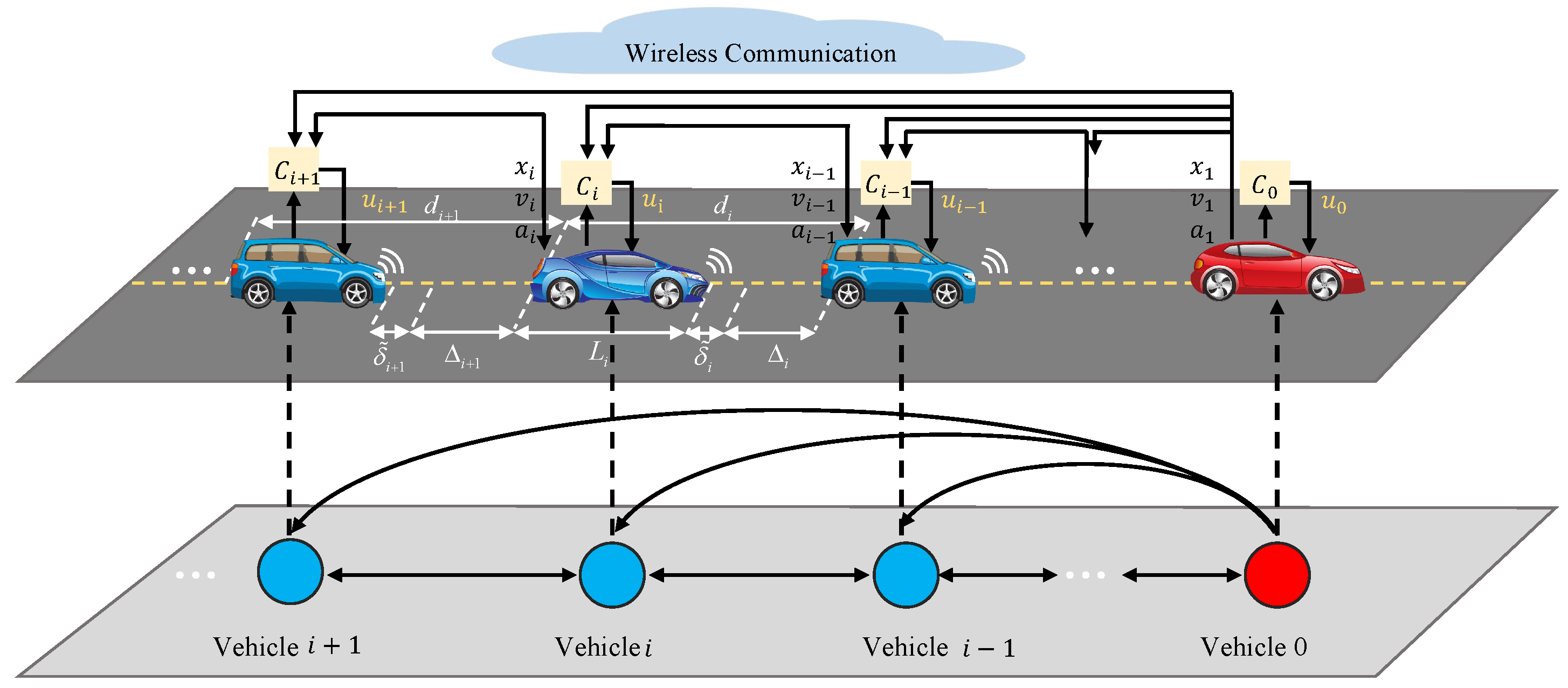
2. Problem Formulation

2.1. Vehicle Dynamics Modeling

Consider a vehicle platoon composed of one leader vehicle and N follower vehicles. The dynamics model of vehicle i $(i\in \{1,2, \dots ,N\left\}\right)$ is considered as [32]

$$\begin{array}{cc}\hfill {\dot{x}}_i\left(t\right)=& v_i\left(t\right)\hfill \\ \hfill {\dot{v}}_i\left(t\right)=& a_i\left(t\right)\hfill \\ \hfill {\dot{a}}_i\left(t\right)=& {\displaystyle \frac{{\eta }_i}{M_i{R}_i{\tau }_i}}sat\left(u_i\left(t\right)\right)-{\displaystyle \frac{1}{M_i{\tau }_i}}\left[{\rho }_a{A}_i{C}_{ai}\right({\displaystyle \frac{1}{2}}{v}_i^2\left(t\right)\hfill \\ \hfill & +{\tau }_i{v}_i\left(t\right)a_i\left(t\right)]-{\displaystyle \frac{1}{{\tau }_i}}{a}_i\left(t\right)+D_i\hfill \end{array}$$

(1)

where $x_i\left(t\right)$ and $a_i\left(t\right)$ denote the position and acceleration of vehicle i, respectively; ${\tau }_i$ represents the engine time constant; ${\eta }_i$ and $M_i$ denote the mechanical efficiency and mass of ith vehicle; $D_i=(1/{\tau }_i){\varpi }_i+{\dot{\varpi }}_i$ with ${\varpi }_i$ representing external disturbances; $R_i$ and $v_i\left(t\right)$ denote the tire radius and velocity of the vehicle i; ${\rho }_a$, $A_i$, and $C_{ai}$ are the density of the air, the area of the frontal cross, and the coefficient of aerodynamic drag, respectively; $u_i\left(t\right)$ is control torque input; and $sat\left(u_i\left(t\right)\right)$ represents the saturation nonlinear function of $u_i\left(t\right)$, and is described as

$$\mathrm{sat}\left(u_i\left(t\right)\right)=\left\{\begin{array}{cc}{u}_{r,imax},\hfill & \mathrm{if}{u}_i\left(t\right)>c_{r,i}\hfill \\ {\mathsf{ȷ}}_{r,i}\left(u_i\left(t\right)\right),\hfill & \mathrm{if}0\le u_i\left(t\right)\le c_{r,i}\hfill \\ {\mathsf{ȷ}}_{l,i}\left(u_i\left(t\right)\right),\hfill & \mathrm{if}{c}_{l,i}\le u_i\left(t\right)<0\hfill \\ u_{l,imin},\hfill & \mathrm{if}{u}_i\left(t\right)<c_{l,i}\hfill \end{array}\right.$$

(2)

where ${\mathsf{ȷ}}_{r,i}\left(u_i\left(t\right)\right)$ and ${\mathsf{ȷ}}_{l,i}\left(u_i\left(t\right)\right)$ represent unknown nonlinear functions; $u_{r,imax}>0$ and $u_{l,imin}<0$ are the bounds of $u_i\left(t\right)$; and $c_{r,i}>0$ and $c_{l,i}<0$ are the saturation amplitudes.

The leader vehicle’s dynamics model is

$$\begin{array}{cc}\hfill {\dot{x}}_0=& v_0\hfill \\ \hfill {\dot{v}}_0=& a_0\hfill \end{array}$$

(3)

where $x_0$ represents the leader’s position; and $a_0$ and $v_0$ are the leader’s acceleration and velocity, respectively. When actuator faults occur, the control input is given by

$$u_{oi}\left(t\right)=(-{\mu }_i+1)sat\left(u_i\left(t\right)\right)+w_i$$

(4)

where ${\mu }_i$ denotes the actuator fault coefficient and satisfies $0<{\mu }_{i1}\le {\mu }_i\le {\mu }_{i2}<1$; ${\mu }_{i1}$ denotes the lower bound of of ${\mu }_i$; ${\mu }_{i2}$ is upper bound of ${\mu }_i$; and $w_i$ denotes the bias faults.

Rewrite (1) as

$$\begin{array}{cc}\hfill {\dot{a}}_i\left(t\right)& ={\displaystyle \frac{{\eta }_i}{M_i{R}_i{\tau }_i}}(1-{\mu }_i)sat\left(u_i\left(t\right)\right)\hfill \\ \hfill & +f_i(v_i,a_i,t)+{\displaystyle \frac{{\eta }_i}{M_i{R}_i{\tau }_i}}{w}_i+D_i\hfill \end{array}$$

(5)

where $f_i(v_i,a_i,t)=-{\displaystyle \frac{1}{M_i{\tau }_i}}\left[{\rho }_a{A}_i{C}_{ai}({\displaystyle \frac{1}{2}}{v}_i^2+{\tau }_i{v}_i{a}_i))\right]-{\displaystyle \frac{1}{{\tau }_i}}{a}_i$ is the nonlinear function.

To address the adverse impacts of $sat\left(u_i\left(t\right)\right)$, we employ the Gaussian Error Function (GEF) to approximate $sat\left(u_i\left(t\right)\right)$. Then, the GEF $\mathsf{ȷ}\left(u_i\left(t\right)\right)$ is constructed as

$$\mathsf{ȷ}\left(u_i\left(t\right)\right)=u_{Mi}\mathcal{G}\left({\displaystyle \frac{\sqrt{\pi }{u}_i}{2u_{Mi}}}\right)$$

(6)

where $u_{Mi}=\left(u_{r,imax}+u_{l,imin}\right)+\left(u_{r,imax}+u_{l,imin}\right)\mathrm{sign}\left(u_i\left(t\right)\right)$, $sign(·)$ is a sign function; $\mathcal{G}\left(j\right)={\displaystyle \frac{2}{\sqrt{\pi }}}{\int }_0^{\mathsf{ȷ}}{e}^{-x^2}dx$.

Then, $sat\left(u_i\left(t\right)\right)$ is defined by the GEF as

$$\mathrm{sat}\left(u_i\left(t\right)\right)=\mathsf{ȷ}\left(u_i\left(t\right)\right)+z_i$$

(7)

where $z_i$ is the GEF approximation error and satisfies $\left|z_i\right|=\left|\mathrm{sat}\left(u_i\left(t\right)\right)-\mathsf{ȷ}\left(u_i\left(t\right)\right)\right|\le {″}_z$ with ${″}_z>0$.

According to the mean-value theorem [33], rewrite (6) as

$$\mathsf{ȷ}\left(u_i\left(t\right)\right)=\mathsf{ȷ}\left(u_{ir}\left(t\right)\right)+h_{{\mu }_i}(u_{ir}\left(t\right)-u_i\left(t\right))$$

(8)

where $h_{{\mu }_i}=e^{-{\left({\displaystyle \frac{\sqrt{\pi }{u}_i^q}{2u_{Mi}}}\right)}^2}$, and $u_i^q=q{u}_i+(1-q)u_{ir}$ with $0<q<1$.

Let $u_{ir}=0$, we have

$$\mathrm{sat}\left(u_i\left(t\right)\right)=h_{{\mu }_i}{u}_i\left(t\right)+z_i$$

(9)

Furthermore, (5) is represented as

$$\begin{array}{c}\hfill {\dot{a}}_i\left(t\right)={\displaystyle \frac{{\eta }_i}{M_i{R}_i{\tau }_i}}(1-{\mu }_i)h_{{\mu }_i}{u}_i\left(t\right)+f_i(v_i,a_i,t)+{\displaystyle \frac{{\eta }_i}{M_i{R}_i{\tau }_i}}{\Gamma }_i\end{array}$$

(10)

where ${\Gamma }_i=((1-{\mu }_i)z_i+w_i)+M_i{R}_i{\tau }_i{D}_i/{\eta }_i$ is the lumped disturbance term.

Assumption 1

([34]). There exists ${\overline{w}}_i >0$, ${\overline{D}}_i> 0$, and ${\overline{\Gamma }}_i >0$ such that $|w_i|\le {\overline{w}}_i$, $|M_i{R}_i{\tau }_i{D}_i/{\eta }_i|\le {\overline{D}}_i$, and $|{\dot{\Gamma }}_i|\le {\overline{\Gamma }}_i$, for $i\in \{1,2,\dots ,N\}$.

2.2. RBFNN

The RBFNN’s structure is depicted in Figure 1. As the RBFNN can approximate any continuous function [32], the nonlinear function is approximated by the RBFNN as

$$f\left(Z\right)=W^T\xi \left(Z\right)+\varsigma$$

(11)

where $Z={[Z_1,Z_2,\dots ,Z_{N_1}]}^T\in {\mathcal{R}}^{N_1}$ denotes the input vector; $W={[W_1,W_2,\dots ,W_{M_1}]}^T\in {\mathcal{R}}^{M_1}$ represents the weight vector, with $M_1$ denoting the number of neurons; $\varsigma$ denotes the approximation error; and $\xi \left(Z\right)={[{\xi }_1\left(Z\right),{\xi }_2\left(Z\right),\dots ,{\xi }_{M_1}\left(Z\right)]}^T$ represents the Gaussian basis function vector, with ${\xi }_k\left(Z\right)$ being expressed by

$${\xi }_k\left(Z\right)=exp\left[-{\displaystyle \frac{{(Z-c_k)}^T(Z-c_k)}{2m_k^2}}\right],k\in \{1,2,\dots ,M_1\}$$

(12)

where $m_k$ represents the width of the Gaussian function; and $c_k$ is the center vector.

According to (11), $f_i(v_i,a_i,t)$ is approximated by the RBFNN as

$$f_i(v_i,a_i,t)={W_i}^{*T}{\xi }_i\left(Z_i\right)+{\zeta }_i$$

(13)

where ${\zeta }_i$ denotes the approximation error satisfying $|{\zeta }_i|\le {\zeta }_i^{*}$, with ${\zeta }_i^{*}>0$; ${W_i}^{*}$ representing the ideal weight vector [35].

2.3. Platoon Control Problem Formulation

The information flow topology of the vehicle platoon is depicted in Figure 2. To remove the dependence of the zero ISEs condition, a novel ESP is designed as

$${\delta }_i\left(t\right)={\tilde{\delta }}_i\left(t\right)-{\Pi }_i$$

(14)

where ${\Pi }_i=({\tilde{\delta }}_i\left(0\right)+[r_i{\tilde{\delta }}_i\left(0\right)+{\tilde{\delta }}_i\left(0\right)]t+0.5[r_i^2{\tilde{\delta }}_i\left(0\right)+2r_i{\dot{\tilde{\delta }}}_i\left(0\right)+{\ddot{\tilde{\delta }}}_i\left(0\right)]t^2)exp(-r_{i}t)$; ${\tilde{\delta }}_i\left(t\right)=d_i-L_i-{\Delta }_i$ with $d_i=x_{i-1}-x_i$; ${\Delta }_i={\phi }_d+{\displaystyle \frac{{\rho }_i(v_i^2-v_0^2)}{2\varphi (1-{\mu }_{i2})}}+{\lambda }_i(1-exp(-{\displaystyle \frac{{\overline{v}}_i}{{\vartheta }_i}}))$ with ${\overline{v}}_i=v_i-v_0$; ${\rho }_i$ and $\varphi$ are the safety coefficient and maximum deceleration, respectively; ${\delta }_i\left(t\right)$ denotes the spacing error; ${\lambda }_i>0$, ${\vartheta }_i>0$ and $r_i>0$; $L_i$ and ${\phi }_d$ represents the vehicle length and predetermined spacing between two adjacent vehicles, respectively.

From (14), we have

$$\begin{array}{cc}\hfill {\delta }_i\left(0\right)& ={\delta }_i\left(t\right){{|}_{t=0}=0,{\dot{\delta }}_i\left(0\right)={\dot{\delta }}_i\left(t\right)|}_{t=0}=0,\hfill \\ \hfill {\ddot{\delta }}_i\left(0\right)& ={\ddot{\delta }}_i{\left(t\right)|}_{t=0}=0\hfill \end{array}$$

(15)

This means that the non-zero ISEs are transformed to zero ISEs by introducing the variable ${\Pi }_i$.

The purpose of this article is to develop a novel nonlinear observer-based distributed adaptive fault-tolerant control strategy for a vehicle platoon to accomplish the following goals:

• Internal stability [36]: Each vehicle keeps the predetermined spacing from the preceding vehicle and achieves velocity synchronization with the leader vehicle.
• String stability [37]: The platoon is regarded to be string stable, if

  $$|{\delta }_N\left(t\right)|\le |{\delta }_{N-1}\left(t\right)|\le \cdots \le |{\delta }_1\left(t\right)|$$

  (16)
• Traffic flow stability [38]: This requires that the gradient $\partial \iota /\phantom{\partial \iota \partial \P }\partial P$ is positive, that is,

  $$\partial \iota /\partial P>0$$

  (17)

  where $\iota$ and P denote the traffic flow rate and traffic density, respectively.

Lemma 1

([39]). If a continuous function $V\left(t\right)\ge 0$, $\forall t\ge 0$ with bounded initial value $V\left(0\right)$ satisfies $\dot{V}\left(t\right)\le -\upsilon V\left(t\right)+\omega$, where $\upsilon >0$ and $\omega >0$, then $V\left(t\right)$ is bounded.

Lemma 2

([40]). For $\forall (y,z)\in {\mathbb{R}}^2$, the inequality holds

$$yz\le {\displaystyle \frac{{\partial }^a}{a}}{\left|y\right|}^a+{\displaystyle \frac{1}{p{\partial }^p}}{\left|z\right|}^p$$

(18)

where $\partial >0$, $a>1$, and $(1-a)(p-1)=1$ with $p>1$.

Lemma 3

([40]). The inequality

$$0\le \left|\nu \right|-\nu tanh\left({\displaystyle \frac{\nu }{ϵ}}\right)\le \varrho ϵ$$

(19)

holds for $\forall ϵ>0$ and $\nu \in \mathbb{R}$, where $\varrho =0.2785$.

3. Nonlinear Observer-Based Distributed Adaptive Fault-Tolerant Control Design

To reduce the adverse effects of external disturbances, a novel nonlinear observer is designed to estimate disturbances without needing to know the upper bounds of the disturbances. A novel adaptive updating mechanism is developed to estimate the unknown time-varying actuator faults. Furthermore, a novel nonlinear observer-based distributed adaptive fault-tolerant strategy based on the developed nonlinear observer, adaptive updating mechanism, RBFNN, and ESP is proposed for the vehicle platoon to accomplish the platoon control objectives.

The sliding mode surface of ith vehicle is constructed as [41]

$${\sigma }_i\left(t\right)=k_d{\dot{\delta }}_i\left(t\right)+k_p{\delta }_i\left(t\right)+{\int }_0^t\left(k_i{\delta }_i\left(\tau \right)+{\psi }_i\left(\tau \right)\right)\mathrm{d}\tau$$

(20)

where $k_d$, $k_p$, and $k_i$ are positive constants; ${\psi }_i\left(t\right)=\hslash (F\left(d_i\left(t\right)\right)-v_i)$, with $F(d_i\left(t\right)$ being given by

$$F\left(d_i\left(t\right)\right)=\left\{\begin{array}{cc}0\hfill & \mathrm{if}{d}_i\le d_s\hfill \\ {\varkappa }_i\left(d_i\left(t\right)\right)\hfill & \mathrm{if}{d}_s<d_i<d_g\hfill \\ v_{max}\hfill & \mathrm{if}{d}_i\ge d_g\hfill \end{array}\right.$$

(21)

where $\hslash >0$, $d_s$ denotes the minimum pre-stopping spacing; $v_{max}$ denotes the vehicle’s maximum velocity; and $d_g$ is the maximum spacing when vehicles maintain $v_{max}$; ${\varkappa }_i\left(d_i\left(t\right)\right)={\displaystyle \frac{v_{max}}{2}}(1-cos\left(\pi {\displaystyle \frac{d_i-d_s}{d_g-d_s}}\right))$.

To ensure the string stability, a couple sliding mode surface is constructed as [6]

$${\overline{\sigma }}_i\left(t\right)=\left\{\begin{array}{c}\phi {\sigma }_i\left(t\right)-{\sigma }_{i+1}\left(t\right),i\in \{1, \dots ,N-1\}\hfill \\ \phi {\sigma }_i\left(t\right),i=N\hfill \end{array}\right.$$

(22)

where $\phi >0$. From (22), we have

$$\begin{array}{c}\hfill \overline{\sigma }\left(t\right)=\Psi \sigma \left(t\right)\end{array}$$

(23)

where $\overline{\sigma }\left(t\right)={\left[{\overline{\sigma }}_1\left(t\right),{\overline{\sigma }}_2\left(t\right),\cdots ,{\overline{\sigma }}_N\left(t\right)\right]}^T,\sigma \left(t\right)={\left[{\sigma }_1\left(t\right),{\sigma }_2\left(t\right),\cdots ,{\sigma }_N\left(t\right)\right]}^T$, and

$$\begin{array}{c}\hfill \Psi =\left[\begin{array}{ccccccccc}\phi & & -1& & \dots & & 0& & 0\\ 0& & \phi & & -1& & \dots & & 0\\ & & & \ddots & & & & \\ 0& & 0& & \dots & & \phi & & -1\\ 0& & 0& & \dots & & 0& & \phi \end{array}\right]\end{array}$$

As $\phi \ne 0$, $\Psi$ is an invertible matrix. According to (22), ${\overline{\sigma }}_i\left(t\right)$ converges to a bounded neighborhood of zero such that ${\sigma }_i$ also converges to a bounded neighborhood of zero [21].

Remark 1.

With the increase in the number of neural network nodes, the number of parameters to be estimated grows rapidly, which places a heavy computational burden on the RBFNN control method [42]. To alleviate this computational burden, we adopt a minimal learning parameter mechanism that makes the number of parameters depend only on the number of vehicles, rather than on the number of neural network nodes [20,38].

3.1. Nonlinear Observer

To estimate the lumped disturbance term, design the nonlinear observer as

$$\begin{array}{c}\hfill \left\{\begin{array}{c}\begin{array}{cc}\hfill {\dot{H}}_i=& {\ell }_i\{a_{i-1}\left(t\right)-a_i\left(t\right)-{\displaystyle \frac{{\rho }_i(a_i^2-a_0^2)}{\varphi (1-{\mu }_i)}}\hfill \\ \hfill & -{\Phi }_i^1({\displaystyle \frac{{\eta }_i}{M_i{R}_i{\tau }_i}}(1-{\mu }_i)h_{{\mu }_i}{u}_i\left(t\right)+f_i(v_i,a_i,t)\hfill \\ \hfill & +{\displaystyle \frac{{\eta }_i{\widehat{\Gamma }}_i}{M_i{R}_i{\tau }_i}})+{\displaystyle \frac{{\lambda }_i{\dot{\overline{v}}}_i^2}{{\vartheta }_i^2}}exp(-{\displaystyle \frac{{\overline{v}}_i}{{\vartheta }_i}})-{\ddot{\Pi }}_i\}-{{\rm Y}}_i\hfill \\ \hfill {\widehat{\Gamma }}_i=& H_i-{\ell }_i{\dot{\delta }}_i\left(t\right)\hfill \end{array}\hfill \end{array}\right.\end{array}$$

(24)

where ${\widehat{\Gamma }}_i$ denotes the estimation of ${\Gamma }_i$; $H_i$ is internal state variable; ${\Phi }_i^1={\displaystyle \frac{{\rho }_i{v}_i}{\varphi (1-{\mu }_{i2})}}+{\displaystyle \frac{{\lambda }_i}{{\vartheta }_i}}exp(-{\displaystyle \frac{{\overline{v}}_i}{{\vartheta }_i}})$; and ${\ell }_i$ represents the observer gain.

An error compensator is proposed as

$${{\rm Y}}_i={\ell }_i{\Phi }_i^1{\displaystyle \frac{{\eta }_i}{M_i{R}_i{\tau }_i}}{\tilde{\Gamma }}_i-{\tilde{\Gamma }}_i$$

(25)

where ${\tilde{\Gamma }}_i={\Gamma }_i-{\widehat{\Gamma }}_i$.

Theorem 1.

Consider the vehicle dynamics (10) under Assumption 1. The designed nonlinear observer (24) and compensator (25) can make ${\tilde{\Gamma }}_i$ converges to $Q_1=\{{\tilde{\Gamma }}_i:{\tilde{\Gamma }}_i\le \sqrt{{\tilde{\Gamma }}_i\left(0\right)+2b_{\gamma }}\}$.

Proof of Theorem 1.

The time derivative of ${\widehat{\Gamma }}_i$ is

$${\dot{\widehat{\Gamma }}}_i={\ell }_i{\Phi }_i^1{\displaystyle \frac{{\eta }_i{\tilde{\Gamma }}_i}{M_i{R}_i{\tau }_i}}-{{\rm Y}}_i$$

(26)

Define the Lyapunov function as $V_{i\Gamma }=(1/2){\tilde{\Gamma }}_i^2$. By differentiating $V_{i\Gamma }$, we have

$$\begin{array}{cc}\hfill {\dot{V}}_{i\Gamma }& ={\tilde{\Gamma }}_i(-{\ell }_i{\Phi }_i^1{\displaystyle \frac{{\eta }_i}{M_i{R}_i{\tau }_i}}{\tilde{\Gamma }}_{i_i}+{{\rm Y}}_i+{\dot{\Gamma }}_i)\hfill \\ \hfill & =-{\ell }_i{\Phi }_i^1{\displaystyle \frac{{\eta }_i}{M_i{R}_i{\tau }_i}}{\tilde{\Gamma }}_i^2+{\tilde{\Gamma }}_i{{\rm Y}}_i+{\tilde{\Gamma }}_i{\dot{\Gamma }}_i\hfill \\ \hfill & =-{\ell }_i{\Phi }_i^1{\displaystyle \frac{{\eta }_i{\tilde{\Gamma }}_i^2}{M_i{R}_i{\tau }_i}}+{\tilde{\Gamma }}_i({\ell }_i{\Phi }_i^1{\displaystyle \frac{{\eta }_i{\tilde{\Gamma }}_i}{M_i{R}_i{\tau }_i}}-{\tilde{\Gamma }}_i)+{\tilde{\Gamma }}_i{\dot{\Gamma }}_i\hfill \\ \hfill & =-{\tilde{\Gamma }}_i{\tilde{\Gamma }}_i+{\tilde{\Gamma }}_i{\dot{\Gamma }}_i\hfill \end{array}$$

(27)

According to Young’s inequality [32], one can obtain

$$\begin{array}{cc}\hfill {\dot{V}}_{i\Gamma }& \le -{\tilde{\Gamma }}_i{\tilde{\Gamma }}_i+{\displaystyle \frac{1}{2}}{\tilde{\Gamma }}_i{\tilde{\Gamma }}_i+{\displaystyle \frac{1}{2}}{\dot{\Gamma }}_i{\dot{\Gamma }}_i\hfill \\ \hfill & \le -{\displaystyle \frac{1}{2}}{\tilde{\Gamma }}_i{\tilde{\Gamma }}_i+{\displaystyle \frac{1}{2}}{\overline{\Gamma }}_i^2\hfill \\ \hfill & \le -{\displaystyle \frac{1}{2}}{\left|{\tilde{\Gamma }}_i\right|}^2+b_{\gamma }\hfill \end{array}$$

(28)

where $b_{\gamma }=(1/2){\overline{\Gamma }}_i^2$ and ${\dot{V}}_{i\Gamma }\le -V_{i\Gamma }+b_{\gamma }$. According to Lemma 1, it can be derived that $V_{i\Gamma }$ is bounded. Therefore, ${\tilde{\Gamma }}_i$ will converge to $Q_1=\{{\tilde{\Gamma }}_i:{\tilde{\Gamma }}_i\le \sqrt{{\tilde{\Gamma }}_i\left(0\right)+2b_{\gamma }}\}$. The proof is concluded. □

3.2. Nonlinear Observer-Based Distributed Adaptive Fault-Tolerant Control Design

${\tilde{\theta }}_i$, ${\tilde{\zeta }}_i$, and ${\tilde{\mu }}_i$ denote estimation errors represented by

$$\begin{array}{cc}\hfill {\tilde{\theta }}_i& ={\theta }_i^{*}-(1-{\mu }_{i2}){\widehat{\theta }}_i\hfill \\ \hfill {\tilde{\zeta }}_i& ={\zeta }_i^{*}-(1-{\mu }_{i2}){\widehat{\zeta }}_i\hfill \\ \hfill {\tilde{\mu }}_i& ={\mu }_i^{*}-{\widehat{\mu }}_i\hfill \end{array}$$

(29)

where ${\widehat{\theta }}_i$, ${\widehat{\zeta }}_i$, and ${\widehat{\mu }}_i$ denote the estimation of ${\theta }_i^{*}$, ${\zeta }_i^{*}$, and ${\mu }_i^{*}$; ${\theta }_i^{*}$ and ${\mu }_i^{*}$ are given by

$$\begin{array}{cc}\hfill {\theta }_i^{*}& =\parallel {W_f}^{*}{\parallel }^2={W_f}^{*T}{W_f}^{*}\hfill \\ \hfill {\mu }_i^{*}& ={\displaystyle \frac{1}{1-{\mu }_{i2}}}\hfill \end{array}$$

(30)

Design the nonlinear observer-based distributed adaptive fault-tolerant controller as

$$\begin{array}{cc}\hfill u_i=& -{\widehat{\Gamma }}_i+{\displaystyle \frac{M_i{R}_i{\tau }_i}{{\eta }_i{h}_{{\mu }_i}}}[{\displaystyle \frac{\kappa {\overline{\sigma }}_i}{\phi k_d{\Phi }_i^1}}+{\displaystyle \frac{\kappa {\widehat{\mu }}_i{\overline{\sigma }}_i}{(1-{\mu }_{i2})\phi k_d{\Phi }_i^1}}\hfill \\ \hfill & +{\widehat{\zeta }}_{i}tanh({\displaystyle \frac{{\overline{\sigma }}_i}{\chi }})+{\displaystyle \frac{{\Lambda }_i^2{\overline{\sigma }}_i}{|{\Lambda }_i{\overline{\sigma }}_i|+b_{oi}}}{\displaystyle \frac{{\Theta }_i}{\phi k_d{\Phi }_i^1}}\hfill \\ \hfill & +{\displaystyle \frac{b_i^2}{2}}{\widehat{\theta }}_i{\xi }_i^T\left(Z_i\right){\xi }_i\left(Z_i\right){\overline{\sigma }}_i]\hfill \end{array}$$

(31)

where $\chi >0$, $b_{oi}>0$, $b_i>0$, and $\kappa >0$; $0<1/(1-{\mu }_{i2})<{\Theta }_i$; ${\Lambda }_i$ is given by

$$\begin{array}{c}\hfill {\Lambda }_i=\left\{\begin{array}{c}\phi k_d(a_{i-1}-a_i-{\displaystyle \frac{{\rho }_i(a_i^2-a_0^2)}{\varphi (1-{\mu }_{i2})}}+{\displaystyle \frac{{\lambda }_i{\dot{\overline{v}}}^2}{{\vartheta }_i^2}}exp\left(-{\displaystyle \frac{{\overline{v}}_i}{{\vartheta }_i}}\right)\hfill \\ -{\ddot{\Pi }}_i)+\phi k_p{\dot{\delta }}_i(t)+\phi k_i{\delta }_i+\phi {\psi }_i\hfill \\ -{\dot{\sigma }}_{i+1},i\in \{1,2,\dots ,N-1\}\hfill \\ \phi k_d(a_{i-1}-a_i-{\displaystyle \frac{{\rho }_i(a_i^2-a_0^2)}{\varphi (1-{\mu }_{i2})}}+{\displaystyle \frac{{\lambda }_i{\dot{\overline{v}}}^2}{{\vartheta }_i^2}}exp\left(-{\displaystyle \frac{{\overline{v}}_i}{{\vartheta }_i}}\right)\hfill \\ -{\ddot{\Pi }}_i)+\phi k_p{\dot{\delta }}_i+\phi k_i{\delta }_i\left(t\right)+\phi {\psi }_i,i=N\hfill \end{array}\right.\end{array}$$

(32)

The adaptive updating mechanism is designed as

$$\begin{array}{cc}\hfill {\dot{\widehat{\theta }}}_i=& {\alpha }_i\phi k_d{\Phi }_i^1{\displaystyle \frac{b_i^2}{2}}{\xi }_i^T{\xi }_i{\overline{\sigma }}_i^2-{\Xi }_{1i}{\widehat{\theta }}_i\hfill \\ \hfill {\dot{\widehat{\zeta }}}_i=& {\beta }_i\phi k_d{\Phi }_i^1{\overline{\sigma }}_i\tanh \left({\displaystyle \frac{{\overline{\sigma }}_i}{\chi }}\right)-{\Xi }_{2i}{\widehat{\zeta }}_i\hfill \\ \hfill {\dot{\widehat{\mu }}}_i=& {\gamma }_i\kappa {\overline{\sigma }}_i^2-{\Xi }_{3i}{\widehat{\mu }}_i\hfill \end{array}$$

(33)

where ${\widehat{\theta }}_i\ge 0$, ${\widehat{\zeta }}_i\ge 0$, ${\widehat{\mu }}_i\ge 0$; ${\alpha }_i>0$, ${\beta }_i>0$, and ${\gamma }_i\ge 0$; ${\Xi }_{1i}$, ${\Xi }_{2i}$, ${\Xi }_{3i}$ are positive constants.

Theorem 2.

Consider the vehicle dynamics (10) under Assumption 1. The designed nonlinear observer (24), adaptive updating mechanism (33), and nonlinear observer-based distributed adaptive fault-tolerant controller (31) can guarantee that ${\delta }_i\left(t\right)$ converges to a bounded neighborhood of zero, while the string stability of entire vehicle platoon can also be ensured when $0<\phi \le 1$.

Proof of Theorem 2.

Define Lyapunov function as

$$\begin{array}{cc}\hfill V& =\sum _{i=1}^N{V}_i^{\sigma }\hfill \\ \hfill V_i^{\sigma }& ={\displaystyle \frac{1}{2}}{\overline{\sigma }}_i^2+{\displaystyle \frac{1}{2(1-{\mu }_{i2}){\alpha }_i}}{\tilde{\theta }}_i^2+{\displaystyle \frac{1}{2(1-{\mu }_{i2}){\beta }_i}}{\tilde{\zeta }}_i^2+{\displaystyle \frac{1}{2{\gamma }_i}}{\tilde{\mu }}_i^2\hfill \end{array}$$

(34)

Differentiating $V_i^{\sigma }$ yields

$${\dot{V}}_i^{\sigma }={\dot{\overline{\sigma }}}_i{\overline{\sigma }}_i-{\displaystyle \frac{1}{{\alpha }_i}}{\tilde{\theta }}_i{\dot{\widehat{\theta }}}_i-{\displaystyle \frac{1}{{\beta }_i}}{\tilde{\zeta }}_i{\dot{\widehat{\zeta }}}_i-{\displaystyle \frac{1}{{\gamma }_i}}{\tilde{\mu }}_i{\dot{\widehat{\mu }}}_i$$

(35)

From (22), the derivative of ${\overline{\sigma }}_i$ is

$$\begin{array}{cc}\hfill {\dot{\overline{\sigma }}}_i=& \left\{\begin{array}{c}\phi (k_d{\ddot{\delta }}_i+k_p{\dot{\delta }}_i+k_i{\delta }_i+{\psi }_i\hfill \\ -{\dot{\sigma }}_{i+1},i\in \{1,2,\cdots ,N-1\}\hfill \\ \phi (k_d{\ddot{\delta }}_i+k_p{\dot{\delta }}_i+k_i{\delta }_i+{\psi }_i),i=N\hfill \end{array}\right.\hfill \\ \hfill =& -\phi k_d{\Phi }_i^1{\dot{a}}_i+{\Lambda }_i,i\in \{1,2,\cdots ,N\}\hfill \end{array}$$

(36)

According to (22) and (36), one has

$$\begin{array}{cc}\hfill {\dot{\overline{\sigma }}}_i{\overline{\sigma }}_i=& \left(-\phi k_d{\Phi }_i^1{\dot{a}}_i+{\Lambda }_i\right){\overline{\sigma }}_i\hfill \\ \hfill =& -\phi k_d{\Phi }_i^1{\overline{\sigma }}_i({\displaystyle \frac{{\eta }_i}{M_i{R}_i{\tau }_i}}(1-{\mu }_i)h_{{\mu }_i}{u}_i+f_i\hfill \\ \hfill & +{\displaystyle \frac{{\eta }_i}{M_i{R}_i{\tau }_i}}{\Gamma }_i)+{\Lambda }_i{\overline{\sigma }}_i\hfill \\ \hfill =& -\phi k_d{\Phi }_i^1{\overline{\sigma }}_i{\displaystyle \frac{{\eta }_i(1-{\mu }_i)h_{{\mu }_i}}{M_i{R}_i{\tau }_i}}{u}_i\hfill \\ \hfill & -\phi k_d{\Phi }_i^1{\overline{\sigma }}_i{W_f}^{*T}{\xi }_i-\phi k_d{\Phi }_i^1{\overline{\sigma }}_i{\zeta }_i\hfill \\ \hfill & -\phi k_d{\Phi }_i^1{\displaystyle \frac{{\eta }_i}{M_i{R}_i{\tau }_i}}{\Gamma }_i{\overline{\sigma }}_i+{\Lambda }_i{\overline{\sigma }}_i\hfill \\ \hfill \le & -\phi k_d{\Phi }_i^1{\overline{\sigma }}_i{\displaystyle \frac{{\eta }_i(1-{\mu }_i)h_{{\mu }_i}}{M_i{R}_i{\tau }_i}}{u}_i-\phi k_d{\Phi }_i^1{\overline{\sigma }}_i{W_f}^{*T}{\xi }_i\hfill \\ \hfill & +\phi k_d{\Phi }_i^1|{\overline{\sigma }}_i|{\zeta }_i^{*}-\phi k_d{\Phi }_i^1{\displaystyle \frac{{\eta }_i}{M_i{R}_i{\tau }_i}}{\Gamma }_i{\overline{\sigma }}_i+\left|{\Lambda }_i{\overline{\sigma }}_i\right|\hfill \end{array}$$

(37)

According to Lemma 2, one has

$$\begin{array}{cc}& -\phi k_d{\Phi }_i^1{\overline{\sigma }}_i{W_f}^{*T}{\xi }_i\le \phi k_d{\Phi }_i^1{\displaystyle \frac{{b_i}^2}{2}}{\overline{\sigma }}_i^2{\theta }_i^{*}{\xi }_i^T{\xi }_i+{\displaystyle \frac{1}{2{b_i}^2}}\phi k_d{\Phi }_i^1\hfill \end{array}$$

(38)

Then, substituting (38) to (37), we have

$$\begin{array}{cc}\hfill {\dot{\overline{\sigma }}}_i{\overline{\sigma }}_i\le & -\phi k_d{\Phi }_i^1{\overline{\sigma }}_i{\displaystyle \frac{{\eta }_i(1-{\mu }_i)h_{{\mu }_i}}{M_i{R}_i{\tau }_i}}{u}_i\hfill \\ \hfill & +\phi k_d{\Phi }_i^1{\displaystyle \frac{{b_i}^2}{2}}{\overline{\sigma }}_i^2{\theta }_i^{*}{\xi }_i^T{\xi }_i+{\displaystyle \frac{1}{2{b_i}^2}}\phi k_d{\Phi }_i^1\hfill \\ \hfill & +\phi k_d{\Phi }_i^1\left|{\overline{\sigma }}_i\right|{\zeta }_i^{*}-\phi k_d{\Phi }_i^1{\displaystyle \frac{{\eta }_i}{M_i{R}_i{\tau }_i}}{\Gamma }_i{\overline{\sigma }}_i\hfill \\ \hfill & +{\Theta }_i(1-{\mu }_{i2})\left|{\Lambda }_i{\overline{\sigma }}_i\right|\hfill \end{array}$$

(39)

From (33), one can obtain that ${\dot{\widehat{\theta }}}_i+{\Xi }_{1i}{\widehat{\theta }}_i\ge 0$ indicating that ${\widehat{\theta }}_i\ge e^{-{\int }_0^t{\Xi }_{1i}\left(\tau \right)d\tau }{\widehat{\theta }}_i\left(0\right)$. Thus, let ${\widehat{\theta }}_i\left(0\right)\ge 0$, ${\widehat{\theta }}_i$ is non-negative. Similarly, ${\widehat{\zeta }}_i$ and ${\widehat{\mu }}_i$ are also non-negative. Then, combing (31) and (39), one has

$$\begin{array}{cc}\hfill -& \phi k_d{\Phi }_i^1{\overline{\sigma }}_i{\displaystyle \frac{{\eta }_i(1-{\mu }_i)h_{{\mu }_i}}{M_i{R}_i{\tau }_i}}{u}_i\hfill \\ \hfill & \le -\kappa (1-{\mu }_i){{\overline{\sigma }}_i}^2-{\displaystyle \frac{\kappa (1-{\mu }_i){\widehat{\mu }}_i{{\overline{\sigma }}_i}^2}{1-{\mu }_{i2}}}\hfill \\ \hfill & -\phi k_d{\Phi }_i^1(1-{\mu }_{i2}){\overline{\sigma }}_i{\widehat{\zeta }}_{i}tanh\left({\displaystyle \frac{{\overline{\sigma }}_i}{\chi }}\right)\hfill \\ \hfill & -{\Theta }_i(1-{\mu }_{i2}){\displaystyle \frac{{\Lambda }_i^2{\overline{\sigma }}_i^2}{|{\Lambda }_i{\overline{\sigma }}_i|+b_{oi}}}+\phi k_d{\Phi }_i^1{\displaystyle \frac{{\eta }_i{h}_{{\mu }_i}(1-{\mu }_i)}{M_i{R}_i{\tau }_i}}{\widehat{\Gamma }}_i{\overline{\sigma }}_i\hfill \\ \hfill & -\phi k_d{\Phi }_i^1(1-{\mu }_{i2}){\displaystyle \frac{b_i^2}{2}}{\widehat{\theta }}_i{\xi }_i^T{\xi }_i{\overline{\sigma }}_i^2\hfill \end{array}$$

(40)

Due to the fact that $-{\displaystyle \frac{{\Lambda }_i^2{\overline{\sigma }}_i^2}{|{\Lambda }_i{\overline{\sigma }}_i|+b_{oi}}}\le -\left|{\Lambda }_i{\overline{\sigma }}_i\right|+b_{oi}$, (40) becomes

$$\begin{array}{cc}\hfill -& \phi k_d{\Phi }_i^1{\overline{\sigma }}_i{\displaystyle \frac{{\eta }_i(1-{\mu }_i)h_{{\mu }_i}}{M_i{R}_i{\tau }_i}}{u}_i\hfill \\ \hfill & \le -\kappa {{\overline{\sigma }}_i}^2+\kappa {\tilde{\mu }}_i{{\overline{\sigma }}_i}^2-\phi k_d{\Phi }_i^1(1-{\mu }_{i2}){\overline{\sigma }}_i{\widehat{\zeta }}_{i}tanh\left({\displaystyle \frac{{\overline{\sigma }}_i}{\chi }}\right)\hfill \\ \hfill & +{\Theta }_i(1-{\mu }_{i2})b_{oi}-{\Theta }_i(1-{\mu }_{i2})\left|{\Lambda }_i{\overline{\sigma }}_i\right|\hfill \\ \hfill & -\phi k_d{\Phi }_i^1(1-{\mu }_{i2}){\displaystyle \frac{b_i^2}{2}}{\widehat{\theta }}_i{\xi }_i^T{\xi }_i{\overline{\sigma }}_i^2\hfill \\ \hfill & +\phi k_d{\Phi }_i^1{\displaystyle \frac{{\eta }_i{h}_{{\mu }_i}(1-{\mu }_i)}{M_i{R}_i{\tau }_i}}\left|{\widehat{\Gamma }}_i{\overline{\sigma }}_i\right|\hfill \end{array}$$

(41)

According to (33), one can obtain

$$\begin{array}{cc}\hfill & -{\displaystyle \frac{1}{{\alpha }_i}}{\tilde{\theta }}_i{\dot{\widehat{\theta }}}_i-{\displaystyle \frac{1}{{\beta }_i}}{\tilde{\zeta }}_i{\dot{\widehat{\zeta }}}_i-{\displaystyle \frac{1}{{\gamma }_i}}{\tilde{\mu }}_i{\dot{\widehat{\mu }}}_i\hfill \\ \hfill =& -\phi k_d{\Phi }_i^1{\displaystyle \frac{b_i^2}{2}}{\tilde{\theta }}_i{\xi }_i^T{\xi }_i{\overline{\sigma }}_i^2-\phi k_d{\Phi }_i^1{\tilde{\zeta }}_i{\overline{\sigma }}_{i}tanh({\displaystyle \frac{{\overline{\sigma }}_i}{\chi }})\hfill \\ \hfill & -\kappa {\tilde{\mu }}_i{\overline{\sigma }}_i^2+{\displaystyle \frac{{\Xi }_{1i}}{{\alpha }_i}}{\tilde{\theta }}_i{\widehat{\theta }}_i+{\displaystyle \frac{{\Xi }_{2i}}{{\beta }_i}}{\tilde{\zeta }}_i{\widehat{\zeta }}_i+{\displaystyle \frac{{\Xi }_{3i}}{{\gamma }_i}}{\tilde{\mu }}_i{\widehat{\mu }}_i\hfill \end{array}$$

(42)

Combining (35), (39), (41) and (42), one has

$$\begin{array}{cc}\hfill V_i^{\overline{\sigma }}\le & -\kappa {{\overline{\sigma }}_i}^2+{\displaystyle \frac{{\Xi }_{1i}}{{\alpha }_i}}{\tilde{\theta }}_i{\widehat{\theta }}_i+{\displaystyle \frac{{\Xi }_{2i}}{{\beta }_i}}{\tilde{\zeta }}_i{\widehat{\zeta }}_i\hfill \\ \hfill & +\phi k_d{\Phi }_i^1{\zeta }^{*}\left|{\overline{\sigma }}_i\right|-\phi k_d{\Phi }_i^1{\zeta }^{*}{\overline{\sigma }}_{i}tanh({\displaystyle \frac{{\overline{\sigma }}_i}{\chi }})+{\displaystyle \frac{1}{2b_i^2}}\phi k_d{\Phi }_i^1\hfill \\ \hfill & +{\Theta }_i(1-{\mu }_{i2})b_{oi}-\phi k_d{\Phi }_i^1{\displaystyle \frac{{\eta }_i}{M_i{R}_i{\tau }_i}}{\tilde{\Gamma }}_i{\overline{\sigma }}_i+{\displaystyle \frac{{\Xi }_{3i}}{{\gamma }_i}}{\tilde{\mu }}_i{\widehat{\mu }}_i\hfill \end{array}$$

(43)

Based on Lemma 2 and (29), we have

$$\begin{array}{cc}\hfill {\displaystyle \frac{{\Xi }_{1i}}{{\alpha }_i}}{\tilde{\theta }}_i{\widehat{\theta }}_i\le & -{\displaystyle \frac{{\Xi }_{1i}}{2(1-{\mu }_{i2}){\alpha }_i}}{\tilde{\theta }}_i^2+{\displaystyle \frac{{\Xi }_{1i}}{2(1-{\mu }_{i2}){\alpha }_i}}{\theta }_i^{*2}\hfill \\ \hfill {\displaystyle \frac{{\Xi }_{2i}}{{\beta }_i}}{\tilde{\zeta }}_i{\widehat{\zeta }}_i\le & -{\displaystyle \frac{{\Xi }_{2i}}{2(1-{\mu }_{i2}){\beta }_i}}{\tilde{\zeta }}_i^2+{\displaystyle \frac{{\Xi }_{2i}}{2(1-{\mu }_{i2}){\beta }_i}}{\zeta }_i^{*2}\hfill \\ \hfill {\displaystyle \frac{{\Xi }_{3i}}{{\gamma }_i}}{\tilde{\mu }}_i{\widehat{\mu }}_i\le & -{\displaystyle \frac{{\Xi }_{3i}}{2{\gamma }_i}}{\tilde{\mu }}_i^2+{\displaystyle \frac{{\Xi }_{3i}}{2{\gamma }_i}}{\mu }_i^{*2}\hfill \end{array}$$

(44)

According to (43) and (44), one can obtain

$$\begin{array}{cc}\hfill V_i^{\overline{\sigma }}\le & -\kappa {{\overline{\sigma }}_i}^2-{\displaystyle \frac{{\Xi }_{1i}}{2(1-{\mu }_{i2}){\alpha }_i}}{\tilde{\theta }}_i^2-{\displaystyle \frac{{\Xi }_{2i}}{2(1-{\mu }_{i2}){\beta }_i}}{\tilde{\zeta }}_i^2\hfill \\ \hfill & -{\displaystyle \frac{{\Xi }_{3i}}{2{\gamma }_i}}{\tilde{\mu }}_i^2+\phi k_d{\Phi }_i^1{\zeta }^{*}\left|{\overline{\sigma }}_i\right|-\phi k_d{\Phi }_i^1{\zeta }^{*}{\overline{\sigma }}_{i}tanh({\displaystyle \frac{{\overline{\sigma }}_i}{\chi }})\hfill \\ \hfill & +{\displaystyle \frac{1}{2b_i^2}}\phi k_d{\Phi }_i^1+{\Theta }_i(1-{\mu }_{i2})b_{oi}-\phi k_d{\Phi }_i^1{\displaystyle \frac{{\eta }_i}{M_i{R}_i{\tau }_i}}{\tilde{\Gamma }}_i{\overline{\sigma }}_i\hfill \\ \hfill & +{\displaystyle \frac{{\Xi }_{1i}}{2(1-{\mu }_{i2}){\alpha }_i}}{\theta }_i^{*2}+{\displaystyle \frac{{\Xi }_{2i}}{2(1-{\mu }_{i2}){\beta }_i}}{\zeta }_i^{*2}+{\displaystyle \frac{{\Xi }_{3i}}{2{\gamma }_i}}{\mu }_i^{*2}\hfill \end{array}$$

(45)

From Lemma 2, one has

$$\begin{array}{cc}\hfill & \phi k_d{\Phi }_i^1{\displaystyle \frac{{\eta }_i}{M_i{R}_i{\tau }_i}}{\tilde{\Gamma }}_i{\overline{\sigma }}_i\le \phi k_d{\Phi }_i^1{\displaystyle \frac{{\eta }_i}{2M_i{R}_i{\tau }_i}}{\tilde{\Gamma }}_i^2+\phi k_d{\Phi }_i^1{\displaystyle \frac{{\eta }_i}{2M_i{R}_i{\tau }_i}}{\overline{\sigma }}_i^2\hfill \end{array}$$

(46)

Combing (45) and (46), we have

$$\begin{array}{cc}\hfill V_i^{\overline{\sigma }}\le & -\kappa {{\overline{\sigma }}_i}^2-{\displaystyle \frac{{\Xi }_{1i}}{2(1-{\mu }_{i2}){\alpha }_i}}{\tilde{\theta }}_i^2-{\displaystyle \frac{{\Xi }_{2i}}{2(1-{\mu }_{i2}){\beta }_i}}{\tilde{\zeta }}_i^2\hfill \\ \hfill & -{\displaystyle \frac{{\Xi }_{3i}}{2{\gamma }_i}}{\tilde{\mu }}_i^2+\phi k_d{\Phi }_i^1{\displaystyle \frac{{\eta }_i}{2M_i{R}_i{\tau }_i}}{\tilde{\Gamma }}_i^2\hfill \\ \hfill & +\phi k_d{\Phi }_i^1{\displaystyle \frac{{\eta }_i}{2M_i{R}_i{\tau }_i}}{\overline{\sigma }}_i^2+\phi k_d{\Phi }_i^1{\zeta }^{*}\left|{\overline{\sigma }}_i\right|\hfill \\ \hfill & -\phi k_d{\Phi }_i^1{\overline{\sigma }}_i{\zeta }^{*}tanh({\displaystyle \frac{{\overline{\sigma }}_i}{\chi }})+{\displaystyle \frac{1}{2b_i^2}}\phi k_d{\Phi }_i^1+{\Theta }_i(1-{\mu }_{i2})b_{oi}\hfill \\ \hfill & +{\displaystyle \frac{{\Xi }_{1i}}{2(1-{\mu }_{i2}){\alpha }_i}}{\theta }_i^{*2}+{\displaystyle \frac{{\Xi }_{2i}}{2(1-{\mu }_{i2}){\beta }_i}}{\zeta }_i^{*2}+{\displaystyle \frac{{\Xi }_{3i}}{2{\gamma }_i}}{\mu }_i^{*2}\hfill \end{array}$$

(47)

Based on Lemma 3 and (28), (47) can be written as

$$\begin{array}{cc}\hfill V_i^{\overline{\sigma }}\le & -B_i{{\overline{\sigma }}_i}^2-{\displaystyle \frac{{\Xi }_{1i}}{2(1-{\mu }_{i2}){\alpha }_i}}{\tilde{\theta }}_i^2-{\displaystyle \frac{{\Xi }_{2i}}{2(1-{\mu }_{i2}){\beta }_i}}{\tilde{\zeta }}_i^2\hfill \\ \hfill & -{\displaystyle \frac{{\Xi }_{3i}}{2{\gamma }_i}}{\tilde{\mu }}_i^2+{\displaystyle \frac{{\Xi }_{3i}}{2{\gamma }_i}}{\mu }_i^{*2}+\phi k_d{\Phi }_i^1{\displaystyle \frac{({\tilde{\Gamma }}_i\left(0\right)+2b_{\gamma }){\eta }_i}{2M_i{R}_i{\tau }_i}}\hfill \\ \hfill & +0.2785{\mu }_i\phi k_d{\Phi }_i^1{\zeta }^{*}+{\displaystyle \frac{1}{2b_i^2}}\phi k_d{\Phi }_i^1+{\Theta }_i(1-{\mu }_{i2})b_{oi}\hfill \\ \hfill & +{\displaystyle \frac{{\Xi }_{1i}}{2(1-{\mu }_{i2}){\alpha }_i}}{\theta }_i^{*2}+{\displaystyle \frac{{\Xi }_{2i}}{2(1-{\mu }_{i2}){\beta }_i}}{\zeta }_i^{*2}\hfill \end{array}$$

(48)

where $B_i=\kappa -\phi k_d{\Phi }_i^1{\eta }_i/2M_i{R}_i{\tau }_i$.

According to (34) and (48), we have

$$V\le -{\wp }_{1}V+{\wp }_2$$

(49)

where

$$\begin{array}{cc}\hfill {\wp }_1=& min\{2B_i,\underset{1\le i<N}{min}{\Xi }_{1i},\underset{1\le i<N}{min}{\Xi }_{2i},\underset{1\le i<N}{min}{\Xi }_{3i}\}\hfill \\ \hfill {\wp }_2=& \sum _{i=1}^n\{0.2785\chi \phi k_d{\Phi }_i^1{\zeta }^{*}+{\displaystyle \frac{1}{2b_i^2}}\phi k_d{\Phi }_i^1+{\Theta }_i(1-{\mu }_{i2})b_{oi}\hfill \\ \hfill & +{\displaystyle \frac{{\Xi }_{1i}}{2(1-{\mu }_{i2}){\alpha }_i}}{\theta }_i^{*2}+{\displaystyle \frac{{\Xi }_{2i}}{2(1-{\mu }_{i2}){\beta }_i}}{\zeta }_i^{*2}+{\displaystyle \frac{{\Xi }_{3i}}{2{\gamma }_i}}{\mu }_i^{*2}\hfill \\ \hfill & +\phi k_d{\Phi }_i^1{\displaystyle \frac{({\tilde{\Gamma }}_i\left(0\right)+2b_{\gamma }){\eta }_i}{2M_i{R}_i{\tau }_i}}\}\hfill \end{array}$$

Based on Lemma 1, one can obtain

$$V\left(t\right)\le \left(V\left(0\right)-{\displaystyle \frac{{\wp }_2}{{\wp }_1}}\right)e^{-{\wp }_{1}t}+{\displaystyle \frac{{\wp }_2}{{\wp }_1}}\le V\left(0\right)+{\displaystyle \frac{{\wp }_2}{{\wp }_1}}$$

(50)

where

$$\begin{array}{cc}\hfill V\left(0\right)=& \sum _{i=1}^N{\displaystyle \frac{1}{2}}{\overline{\sigma }}_i^2\left(0\right)+{\displaystyle \frac{1}{2(1-{\mu }_{i2}){\alpha }_i}}{\tilde{\theta }}_i^2\left(0\right)\hfill \\ \hfill & +{\displaystyle \frac{1}{2(1-{\mu }_{i2}){\beta }_i}}{\tilde{\zeta }}_i^2\left(0\right)+{\displaystyle \frac{1}{2{\gamma }_i}}{\tilde{\mu }}_i^2\left(0\right).\hfill \end{array}$$

According to (50), one has

$$\underset{t\to \infty }{lim}\sum _{i=1}^N{\displaystyle \frac{1}{2}}{\overline{\sigma }}_i^2\le V\left(0\right)+{\displaystyle \frac{{\wp }_2}{{\wp }_1}}$$

(51)

Furthermore, one has

$$\parallel {\overline{\sigma }}_i\parallel \le \sqrt{2(V\left(0\right)+{\displaystyle \frac{{\wp }_2}{{\wp }_1}})}$$

(52)

This indicates that $\parallel {\overline{\sigma }}_i\parallel$ converge to a bounded neighborhood of zero. Then, from (20) and (22), one can deduce that ${\sigma }_i$ and ${\delta }_i$ also approach a bounded neighborhood of zero, which means that the internal stability is ensured.

According to (22), when ${\overline{\sigma }}_i$ converges to a bounded neighborhood of zero, we have

$$\begin{array}{cc}& \phi \left(k_p{\delta }_i\left(t\right)+{\int }_0^t{k}_i{\delta }_i\left(\tau \right)+{\psi }_i\left(\tau \right)d\tau +k_d{\dot{\delta }}_i\left(t\right)\right)\hfill \\ \hfill =& k_p{\delta }_{i+1}\left(t\right)+{\int }_0^t{k}_i{\delta }_{i+1}\left(\tau \right)+{\psi }_{i+1}\left(\tau \right)d\tau +k_d{\dot{\delta }}_{i+1}\left(t\right)\hfill \end{array}$$

(53)

The Laplace transform of (53) is

$$\begin{array}{c}\hfill \begin{array}{cc}& \phi \left(k_p{\delta }_i\left(s\right)+(k_i{\delta }_i\left(s\right)+{\psi }_i\left(s\right))/s+s\left(k_d{\delta }_i\left(s\right)\right)\right)\hfill \\ \hfill =& k_p{\delta }_{i+1}\left(s\right)+(k_i{\delta }_{i+1}\left(s\right)+{\psi }_i\left(s\right))/s+s\left(k_d{\delta }_{i+1}\left(s\right)\right)\hfill \end{array}\end{array}$$

(54)

where ${\delta }_i\left(s\right)$ is Laplace transform of ${\delta }_i\left(t\right)$. The string stability of the platoon is guaranteed if $0<\phi \le 1$. The proof is completed. □

The considered system can reach a stable state in a finite time, and it is reasonable to assume that $v_i=v_0$ for all ith vehicles when the system is stable. Thus, according to (14), ${\Pi }_i$ will be zero at the steady state and the desired inter-vehicle spacing ℵ can be obtained as

$$\aleph =L+{\phi }_d$$

(55)

Then, the steady traffic density is

$$P=1/\phantom{1(L+{\phi }_d)}(L+{\phi }_d)$$

(56)

Since the flow rate $\iota \left(P\right)=P{v}_0$, we have

$$\iota \left(P\right)=P{v}_0={\displaystyle \frac{v_0}{L+{\phi }_d}}$$

(57)

Under the proposed spacing policy, the stability condition $\partial \iota /\phantom{\partial \iota \partial P}\partial P>0$ is satisfied for all traffic densities, which ensures that the traffic flow remains stable [38]. Thus, the stability of the traffic flow is guaranteed.

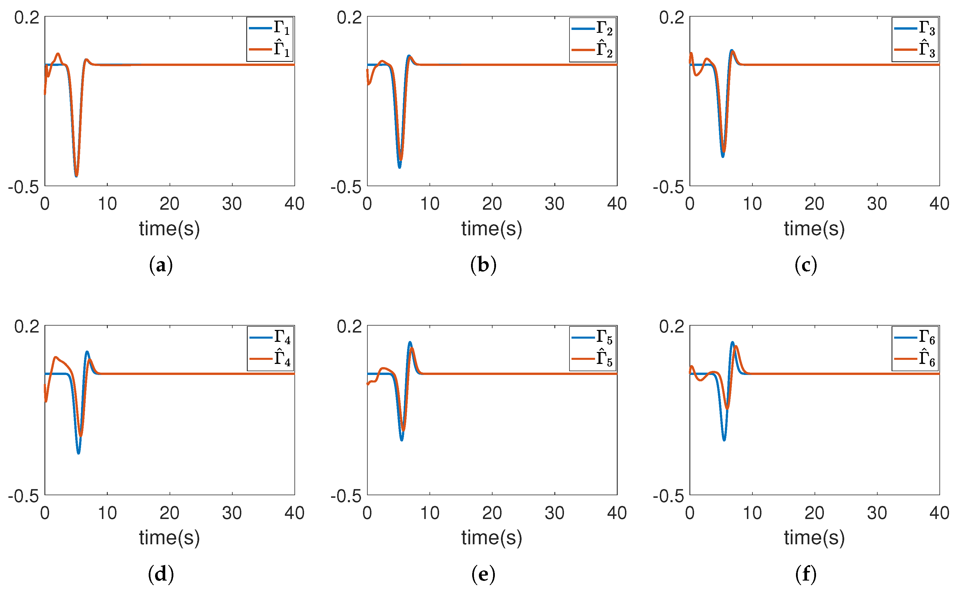
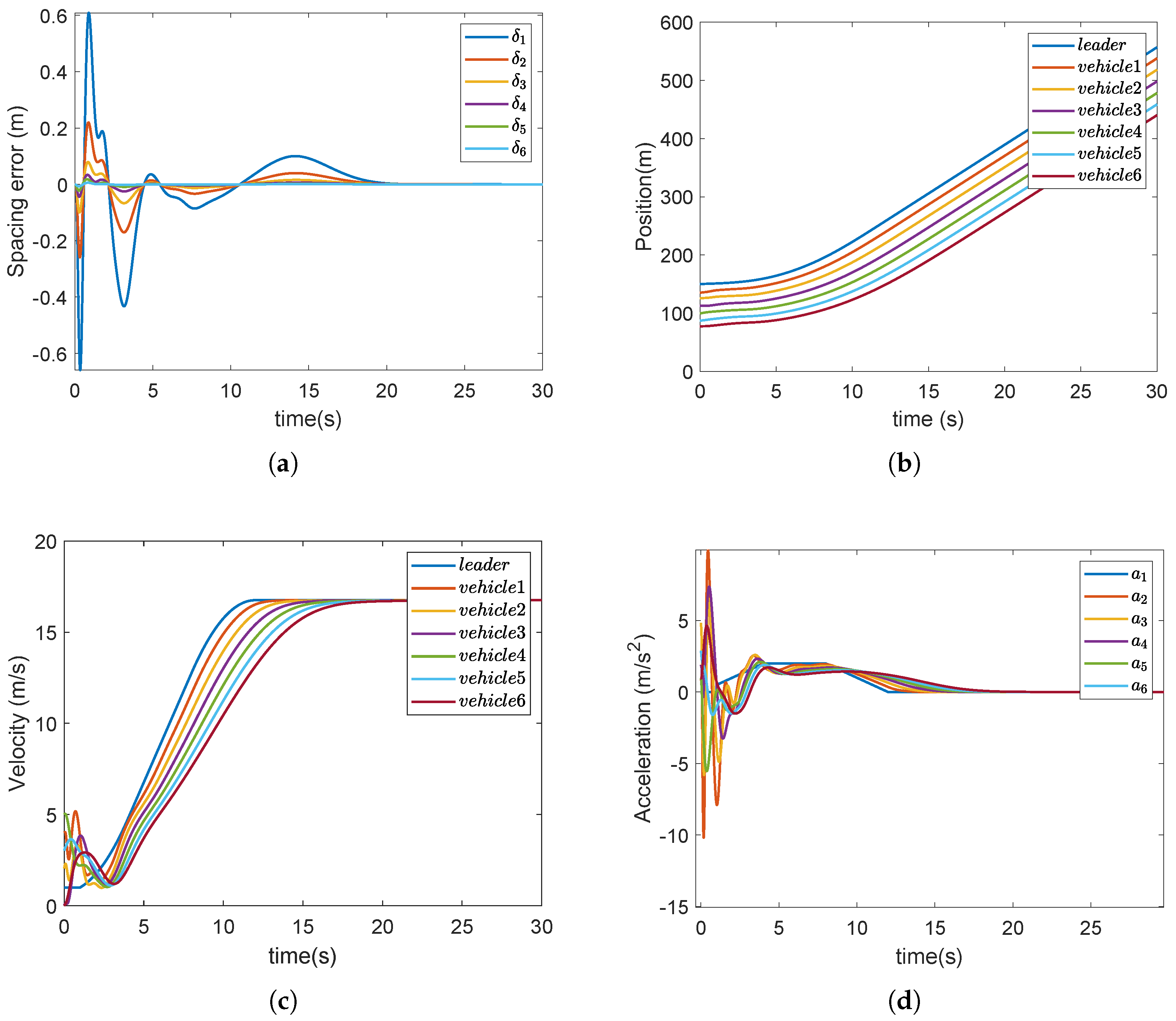
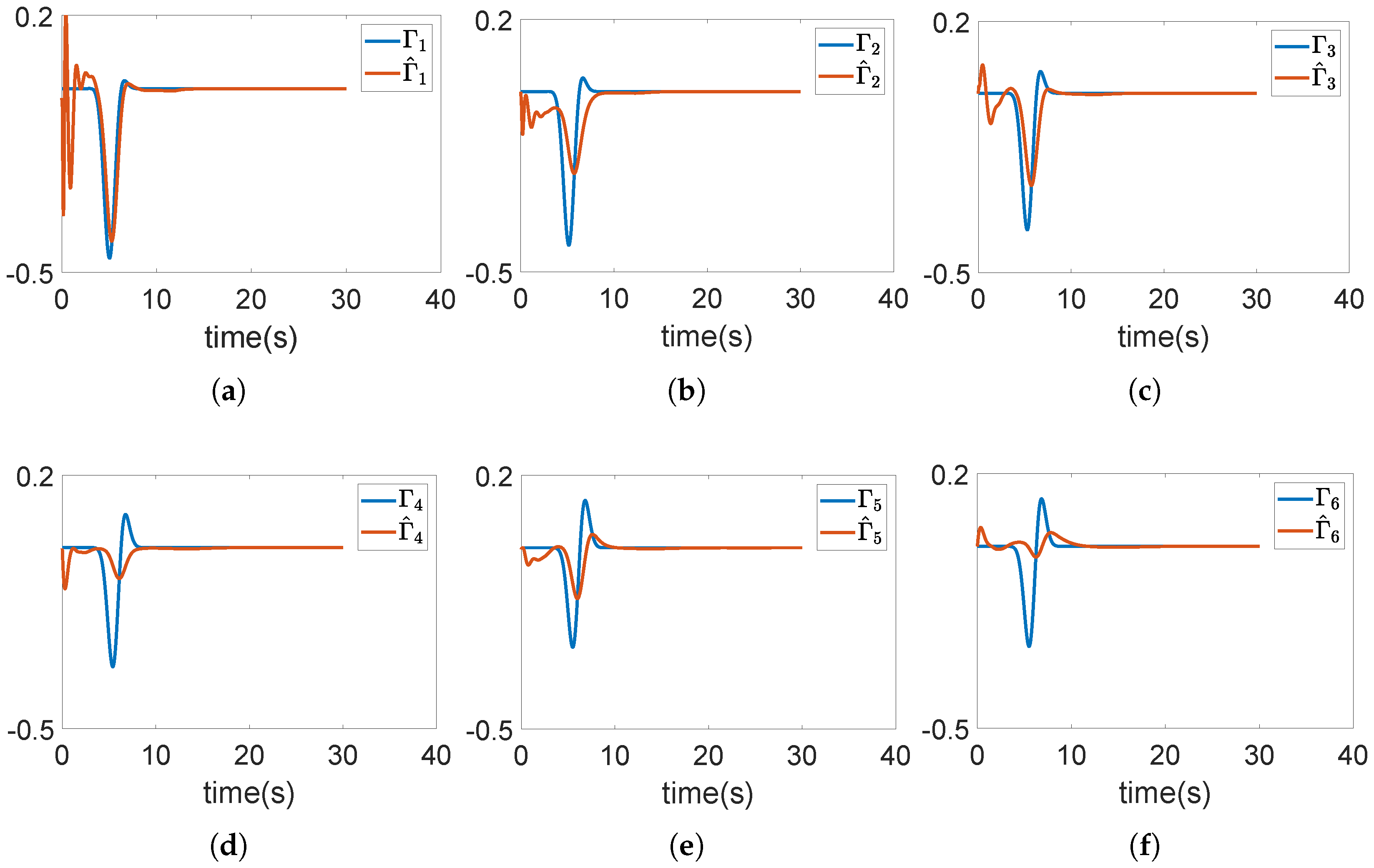
4. Numerical Example

In this section, all numerical examples were conducted using Matlab version 2021b on a laptop made by Lenovo in China, equipped with an Intel Core i7-9700 CPU, 16 GB RAM, and running 64-bit Windows 10. A numerical example is conducted for a vehicle platoon, which comprises one leader vehicle and six follower vehicles, to validate the rightness and effectiveness of the developed controller (31) and adaptive updating mechanism (33). The acceleration profile of leader vehicle is given by

$$\begin{array}{c}\hfill a_0\left(t\right)=\left\{\begin{array}{cc}0.5tm/s^2,\hfill & 1s\le t<4s\hfill \\ 2m/s^2,\hfill & 4s\le t<8s\hfill \\ -0.5t+6m/s^2,\hfill & 8s\le t<12s\hfill \\ 0m/s^2,\hfill & otherwise\hfill \end{array}\right.\end{array}$$

The parameters of the controller and vehicle platoon are ${\rho }_a=1$, $C_{ai}=0.35$, $A_i=2.2$, $g=9.8$, $R_i=0.32$, $M_i=[1500,1600,1550,1650,1500,1400]$, ${\tau }_i=[0.1,0.3,0.2,0.4,0.25,0.4]$, ${\ell }_i=0.1$, ${\rho }_i=0.2$, ${\phi }_d=8$, ${\lambda }_i=0.01$, ${\theta }_i=10$, $\varphi =8$, ${\varpi }_i=0.05sin\left(t\right)$, $k_p=1$, $k_i=2.8$, $k_d=0.15$, $b_i=0.2$, $\chi =0.3$, $b_{oi}=0.8$ [38]. The number of neurons is $M_1=20$. The centers $c_k$ for the input $Z_i\left(t\right)=v_i\left(t\right)$ are evenly spaced in $[-2,5]$, and the widths are $m_k=2(k=1,2,\dots ,20)$. The initial states for all vehicles are $v_i\left(0\right)=[1,4,2,0,5,3,1]$, $a_i\left(0\right)=[0,1,5,2,1,3,1]$. By utilizing the proposed nonlinear observer-based distributed adaptive fault-tolerant controller (31) and adaptive updating mechanism (33), a numerical example is executed on the vehicle dynamics (10) under the information flow topology shown in Figure 2.

The results are obtained as shown in Figure 3. The spacing errors and position profiles are given in Figure 3a,b. As depicted in Figure 3a, the amplitudes of ${\delta }_i$ do not increase along the vehicle platoon, which means that the string stability is achieved. As there are no crossed and overlapped curves in Figure 3b, collisions between adjacent vehicles are avoided. The velocity is given in Figure 3c, which indicates that velocity synchronization is realized among all follower vehicles with the leader. The acceleration profiles are shown in Figure 3d. All followers’ constrained control inputs are given in Figure 3e. From Figure 4, we can see that ${\widehat{\Gamma }}_i$ fluctuates slightly at 5 s, but quickly converges to ${\Gamma }_i$ after 8 s, indicating that the nonlinear observer (24) can effectively estimate ${\Gamma }_i$.

To demonstrate the superior performance of the proposed control strategy, we compared the controller and nonlinear disturbance observer proposed in the paper with the disturbance observer (DO)-based controller and the DO in [19], respectively. All comparisons are based on the vehicle dynamics system described by (1). Figure 5 and Figure 6 present the results of the DO-based controller and the DO.

Table 1. Comparative results of overshoot and ITAE under different controllers.

	Nonlinear Observer-Based Sliding Mode Controller	Disturbance Observer-Based Sliding Mode Controller
Overshoot of ${\delta }_i$	0.0558	0.1317
$ITAE={\sum }_{i=1}^6{\int }_0^{t}t\left|{\delta }_i\left(\tau \right)\right|d\tau$	0.0041	0.0071

and

Table 2. Comparative results of overshoot and ITAE under different DOs.

	Nonlinear Observer	Disturbance Observer
Overshoot of $\tilde{\Gamma }$	0.0915	0.1260
$ITAE={\sum }_{i=1}^6{\int }_0^{t}t\left|\tilde{\Gamma }\left(\tau \right)\right|d\tau$	0.0220	0.0398

provide a quantitative comparison between the two strategies based on the overshoot and the integral of time-weighted absolute error (ITAE) index of ${\delta }_i$ and $\tilde{\Gamma }$.

Figure 5a shows that ${\delta }_i$ decreases along the platoon, indicating that string stability is achieved. From Figure 5b, as the curves do not cross or overlap, it can be seen that collisions between adjacent vehicles are avoided. Figure 5c,d presents the velocity and acceleration curves, which demonstrate that the vehicle platoon achieves velocity synchronization. As shown in Figure 6, ${\widehat{\Gamma }}_i$ converges to ${\Gamma }_i$, indicating that the DO can effectively estimate ${\Gamma }_i$.

According to Table 1, we can observe that compared to the DO-based sliding mode controller, the proposed controller can reduce the overshoot of ${\delta }_i$ by $57.6\%$ and improve the tracking accuracy by $42.2\%$. The quantitative comparison of the performance between the nonlinear observer and the DO is presented in Table 2. According to Table 2, compared to the DO, the nonlinear observer can improve the estimation accuracy of disturbance by $44.7\%$ and reduce the overshoot of $\tilde{\Gamma }$ by $27.3\%$.

5. Conclusions

This work investigates distributed fault-tolerant control for vehicle platoons with actuator faults, saturation, and external disturbances. To mitigate the adverse effects of external disturbances, a novel nonlinear observer is devised to directly estimate external disturbances without the need to know their upper bounds. Considering the situation in which actuator faults may cause partial actuator effectiveness loss, a novel adaptive updating mechanism is developed to estimate this loss. As non-zero ISEs may cause the instability of the vehicle platoon, a novel ESP is developed to reduce their adverse effects. Based on these designs, a nonlinear observer-based distributed adaptive fault-tolerant strategy is developed for the vehicle platoon to address actuator faults, saturation, and external disturbances and ensure the stability of the platoon. A numerical example is used to demonstrate the rightness and effectiveness of the proposed distributed controller. The results show that, using the developed controller, the vehicle platoon objectives can be accomplished, while the disturbances can be effectively estimated by the nonlinear observer. Our future work will focus on the distributed control of vehicle platoons based on reinforcement learning under communication failures.

References

1. Li, X.; Shi, P.; Wang, Y.; Wang, S. Cooperative tracking control of heterogeneous mixed-order multiagent systems with higher-order nonlinear dynamics. IEEE Trans. Cybern. 2020, 52, 5498–5507. [Google Scholar] [CrossRef] [PubMed]
2. Chen, J.; Liang, H.; Li, J.; Lv, Z. Connected automated vehicle platoon control with input saturation and variable time headway strategy. IEEE Trans. Intell. Transp. Syst. 2020, 22, 4929–4940. [Google Scholar] [CrossRef]
3. Qiang, Z.; Dai, L.; Chen, B.; Xia, Y. Distributed model predictive control for heterogeneous vehicle platoon with inter-vehicular spacing constraints. IEEE Trans. Intell. Transp. Syst. 2022, 24, 3339–3351. [Google Scholar] [CrossRef]
4. Hu, M.; Li, C.; Bian, Y.; Zhang, H.; Qin, Z.; Xu, B. Fuel economy-oriented vehicle platoon control using economic model predictive control. IEEE Trans. Intell. Transp. Syst. 2022, 23, 20836–20849. [Google Scholar] [CrossRef]
5. Xu, Z.; Jiao, X. Robust control of connected cruise vehicle platoon with uncertain human driving reaction time. IEEE Trans. Intell. Veh. 2021, 7, 368–376. [Google Scholar] [CrossRef]
6. Kwon, J.; Chwa, D. Adaptive bidirectional platoon control using a coupled sliding mode control method. IEEE Trans. Intell. Transp. Syst. 2014, 15, 2040–2048. [Google Scholar] [CrossRef]
7. Zhu, Y.; Li, Y.; Zhu, H.; Hua, W.; Huang, G.; Yu, S.; Li, S.E.; Gao, X. Joint sliding-mode controller and observer for vehicle platoon subject to disturbance and acceleration failure of neighboring vehicles. IEEE Trans. Intell. Veh. 2022, 8, 2345–2357. [Google Scholar] [CrossRef]
8. Li, X.; Shi, P.; Wang, Y. Distributed cooperative adaptive tracking control for heterogeneous systems with hybrid nonlinear dynamics. Nonlinear Dyn. 2019, 95, 2131–2141. [Google Scholar] [CrossRef]
9. Zheng, Y.; Xu, M.; Wu, S.; Wang, S. Development of connected and automated vehicle platoons with combined spacing policy. IEEE Trans. Intell. Transp. Syst. 2022, 24, 596–614. [Google Scholar] [CrossRef]
10. Mattas, K.; Albano, G.; Donà, R.; He, Y.; Ciuffo, B. On the relationship between traffic hysteresis and string stability of vehicle platoons. Transp. Res. Part B Methodol. 2023, 174, 102785. [Google Scholar] [CrossRef]
11. Zhang, H.; Liu, J.; Wang, Z.; Yan, H.; Zhang, C. Distributed adaptive event-triggered control and stability analysis for vehicular platoon. IEEE Trans. Intell. Transp. Syst. 2020, 22, 1627–1638. [Google Scholar] [CrossRef]
12. Wang, J.; Luo, X.; Wang, L.; Zuo, Z.; Guan, X. Integral sliding mode control using a disturbance observer for vehicle platoons. IEEE Trans. Ind. Electron. 2019, 67, 6639–6648. [Google Scholar] [CrossRef]
13. Zheng, Y.; Zhang, Y.; Qu, X.; Li, S.; Ran, B. Developing platooning systems of connected and automated vehicles with guaranteed stability and robustness against degradation due to communication disruption. Transp. Res. Part Emerg. Technol. 2024, 168, 104768. [Google Scholar] [CrossRef]
14. Kianfar, R.; Falcone, P.; Fredriksson, J. A control matching model predictive control approach to string stable vehicle platooning. Control Eng. Pract. 2015, 45, 163–173. [Google Scholar] [CrossRef]
15. Lin, Y.; Tiwari, A.; Fabien, B.; Devasia, S. Constant-spacing connected platoons with robustness to communication delays. IEEE Trans. Intell. Transp. Syst. 2023, 24, 3370–3382. [Google Scholar] [CrossRef]
16. Chehardoli, H.; Ghasemi, A. Adaptive centralized/decentralized control and identification of 1-D heterogeneous vehicular platoons based on constant time headway policy. IEEE Trans. Intell. Transp. Syst. 2018, 19, 3376–3386. [Google Scholar] [CrossRef]
17. Herman, I.; Knorn, S.; Ahlén, A. Disturbance scaling in bidirectional vehicle platoons with different asymmetry in position and velocity coupling. Automatica 2017, 82, 13–20. [Google Scholar] [CrossRef]
18. Xu, L.; Zhuang, W.; Yin, G.; Bian, C.; Wu, H. Modeling and robust control of heterogeneous vehicle platoons on curved roads subject to disturbances and delays. IEEE Trans. Veh. Technol. 2019, 68, 11551–11564. [Google Scholar] [CrossRef]
19. Wang, Y.; Liu, Y.; Li, X.; Liang, Y. Distributed consensus tracking control based on state and disturbance observations for mixed-order multi-agent mechanical systems. J. Frankl. Inst. 2023, 360, 943–963. [Google Scholar] [CrossRef]
20. Guo, G.; Li, P.; Hao, L.Y. Adaptive fault-tolerant control of platoons with guaranteed traffic flow stability. IEEE Trans. Veh. Technol. 2020, 69, 6916–6927. [Google Scholar] [CrossRef]
21. Wang, J.; Luo, X.; Yan, J.; Guan, X. Distributed integrated sliding mode control for vehicle platoons based on disturbance observer and multi power reaching law. IEEE Trans. Intell. Transp. Syst. 2020, 23, 3366–3376. [Google Scholar] [CrossRef]
22. Boo, J.; Chwa, D. Integral sliding mode control-based robust bidirectional platoon control of vehicles with the unknown acceleration and mismatched disturbance. IEEE Trans. Intell. Transp. Syst. 2023, 24, 10881–10894. [Google Scholar] [CrossRef]
23. Gao, Z.; Zhang, Y.; Guo, G. Prescribed-time control of vehicular platoons based on a disturbance observer. IEEE Trans. Circuits Syst. II Express Briefs 2022, 69, 3789–3793. [Google Scholar] [CrossRef]
24. Afifa, R.; Ali, S.; Pervaiz, M.; Iqbal, J. Adaptive backstepping integral sliding mode control of a mimo separately excited DC motor. Robotics 2023, 12, 105. [Google Scholar] [CrossRef]
25. Wang, Z.; Zhang, B.; Yuan, J. Decentralized adaptive fault tolerant control for a class of interconnected systems with nonlinear multisource disturbances. J. Frankl. Inst. 2018, 355, 4493–4514. [Google Scholar] [CrossRef]
26. Awan, Z.S.; Ali, K.; Iqbal, J.; Mehmood, A. Adaptive backstepping based sensor and actuator fault tolerant control of a manipulator. J. Electr. Eng. Technol. 2019, 14, 2497–2504. [Google Scholar] [CrossRef]
27. Wang, L.; Bian, Y.; Cao, D.; Qin, H.; Hu, M. Hierarchical Safe Control of Heterogeneous Connected Vehicle Systems Using Adaptive Fault-Tolerant Control. IEEE Trans. Veh. Technol. 2024, 73, 14313–14325. [Google Scholar] [CrossRef]
28. An, J.; Cao, L.; Wang, Y.; Khan Jadoon, A.; Wang, S. Adaptive Fault-Tolerant Optimized Platoon Cloud Tracking Control for Heterogeneous Vehicles via Dual Learning Mechanism. IEEE Trans. Autom. Sci. Eng. 2025, 22, 4382–4393. [Google Scholar] [CrossRef]
29. Zhao, Y.; Li, Y. Adaptive fuzzy predefined-time fault-tolerant control for third-order heterogeneous vehicular platoon systems. Int. J. Robust Nonlinear Control 2023, 33, 4422–4437. [Google Scholar] [CrossRef]
30. Yan, S.; Gu, Z.; Park, J.H.; Xie, X.; Sun, W. Distributed cooperative voltage control of networked islanded microgrid via proportional-integral observer. IEEE Trans. Smart Grid 2024, 15, 5981–5991. [Google Scholar] [CrossRef]
31. Yan, S.; Gu, Z.; Park, J.H.; Xie, X. A delay-kernel-dependent approach to saturated control of linear systems with mixed delays. Automatica 2023, 152, 110984. [Google Scholar] [CrossRef]
32. Wu, Z.; Sun, J.; Hong, S. RBFNN-based adaptive event-triggered control for heterogeneous vehicle platoon consensus. IEEE Trans. Intell. Transp. Syst. 2022, 23, 18761–18773. [Google Scholar] [CrossRef]
33. Ren, B.; Ge, S.S.; Su, C.Y.; Lee, T.H. Adaptive neural control for a class of uncertain nonlinear systems in pure-feedback form with hysteresis input. IEEE Trans. Syst. Man, Cybern. Part B (Cybern.) 2008, 39, 431–443. [Google Scholar]
34. Wang, Y.; Shi, P.; Li, X. Event-Triggered Observation-Based Control of Nonlinear Mixed-Order Multiagent Systems Under Input Saturation. IEEE Syst. J. 2024, 18, 1392–1401. [Google Scholar] [CrossRef]
35. Yan, S.; Ding, L.; Cai, Y. Memory-based attack-tolerant TS fuzzy control of networked artificial pancreas system subject to false data injection attacks. Fuzzy Sets Syst. 2025, 518, 109486. [Google Scholar] [CrossRef]
36. Feng, S.; Zhang, Y.; Li, S.E.; Cao, Z.; Liu, H.X.; Li, L. String stability for vehicular platoon control: Definitions and analysis methods. Annu. Rev. Control 2019, 47, 81–97. [Google Scholar] [CrossRef]
37. Besselink, B.; Johansson, K.H. String stability and a delay-based spacing policy for vehicle platoons subject to disturbances. IEEE Trans. Autom. Control 2017, 62, 4376–4391. [Google Scholar] [CrossRef]
38. Guo, G.; Li, P.; Hao, L.Y. A new quadratic spacing policy and adaptive fault-tolerant platooning with actuator saturation. IEEE Trans. Intell. Transp. Syst. 2020, 23, 1200–1212. [Google Scholar] [CrossRef]
39. Guo, X.; Wang, J.; Liao, F.; Teo, R.S.H. CNN-based distributed adaptive control for vehicle-following platoon with input saturation. IEEE Trans. Intell. Transp. Syst. 2017, 19, 3121–3132. [Google Scholar] [CrossRef]
40. Pan, C.; Chen, Y.; Liu, Y.; Ali, I.; He, W. Distributed finite-time fault-tolerant control for heterogeneous vehicular platoon with saturation. IEEE Trans. Intell. Transp. Syst. 2022, 23, 21259–21273. [Google Scholar] [CrossRef]
41. Jin, I.G.; Orosz, G. Optimal control of connected vehicle systems with communication delay and driver reaction time. IEEE Trans. Intell. Transp. Syst. 2016, 18, 2056–2070. [Google Scholar] [CrossRef]
42. Chen, M.; Tao, G. Adaptive Fault-Tolerant Control of Uncertain Nonlinear Large-Scale Systems With Unknown Dead Zone. IEEE Trans. Cybern. 2016, 46, 1851–1862. [Google Scholar] [CrossRef] [PubMed]
Figure 1. RBFNN structure.
Electronics 14 02879 g001
Figure 2. Information flow topology of vehicle platoon.
Electronics 14 02879 g002
Figure 3. The results of the proposed nonlinear observer-based distributed adaptive fault-tolerant controller. (a) Spacing error δ i . (b) Position of ith vehicle. (c) Velocity of ith vehicle. (d) Acceleration of ith vehicle. (e) Control inputs u i .
Electronics 14 02879 g003
Figure 4. The estimation results of the proposed nonlinear observer. (a) The estimation result of Γ 1 . (b) The estimation result of Γ 2 . (c) The estimation result of Γ 3 . (d) The estimation result of Γ 4 . (e) The estimation result of Γ 5 . (f) The estimation result of Γ 6 .
Electronics 14 02879 g004
Figure 5. The results by using the DO-based controller in [19]. (a) Spacing error δ i . (b) Position of ith vehicle. (c) Velocity of ith vehicle. (d) Acceleration of ith vehicle.
Electronics 14 02879 g005
Figure 6. The estimation results by using the disturbance observer in [19]. (a) The estimation result of Γ 1 . (b) The estimation result of Γ 2 . (c) The estimation result of Γ 3 . (d) The estimation result of Γ 4 . (e) The estimation result of Γ 5 . (f) The estimation result of Γ 6 .
Electronics 14 02879 g006