Transient Stability Assessment of Power Systems Based on Temporal Feature Selection and LSTM-Transformer Variational Fusion

Abstract

To address the challenges brought by the high penetration of renewable energy in power systems, such as multi-scale dynamic interactions, high feature dimensionality, and limited model generalization, this paper proposes a transient stability assessment (TSA) method that combines temporal feature selection with deep learning-based modeling. First, a two-stage feature selection strategy is designed using the inter-class Mahalanobis distance and Spearman rank correlation. This helps extract highly discriminative and low-redundancy features from wide-area measurement system (WAMS) time-series data. Then, a parallel LSTM-Transformer architecture is constructed to capture both short-term local fluctuations and long-term global dependencies. A variational inference mechanism based on a Gaussian mixture model (GMM) is introduced to enable dynamic representations fusion and uncertainty modeling. A composite loss function combining improved focal loss and Kullback–Leibler (KL) divergence regularization is designed to enhance model robustness and training stability under complex disturbances. The proposed method is validated on a modified IEEE 39-bus system. Results show that it outperforms existing models in accuracy, robustness, interpretability, and other aspects. This provides an effective solution for TSA in power systems with high renewable energy integration.

1. Introduction

With a large number of renewable energy sources being connected to the power grid through power electronic devices, the dynamic behavior of power systems has evolved from slow dynamics dominated by synchronous generators to fast responses with multi-timescale coupling. This transition increases system nonlinearity and uncertainty, thereby elevating the risk of transient instability [1,2]. In this context, developing efficient and accurate TSA methods is crucial for the secure operation of modern power systems.

Traditional TSA methods include time-domain simulation and the energy function method [2]. Although the former can accurately capture system dynamics, it suffers from high computational complexity, whereas the latter is highly sensitive to high-order nonlinearities in systems with high renewable energy penetration. As a result, both methods are inadequate, especially for online assessment under multi-disturbance and multi-scenario conditions [3]. In recent years, data-driven methods have emerged as a promising alternative by directly mapping WAMS data to system stability status. 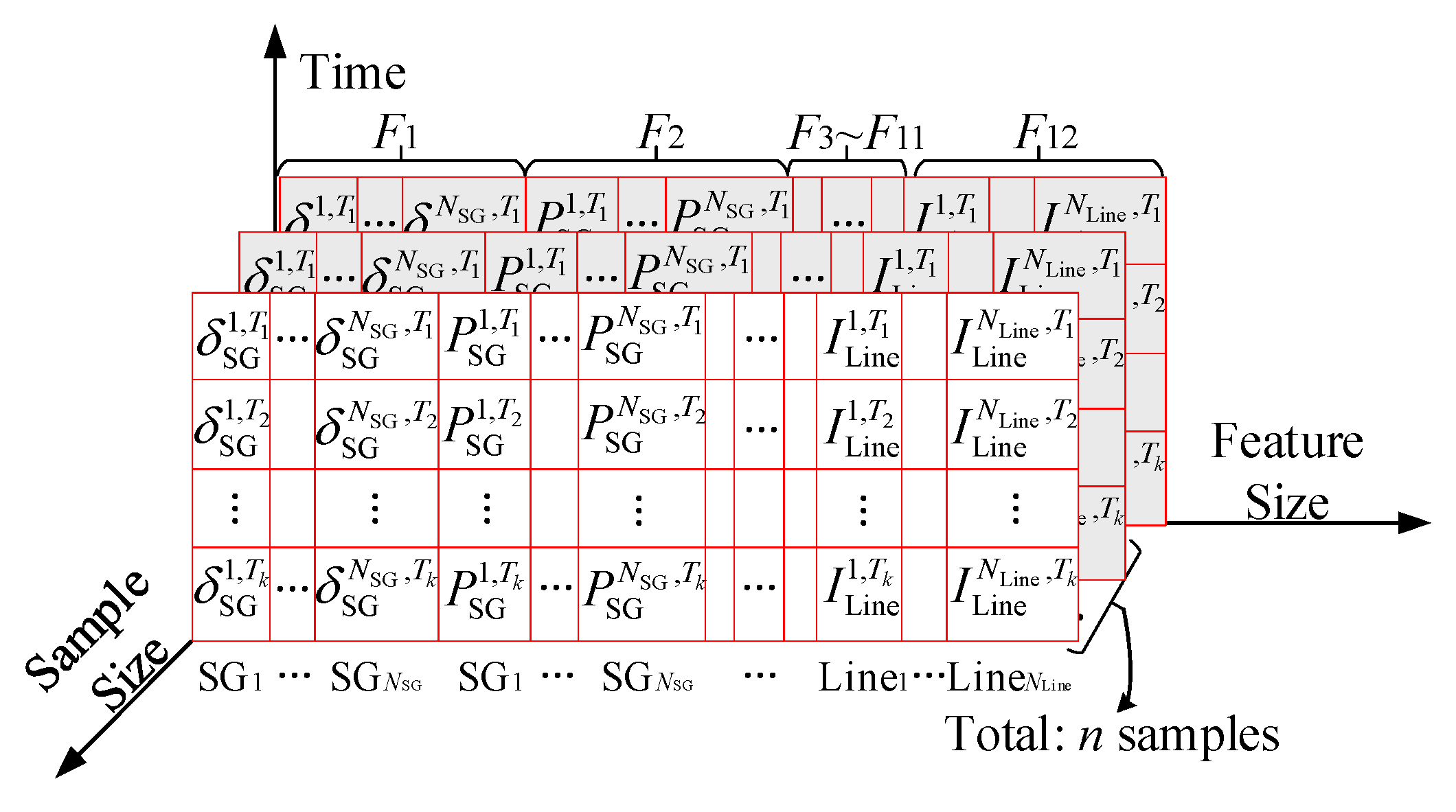This approach eliminates the reliance on complex physical models and significantly improves assessment efficiency [4]. A typical data-driven framework consists of three core components: dataset construction and preprocessing, stability-oriented representation learning, and classifier design and optimization.

In the dataset construction and preprocessing component, key steps include disturbance window extraction, data normalization, and the elimination of redundant or poorly discriminative features. These steps aim to improve data quality and reduce input dimensionality. Here, “features” refers broadly to the input data, while “representations” denotes the model-extracted temporal embeddings used for stability evaluation. Most existing studies construct datasets using bus voltage, frequency, and other measurements from WAMSs. However, due to strong correlations among variables and variations in the responses of the same type of measurements (e.g., voltage) across different buses, directly using all features often introduces redundancy, increases computational overhead, and leads to overfitting. To improve input effectiveness, previous studies have employed Pearson correlation [5], gradient boosting-based dimensionality reduction [6], and distance-based methods such as Relief-F [7] and the Fisher Score [8]. Some methods rely heavily on model structures and lack adaptability. Others are more general but focus on static features and cannot capture the dynamic dependencies in disturbance responses. High-quality inputs are essential for accurate and robust stability state representation. However, existing methods often overlook the temporal response behavior at the feature group level, leading to a mismatch with actual operating conditions and limiting model robustness and generalization [9].

The stability-oriented representation learning component aims to reveal multivariate temporal dependencies and discriminative patterns during fault responses, forming dynamic representations that indicate system stability. Conventional machine learning methods, such as support vector machines [10] and decision trees [11], rely on expert-designed static features. These approaches struggle to capture the nonlinear dynamic behaviors of multivariate systems under high renewable penetration and often suffer from poor generalization [4]. In contrast, deep learning enables end-to-end modeling, allowing systems to learn dynamic evolution patterns directly from raw data, thereby avoiding the subjectivity of manual feature engineering. 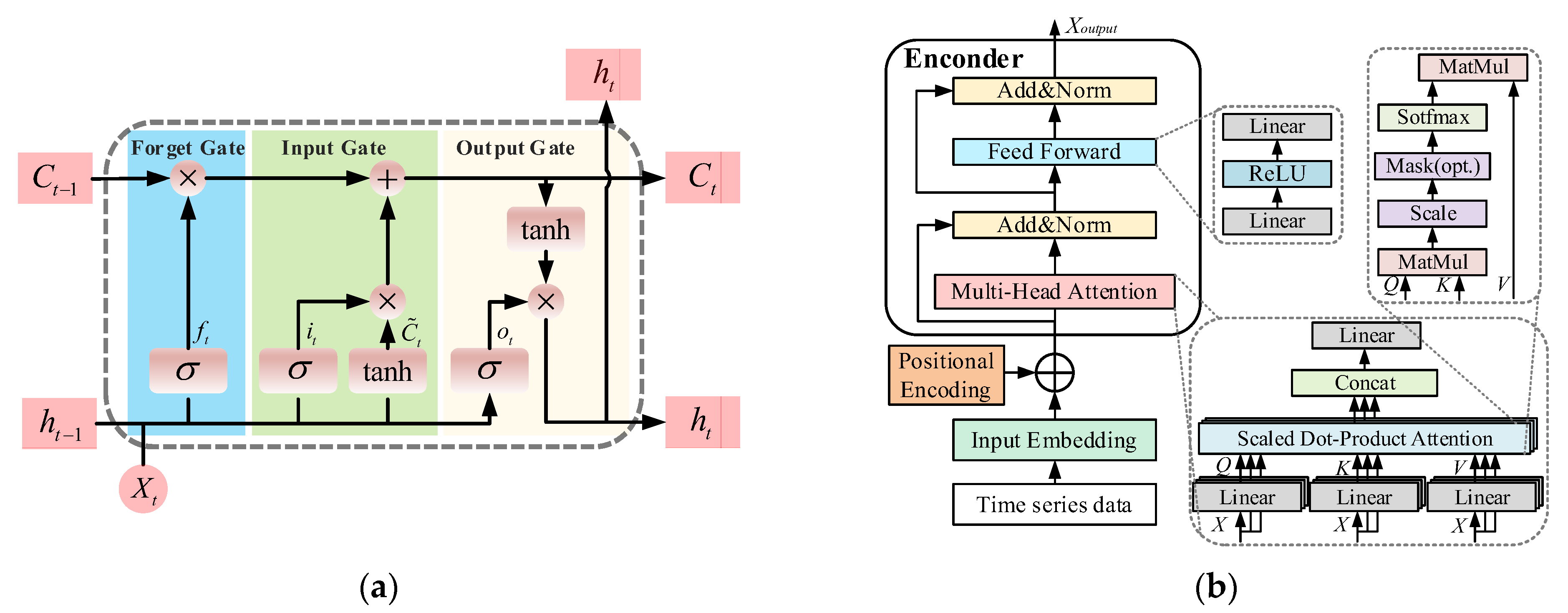Common deep learning models applied to TSA include deep belief networks (DBN) [12], convolutional neural networks (CNNs) [13], and long short-term memory (LSTM) networks [14], among others. LSTM excels at capturing short-term temporal dependencies as it is sensitive to local fluctuations in the early stages of a fault and can effectively extract sudden changes in individual measurements [15]. In contrast, the Transformer, with its self-attention mechanism, is well-suited for modeling long-term dependencies, enabling it to capture system-wide responses throughout the entire fault process [1,16]. However, in modern power systems, the fast control responses of renewable sources coexist with the slow inertial regulation of conventional generators, resulting in multi-timescale dynamics that couple abrupt and gradual changes [17].

Meanwhile, diverse control strategies and varying fault responses [18] further increase the complexity of dynamic representation learning. Single-architecture deep learning models struggle to capture such multi-scale and multi-pattern behaviors, leading to limited perception and inadequate modeling capacity [19]. To enhance the perception and discrimination of multi-scale representations, various hybrid network structures have been proposed. Representative efforts include CNN-LSTM frameworks for joint spatial–temporal representation extraction [20], and multi-level assessment models integrating DBN, CNNs, and LSTM to quantify stability margins [21]. Nonetheless, most methods combine learned representations from different networks through static concatenation or simple weighting, lacking adaptive integration of multi-source representations. This often leads to information loss and error buildup, increasing the risk of misclassification under complex disturbances.

The classifier design and optimization component mainly involves two aspects: the selection of classifier structures and the design of loss functions. The former typically employs perceptions or fully connected networks for stability classification, offering good performance. The latter involves designing loss functions to help the model distinguish between stable and unstable cases more effectively. Cross-entropy loss is widely used but struggles with class imbalance and ambiguous decision boundaries. To address these issues, some studies adopt focal loss to assign greater weight to uncertain or hard-to-distinguish samples [13,22]. To enhance the stability identification performance and generalization capability of TSA models, the loss function should be specifically designed based on both power system instability characteristics and the model architecture.

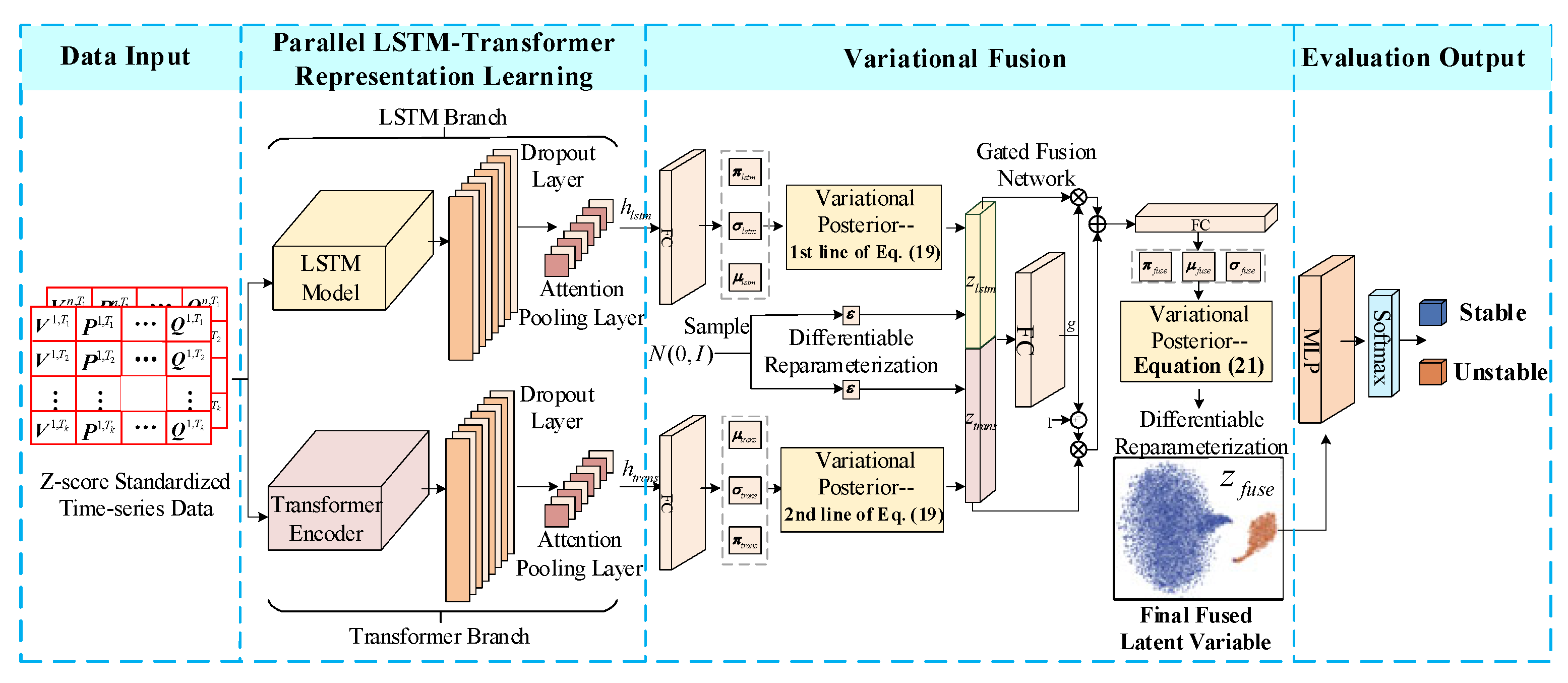
To address the above issues, this paper proposes a TSA method combining temporal feature selection with the variational fusion of representations extracted by LSTM and a Transformer. This design facilitates efficient representation learning across multiple temporal scales, particularly for power systems with high renewable energy penetration. The main contributions of this paper are as follows:

(1)

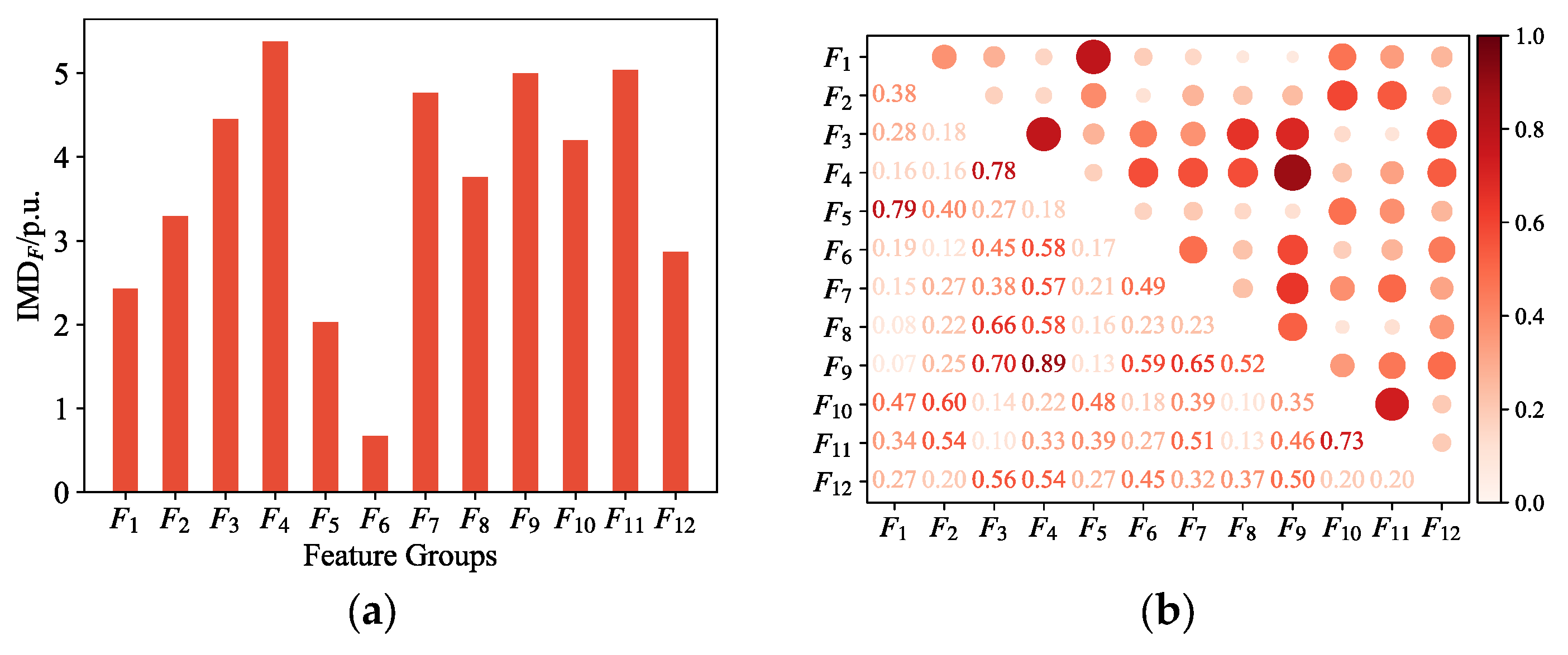
A two-stage temporal feature selection method is proposed. It first evaluates the discriminative ability of feature groups via inter-class Mahalanobis distance, then removes redundancy using Spearman correlation coefficients and selects key features through an incremental feature subset strategy.

(2)

A parallel LSTM-Transformer architecture is developed to extract heterogeneous representations at different timescales. Variational inference based on a GMM is applied separately to each branch for probabilistic modeling. A gated fusion network is further introduced to unify latent representations, forming a variational fusion mechanism capable of cross-scale perception.

(3)

A composite loss function is designed by combining an improved focal loss with a KL divergence regularization term. It addresses class imbalance while guiding the model to learn latent representations with enhanced discriminability and distributional stability.

From an engineering perspective, the proposed method supports fast and reliable online stability assessment in power systems with high renewable penetration. The temporal feature selection strategy reduces input dimensionality, which, in turn, lowers the reliance on system-wide measurements and simplifies deployment and data requirements. It enables millisecond-level evaluation through a single forward pass, and the model is designed to be robust against noise and missing data, making it suitable for practical protection and control applications.

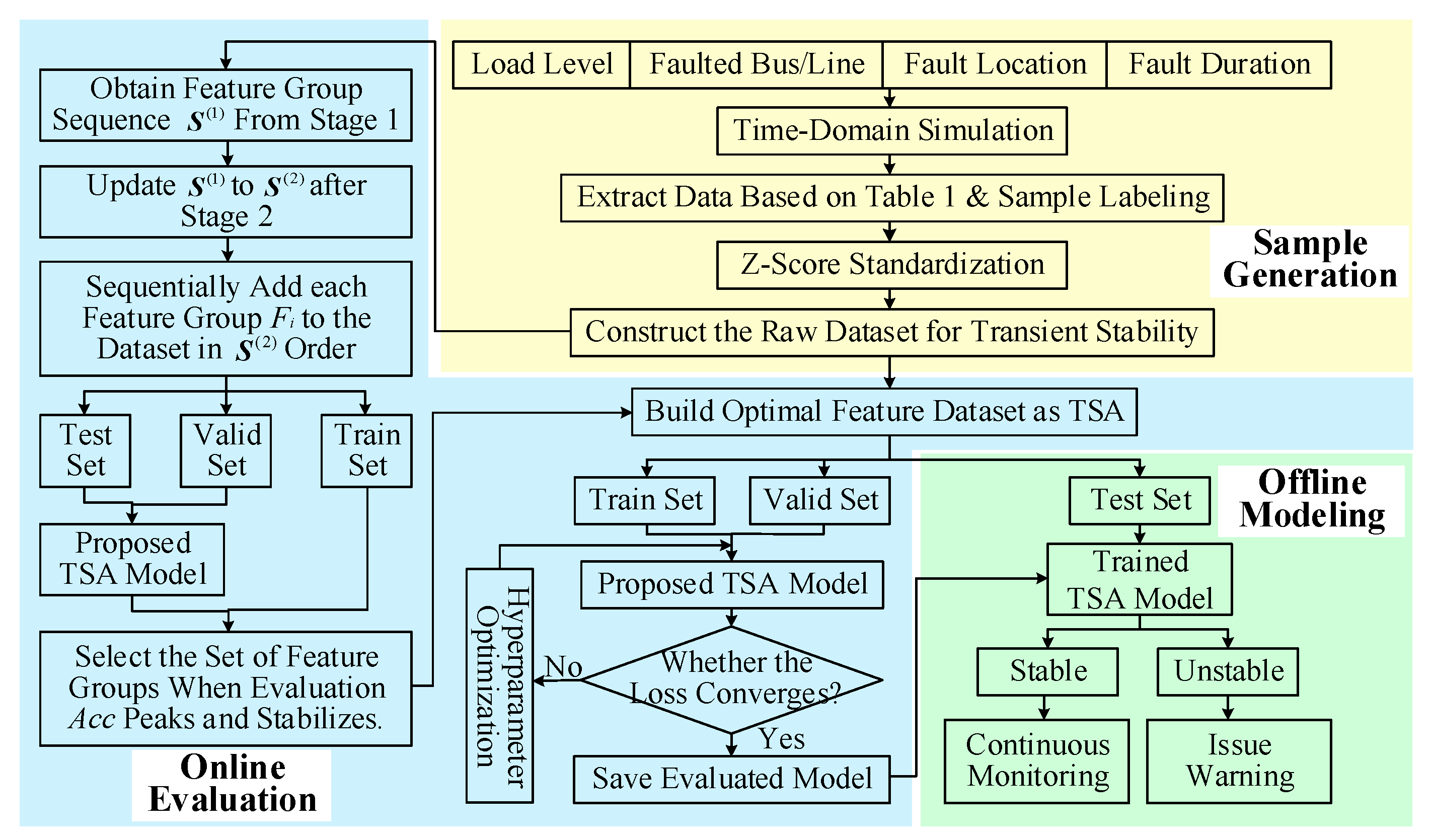
The rest of the paper is organized as follows: Section 2 outlines the data-driven TSA principle and the construction of the input feature space. A two-stage temporal feature selection method is proposed in Section 3. Section 4 introduces the LSTM-Transformer variational fusion model, along with the design of a composite loss function. The overall implementation process is detailed in Section 5. Section 6 validates the effectiveness and superiority of the proposed method through case studies. Finally, Section 7 concludes the paper and outlines future research directions.

2. Modeling Framework for Transient Stability Assessment Based on Temporal Data

2.1. Principles of Data-Driven Transient Stability Assessment

The transient process of power systems involves all the dynamic responses of components in the grid, causing changes in electrical quantities at all nodes and branches. Data-driven TSA is based on the relationship between temporal variations and system stability, using data-driven models to link input temporal features with stability classification outputs. When employing deep learning algorithms for TSA, the input data of sample i can be represented as a temporal feature matrix ${\mathit{X}}_i\in {ℝ}^{k\times m}$, where k is the number of time steps and m is the feature dimension. The corresponding output label is a binary classification indicating stability or instability, defined as follows:

$$y_i=\left\{\begin{array}{l}0, \mathrm{Stable}\\ 1, \mathrm{Unstable}\end{array}\right.$$

(1)

In data-driven TSA, a classification model is trained to learn the mapping between input data X and labels y. If an appropriate mapping is found, the model can achieve reliable assessment performance. The sample labels indicating the stability status are determined by the transient stability index (TSI) based on the rotor angle after fault clearance [16], which is defined as follows:

$$C_{\mathrm{TSI}}={\displaystyle \frac{360-\left|\Delta {\delta }_{\max }\right|}{360+\left|\Delta {\delta }_{\max }\right|}}$$

(2)

where Δδ_max is the maximum relative rotor angle difference in degree between any two synchronous machines during the simulation period. A sample is considered stable if C_TSI > 0 and unstable otherwise.

2.2. Construction of the Input Feature Space

Data-driven TSA relies on large numbers of historical data for training; the more comprehensive the data, the better the model can represent system dynamics [8]. Accordingly, this study conducts extensive simulations to construct a feature set comprising 12 types of power system variables, as listed in

Table 1. Original input features for TSA.

Feature ID	Feature Description	Feature ID	Feature Description
F1	Rotor Angle of SG (δSG)	F7	Active Power of DFIG (PDFIG)
F2	Active Power of SG (PSG)	F8	Reactive Power of DFIG (QDFIG)
F3	Reactive Power of SG (QSG)	F9	Active Power of PV (PPV)
F4	Bus Voltage Magnitude (VBus)	F10	Active Power of Load (PLoad)
F5	Bus Voltage Angle (δBus)	F11	Reactive Power of Load (QLoad)
F6	Bus Frequency (fBus)	F12	Line Current (ILine)

. As photovoltaic stations mainly generate active power, their relatively small reactive output is excluded from modeling. The temporal features listed in Table 1 are unfiltered original inputs, and their high dimensional redundancy will be addressed through a subsequent feature selection process.

The number of temporal features under each feature type in Table 1 (e.g., voltage magnitude or generator active power) varies with system scale, as each type corresponds to multiple nodes or devices in the system. During simulation, k time steps of data are collected before and after fault clearance. Each sample is organized as a two-dimensional matrix (time steps × features), and all samples are stacked into a 3D tensor of size n × k × m, where n is the number of samples, as shown in Figure 1. To eliminate scale differences, all data are z-score standardized before training [23].

3. Two-Stage Temporal Feature Selection

3.1. Stage One: Ranking Feature Groups by Discriminative Power via Inter-Class Mahalanobis Distance

Mahalanobis distance (MD) is commonly used in unsupervised pattern recognition to measure how far a sample deviates from a class center [24]. However, in feature selection for power system TSA, the key requirement is to evaluate how well features distinguish between stable and unstable states, which is inherently a supervised task. Therefore, we modify the MD by introducing the inter-class Mahalanobis distance (IMD), which quantifies the discriminative ability of each temporal feature f_i between classes. Importantly, the original temporal dimension is preserved to avoid loss of dynamic information due to feature compression. The mathematical definition is as follows:

$${\mathrm{IMD}}_{f_i}=\sqrt{{({\mathit{\mu }}_{f_i}^{(0)}-{\mathit{\mu }}_{f_i}^{(1)})}^T{\left({\mathit{M}}_{f_i}^{reg}\right)}^{-1}({\mathit{\mu }}_{f_i}^{(0)}-{\mathit{\mu }}_{f_i}^{(1)})}$$

(3)

where ${\mathit{\mu }}_{f_i}^{(0)},{\mathit{\mu }}_{f_i}^{(1)}$ denote the temporal mean vectors of feature f_i under the stable (y = 0) and unstable (y = 1) classes, respectively, and ${\mathit{M}}_{f_i}^{reg}$ is the regularized covariance matrix computed from the combined samples of both classes. Conventional sample covariance matrices are prone to ill-conditioning or singularity in high-dimensional, small-sample scenarios, which undermines the stability of IMD computation. Therefore, the Ledoit–Wolf shrinkage estimator with trace normalization is employed, formulated as follows:

$${\mathit{M}}_{f_i}^{reg}=\rho \mathit{I}+(1-\rho ){\mathit{M}}_{f_i}+\epsilon \cdot {\displaystyle \frac{\mathrm{Tr}\left(\rho \mathit{I}+(1-\rho ){\mathit{M}}_{f_i}\right)}{k}}\cdot \mathit{I}$$

(4)

where $\rho$ is the adaptive shrinkage coefficient, I denotes the identity matrix, ${\mathit{M}}_{f_i}$ is the standard empirical covariance matrix, Tr(·) denotes the trace operator (i.e., the sum of eigenvalues), k is the dimension of ${\mathit{M}}_{f_i}$, and ε = 10⁻⁷.

For each physically related feature group F, the average IMD of all temporal features within the group is further defined as the overall discriminative power of the group.

$${\mathrm{IMD}}_F={\displaystyle \frac{1}{N_F}}{\displaystyle \sum _{i=1}^{N_F}{\mathrm{IMD}}_{f_i}}$$

(5)

where N_F is the number of temporal features in group F. A higher IMD_F implies better distinction between stable and unstable states.

Finally, the IMD_F for each feature group in Table 1 is computed via Equations (3)–(5) and ranked in descending order. The ranking guides redundant group removal and informs incremental feature subset construction, ensuring effective and interpretable feature selection [8].

3.2. Stage Two: Redundancy Analysis of Feature Groups via Spearman Rank Correlation

Based on the ranking from Stage One, Stage Two uses the Spearman rank correlation coefficient (Spearman’s ρ) [25] to measure redundancy between feature groups. It measures both linear and nonlinear associations via rank correlation, and is robust to outliers in time-series data.

Assume feature groups F_p and F_q have u and v temporal features, respectively. The Spearman’s ρ between any pair (x_i, x_j), where x_i∈F_p and x_j∈F_q, is defined as follows:

$${\rho }_{ij}=1-{\displaystyle \frac{6{\displaystyle \sum _{n=1}^N{(r_{i,n}-r_{j,n})}^2}}{N(N^2-1)}}$$

(6)

where N is the number of samples, and $r_{i,n},r_{j,n}$ are the rank values of features x_i and x_j in sample n, respectively. The average of $\left|{\rho }_{ij}\right|$ over all feature pairs between F_p and F_q is used to quantify inter-group redundancy:

$$R_{pq}={\displaystyle \frac{1}{uv}}{\displaystyle \sum _{i=1}^u{\displaystyle \sum _{j=1}^v\left|{\rho }_{ij}\right|}}$$

(7)

where R_pq takes values in the range [0,1], where larger values indicate stronger mutual redundancy between feature groups. In this study, a threshold of R_pq > 0.7 is used to identify high inter-group redundancy.

The proposed two-stage temporal feature selection method adopts a hierarchical progressive screening framework: First, the discriminative ability of each F_i between stable and unstable states is quantified based on the IMD and ranked in descending order of discriminative ability. Then, Spearman rank correlation is employed to assess redundancy between groups. If two groups are highly correlated, the more discriminative one is retained, and the other is updated with its ranked value last. Finally, an incremental feature subset strategy [26] is applied, adding feature groups sequentially until the model’s accuracy reaches its peak and stabilizes. The current feature set is then selected as optimal.

4. LSTM-Transformer Variational Fusion Model for TSA

4.1. Principle of the Parallel LSTM-Transformer for Temporal Representation Learning

To address the coexistence of rapid and slow dynamic responses in the transient processes caused by the high penetration of renewable energy and power electronic devices, this paper proposes a multi-scale temporal representation learning model with a parallel LSTM-Transformer architecture. LSTM excels at capturing short-term sudden changes in the early disturbance stage, while Transformers effectively model global temporal dependencies and slow-varying processes. These two complement each other in modeling fast and slow dynamics. This structure efficiently extracts key multi-scale temporal representations from WAMS data, providing representations that indicate stability for later fusion and assessment. Figure 2 illustrates the standalone architectures of the LSTM and Transformer branches.

4.1.1. LSTM Branch

LSTM excels at modeling local temporal dependencies, making it particularly suitable for capturing high-frequency dynamics before and shortly after fault clearance. In this study, the LSTM branch is employed to model short-term transient and high-frequency dynamic representations, enhancing the model’s ability to represent rapid dynamic responses. As shown in Figure 2a, the basic structure of LSTM consists of a forget gate, an input gate, and an output gate, which dynamically regulate information flow over time. Its recursive process at each time step is as follows:

$$\left\{\begin{array}{l}{f}_t=\sigma ({\mathit{W}}_f\cdot [h_{t-1},x_t]+{\mathit{b}}_f)\\ i_t=\sigma ({\mathit{W}}_i\cdot [h_{t-1},x_t]+{\mathit{b}}_i)\\ C_t=f_t\odot C_{t-1}+i_t\odot \mathrm{t}\mathrm{a}\mathrm{n}\mathrm{h}({\mathit{W}}_C\cdot [h_{t-1},x_t]+{\mathit{b}}_C)\\ h_t=\sigma ({\mathit{W}}_o\cdot [h_{t-1},x_t]+{\mathit{b}}_o)\odot \mathrm{t}\mathrm{a}\mathrm{n}\mathrm{h}(C_t)\end{array}\right.$$

(8)

where σ (·) is the Sigmoid activation function, tanh (·) is the hyperbolic tangent function, and ⨀ represents element-wise multiplication. C_t and h_t denote the cell state and output at time t, respectively, while x_t is the input vector. The matrices W_f, W_i, W_C, W_o and vectors b_f, b_i, b_C, b_o correspond to the weights and biases of the forget, input, cell candidate, and output gates. The forget gate decides what to keep from the past state, the input gate controls how much new input updates the state, and the output gate sets the hidden state.

4.1.2. Transformer Branch

To capture low-frequency and globally dependent temporal representations around fault clearing, a Transformer branch is incorporated to complement the LSTM-based short-term modeling. This branch adopts only the encoder part of the Transformer, as the task focuses on extracting discriminative representations from the input sequence rather than generating a target sequence. The Transformer encoder is made of stacked modules, each with multi-head attention, a feedforward network (FFN), residual connections, and layer normalization [16].

The structure and processing flow of the Transformer encoder are illustrated in Figure 2b. Before entering the encoder, the input sequence is enriched with positional encoding to retain temporal information. The embedded sequence then passes through a multi-head attention layer, where query (Q), key (K), and value (V) vectors are used to model global dependencies. The output is then refined by an FFN to improve the model’s ability to learn complex representations. Each sub-module includes residual connections and layer normalization to enhance training stability and convergence. Multiple sub-modules can be stacked to deepen the model and enable deep abstraction and modeling across time steps.

To retain temporal information, positional encoding using sine and cosine functions at different frequencies is employed, calculated as follows:

$$\left\{\begin{array}{l}{P}_{\mathrm{E}}(k,2i)=\sin (k/10000^{2i/d_{model}})\\ P_{\mathrm{E}}(k,2i+1)=\cos (k/10000^{2i/d_{model}})\end{array}\right.$$

(9)

where k denotes the time step, i is the feature dimension index, and d_model is the feature vector length.

Multi-head attention captures dependencies between different positions in a sequence. By computing multiple independent attention heads in parallel, it captures feature dependencies from different subspaces. The computation is as follows:

$$\left\{\begin{array}{l}\mathrm{Attention}(\mathit{Q},\mathit{K},\mathit{V})=\mathrm{softmax}\left(\mathit{Q}{\mathit{K}}^T/\sqrt{d_k}\right)\mathit{V}\\ hea{d}_i=\mathrm{Attention}({\mathit{Q}}_i,{\mathit{K}}_i,{\mathit{V}}_i)\\ \mathrm{MultiHead}(\mathit{Q},\mathit{K},\mathit{V})=\mathrm{Concat}[hea{d}_1,hea{d}_2,\cdot \cdot \cdot \hspace{0.17em},hea{d}_p]{\mathit{W}}^o\end{array}\right.$$

(10)

where Q, K, and V represent the query, key, and value matrices, respectively; d_k is the dimension of the key vectors; W^o is the trainable linear transformation matrix; and p is the number of attention heads.

The attention output is then fed into an FFN with ReLU activation for nonlinear transformation. Its structure is as follows:

$$\mathrm{FFN}(x)=\mathrm{ReLU}(x{\mathit{W}}_1+{\mathit{b}}_1){\mathit{W}}_2+{\mathit{b}}_2$$

(11)

where x is the normalized output vector from the attention layer; W₁, W₂ are the weight matrix; and b₁, b₂ are the bias terms.

Inside the encoder, the outputs of both the attention and FFN layers in each sub-module are processed with residual connections and layer normalization:

$$\mathrm{Output}=\mathrm{LayerNorm}(x+\mathrm{SunLayer}(x))$$

(12)

where LayerNorm ( ) denotes layer normalization, and SubLayer refers to the attention mechanism or feedforward network.

Through the above structure, the Transformer branch effectively models slow dynamics and global patterns in power system transients. Together with the LSTM branch, it builds a multi-scale temporal representation.

4.1.3. Attention Pooling Layer

To avoid the limitations of fixed aggregation strategies such as using the last time step or simple averaging, attention pooling layers are added after the LSTM and Transformer branches. This layer calculates the similarity between each hidden state and a global query vector to assign adaptive attention weights, capturing effective representations for subsequent fusion and modeling. The structure is shown in Figure 3.

Attention pooling adaptively summarizes sequence information by weighting each time step, enabling the model to focus on the most informative temporal features. Meanwhile, the learned attention weights highlight critical time steps that contribute most to the model’s decision, enhancing interpretability. While self-attention in the Transformer captures dependencies across time, attention pooling focuses on selecting and aggregating key temporal embeddings. These two mechanisms are complementary rather than redundant. The attention pooling output is computed as follows:

$$\left\{\begin{array}{l}{\mathit{e}}_t=\tanh \left({\mathit{W}}_h\cdot {\mathit{h}}_t+{\mathit{b}}_h\right)\\ {\mathit{\alpha }}_t=\mathrm{softmax}\left(\exp \left({\mathit{e}}_t\right)/{\displaystyle \sum \exp \left({\mathit{e}}_t\right)}\right)\\ {\mathit{s}}_t={\displaystyle \sum {\mathit{\alpha }}_t\cdot {\mathit{h}}_t}\end{array}\right.$$

(13)

where h_t is the hidden state at time step t; e_t is the attention score computed with trainable parameters W_h and b_h; α_t is the attention weight after softmax normalization; and s_t is the final weighted sum of hidden states.

4.2. Variational Inference-Based Representation Fusion Mechanism

Given the differences in temporal modeling mechanisms and the granularity of the learned patterns between the LSTM and Transformer branches, direct concatenation or linear integration often fails to capture their underlying synergistic relationships, potentially leading to redundancy or degraded discriminative capability. To more effectively fuse the heterogeneous temporal representations extracted by the LSTM and Transformer branches, this paper proposes a variational fusion mechanism with cross-scale perception capability built upon a GMM-based variational inference framework.

4.2.1. Variational Inference Framework

Variational inference is a Bayesian approximation method that approximates complex true posteriors by optimizing a parameterized variational distribution p(Z|X) [27]. The core goal of Bayesian inference is to infer the posterior distribution of latent variables Z given observed variables X, expressed as follows:

$$p(\mathit{Z}|\mathit{X})={\displaystyle \frac{p(\mathit{X}|\mathit{Z})p(\mathit{Z})}{p(\mathit{X})}}$$

(14)

where p(Z|X) denotes the posterior probability of Z given X; p(Z) is the prior probability of the latent variables Z; p(X|Z) is the conditional probability distribution of the observed variables X given the latent variables Z; and p(X) is the marginal likelihood of X, serving as a normalizing constant.

Since the marginal likelihood p(X) = ∫ p(X|Z)·p(Z)dZ is a high-dimensional integral that is difficult to solve analytically, variational inference introduces a variational distribution q(Z|X) to approximate the true posterior p(Z|X). The inference problem is thus transformed into an optimization problem, which minimizes the KL divergence between the two distributions:

$$\mathrm{KL}(q_{\varphi }(\mathit{Z}|\mathit{X})|| p(\mathit{X}|\mathit{Z}))={\mathbb{E}}_{q_{\varphi }(\mathit{Z}|\mathit{X})}[\log q_{\varphi }(\mathit{Z}|\mathit{X})-\log p(\mathit{X}|\mathit{Z})]$$

(15)

Through mathematical transformation, the KL minimization objective is equivalent to maximizing the Evidence Lower Bound (ELBO), defined as follows:

$$\log p(\mathit{X})\ge {\mathbb{E}}_{q_{\varphi }(\mathit{Z}|\mathit{X})}\log p(\mathit{X}|\mathit{Z})-\mathrm{KL}(q_{\varphi }(\mathit{Z}|\mathit{X})\parallel p(\mathit{Z}))$$

(16)

where KL(·||·) denotes the KL divergence, q_ϕ(Z|X) is the variational approximation of the true posterior p(Z|X), and ${\mathbb{E}}_{q_{\varphi }(\mathit{Z}|\mathit{X})}[·]$ denotes the expectation over q_ϕ(Z|X). The first term on the right-hand side of Equation (14) measures how well the latent variables explain the observed data, while the second term regularizes the posterior to stay close to the prior, balancing expressiveness and structure.

Due to the combined effects of noise and system state variations, stable and unstable samples in power system TSA tasks often exhibit complex clustering patterns in feature space. Traditional unimodal Gaussian variational distributions, constrained by symmetry and unimodality, struggle to represent such irregular and heterogeneous patterns effectively. To enhance the model’s capacity to distinguish different stability states, this paper adopts a GMM to define the variational distribution over latent variables, formulated as a weighted combination of R Gaussian components:

$$q_{\varphi }(\mathit{Z}|\mathit{X})={\displaystyle \sum }_{r=1}^R{\pi }_r(\mathit{X})\cdot \mathcal{N}(\mathit{Z}|{\mathit{\mu }}_r(\mathit{X}),{\mathit{\sigma }}_r^2(\mathit{X}))$$

(17)

Each component r in the GMM has a weight π_r(X), and corresponding mean μ_r(X) and standard deviation σ_r(X). $\mathcal{N}(\mathit{Z}|{\mathit{\mu }}_r(\mathit{X}),{\mathit{\sigma }}_r^2(\mathit{X}))$ denotes a Gaussian distribution. Given the binary nature of TSA, we set R = 2 to capture the distinct statistical patterns of stable and unstable states, enhancing discriminability and robustness.

To enable end-to-end gradient optimization, differentiable sampling from the variational distribution is required. Unlike single Gaussian reparameterization [28], the GMM has discrete components that block backpropagation. Therefore, we adopt a differentiable approximation strategy: samples are drawn in parallel from all Gaussian components and then weighted summed to produce a continuous, differentiable latent representation:

$$\mathit{Z}={\displaystyle \sum }_{r=1}^R{\mathit{\pi }}_r\cdot ({\mathit{\mu }}_r+{ϵ}_r\cdot {\mathit{\sigma }}_r),{ϵ}_r~\mathcal{N}(0,\mathit{I})$$

(18)

where ${ϵ}_r~\mathcal{N}(0,\mathit{I})$ is Gaussian noise for differentiable sampling via reparameterization.

This method keeps the GMM’s modeling ability and avoids non-differentiability from discrete variables, effectively capturing differences between stable and unstable samples in latent space.

Variational inference is introduced not for data generation or probabilistic classification, but to enhance robustness under noise through probabilistic modeling. Moreover, the introduction of the GMM distribution improves the representation of distributional differences between stable and unstable states, providing reliable support for classification.

4.2.2. Representation Fusion

Building on the GMM-based variational inference framework, a variational fusion mechanism is further designed to jointly model the latent representations extracted by the dual branches and the associated state uncertainty. This section presents the key steps of the fusion process, including posterior modeling, gated fusion, and the generation of a final discriminative representation.

The representations extracted from the LSTM and Transformer branches, denoted as h_lstm and h_trans, are mapped through separate fully connected layers to obtain the parameters of their respective Gaussian mixture posteriors: (μ_lstm, σ_lstm, π_lstm) and (μ_trans, σ_trans, π_trans). These parameters define the corresponding approximate posterior distributions:

$$\left\{\begin{array}{l}{q}_{\varphi lstm}({\mathit{z}}_{lstm}\mid {\mathit{h}}_{lstm})={\displaystyle {\displaystyle \sum }_{r=1}^2}{\pi }_{lstm,r}\cdot \mathcal{N}({\mathit{z}}_{lstm}\mid {\mathit{\mu }}_{lstm,r},{\mathit{\sigma }}_{lstm,r}^2)\\ q_{\varphi trans}({\mathit{z}}_{trans}\mid {\mathit{h}}_{trans})={\displaystyle {\displaystyle \sum }_{r=1}^2}{\pi }_{trans,r}\cdot \mathcal{N}({\mathit{z}}_{trans}\mid {\mathit{\mu }}_{trans,r},{\mathit{\sigma }}_{trans,r}^2)\end{array}\right.$$

(19)

where π_lstm,r, μ_lstm,r, and σ_lstm,r denote the weight, mean, and standard deviation of the r-th Gaussian component in the LSTM branch; and similarly for the Transformer branch. The terms σ_lstm,r and σ_trans,r reflect the representation uncertainty in the latent space.

Based on the differentiable reparameterization trick, latent representations z_lstm and z_trans are sampled from their respective Gaussian mixtures distributions. A gated fusion network adaptively adjusts their weights, enabling dynamic integration into the final fused representation:

$$\left\{\begin{array}{l}g=\sigma ({\mathit{W}}_g[{\mathit{z}}_{lstm},{\mathit{z}}_{trans}]+{\mathit{b}}_g)\\ {\mathit{z}}_{mid}=g\odot {\mathit{z}}_{lstm}+(1-g)\odot {\mathit{z}}_{trans}\end{array}\right.$$

(20)

where g is a gating vector computed by a Sigmoid function σ ( ), controlling the fusion weights; and W_g, b_g are trainable parameters. This network adaptively adjusts the fusion weights based on representation reliability: higher-variance (i.e., more uncertain) representations receive lower weights, while more stable ones receive greater emphasis.

The fused representation z_mid integrates outputs from both branches but does not explicitly model the uncertainty of the fusion. This limits its ability to handle noise and operating condition variations in power system transient processes. To improve this, z_mid is passed through a shared fully connected network to learn a Gaussian mixture posterior, producing the final latent distribution:

$$q_{\varphi }({\mathit{z}}_{fuse}\mid {\mathit{z}}_{mid})={\displaystyle \sum }_{r=1}^2{\pi }_{mid,r}\cdot \mathcal{N}({\mathit{z}}_{fuse}\mid {\mathit{\mu }}_{mid,r},{\mathit{\sigma }}_{mid,r}^2)$$

(21)

where π_mid,r, μ_mid,r, and σ_mid,r represent the weight, mean, and standard deviation of the r-th Gaussian in the fused posterior q_ϕ(z_fuse|z_mid); and z_fuse is the final fused latent variable.

KL divergence is introduced as a regularization term to keep the learned distribution close to the prior, enhancing the consistency of the latent representation. Using a differentiable reparameterization trick, the final fused latent variable z_fuse is sampled and fed into a multilayer perceptron classifier, which outputs the system’s transient stability probability for accurate stability assessment.

To summarize, the LSTM-Transformer variational fusion-based TSA model architecture is illustrated in Figure 4.

4.2.3. Loss Function Design

To train the end-to-end dynamic representation modeling, fusion, and evaluation model, a composite loss function is constructed by weighting classification loss and KL divergence regularization. It collaboratively enhances classification accuracy and stabilizes the modeling of the latent space distribution.

Considering the class imbalance commonly observed between stable and unstable samples in practical TSA scenarios, an improved focal loss (IFL) ${\mathcal{L}}_{IFL}$ is adopted as the classification. The focal loss (FL) is firstly introduced which extends the conventional cross-entropy loss (CEL) by incorporating a class-balancing factor α_c and a focusing parameter γ. It is defined as follows:

$${\mathcal{L}}_{FL}=-{\displaystyle \sum }_{c=0}^{C-1}{\alpha }_c{(1-p_c)}^{\gamma }\log (p_c)$$

(22)

where C is the number of classes (set to two in this task), and p_c denotes the predicted probability for class c.

FL employs α_c to mitigate bias from sample imbalance and γ to down-weight easy examples, thereby enhancing the model’s focus on hard samples. However, as training progresses, some initially hard samples may become easier to classify, making a fixed γ less effective. To improve adaptability, ${\mathcal{L}}_{IFL}$ is adopted, where γ dynamically adapts during training:

$$\gamma ={\gamma }_0/\ln (n_{\mathrm{iter}}-1+\mathrm{e})$$

(23)

where γ₀ is the initial focusing parameter and γ is its adaptive value at iteration n_iter.

The gradual decay of γ allows an early focus on hard samples and reduces over-penalization of easy cases later, thus mitigating early overfitting.

The KL divergence regularization ${\mathcal{L}}_{KL}$ is introduced to constrain the latent space modeling by encouraging the posterior distribution to align with the prior, thereby limiting the latent variable’s degrees of freedom and improving the controllability and generalization of the fused representation. Although variational modeling is applied to the LSTM branch, Transformer branch, and fusion layer, enforcing KL regularization on each latent space separately may cause redundant computation and gradient interference. Since the final decision relies on the fused representation, KL divergence is imposed only on the shared latent space to guide it toward a well-structured prior more effectively.

Since the fused latent variable z_fuse follows a GMM distribution, its KL divergence lacks a closed-form solution. To overcome this limitation, reparameterization is applied to sample from the posterior, and the expectation term in the KL divergence is estimated via Monte Carlo sampling as follows:

$${\mathcal{L}}_{KL}={\mathbb{E}}_{q_{\varphi }({\mathit{z}}_{fuse})}\left[\log {\displaystyle \frac{q_{\varphi }({\mathit{z}}_{fuse})}{p({\mathit{z}}_{fuse})}}\right]\approx {\displaystyle \frac{1}{S}}{\displaystyle \sum _{s=1}^S[\log q_{\varphi }({\mathit{z}}_{fuse}^{(s)})-\log p({\mathit{z}}_{fuse}^{(s)})]}$$

(24)

KL divergence is estimated by sampling from the posterior and computing the average difference between log-likelihoods under the posterior and prior. The resulting value is included in the total loss as a regularization term.

Thus, the composite loss function is formulated as a combination of classification loss and KL regularization:

$${\mathcal{L}}_{Total}=(1-\lambda )\cdot {\mathcal{L}}_{IFL}+\lambda \cdot {\mathcal{L}}_{KL}$$

(25)

where λ is a hyperparameter that balances classification accuracy and latent space regularization. Setting λ properly prevents latent variables from collapsing to a trivial prior.

5. Overall Implementation Process

The implementation process of power system TSA based on temporal feature selection and LSTM-Transformer variational fusion is illustrated in Figure 5. The overall implementation process consists of three stages: sample generation, offline modeling, and online evaluation.

(1)

Sample Generation: First, a power system case including renewable energy devices is constructed, and various faults are introduced under different load levels to generate samples covering diverse transient features. Then, samples are labeled using the TSI, and the time-series data shown in Table 1 are selected as the raw input. Details on key time segment extraction and normalization will be provided later. Finally, the samples are split into training, validation, and test sets with a ratio of 6:2:2.

(2)

Offline Modeling: This stage includes temporal feature selection and model training. Following the two-stage selection process in Section 3, the final optimal feature set is determined based on discriminative power and redundancy. The selected temporal features are then fed into the proposed TSA model based on LSTM-Transformer variational fusion for training. The composite loss function in Equation (25) is optimized, and training is considered complete when both training and validation losses converge; otherwise, hyperparameters are adjusted and training is repeated.

(3)

Online Evaluation: The test data, unseen during training, are treated as real-time PMU measurements fed into the TSA model for fast stability assessment. If instability is detected, an immediate alarm is triggered to support timely operator response. Otherwise, a sliding window updates the time-series input to enable continuous monitoring of system stability.

6. Case Study

The proposed method is validated on a modified IEEE-39 bus system incorporating renewable energy sources. As shown in Figure 6, the system includes 10 synchronous generators, 4 wind farms, and 2 PV stations. Loads follow a composite model (constant impedance and induction motors), with a 100 MVA base and 50 Hz frequency. Transient data are generated via time-domain simulations in DIgSILENT under various fault scenarios. Details of the system modeling and data settings are provided in the Supplementary Materials of this paper.

6.1. Dataset Preparation

To cover diverse transient conditions, sample generation considers variations in load level, fault location, and fault duration. The system load ranges from 80% to 130% of the base value, increasing in 5% increments, resulting in 11 operating conditions. Generator outputs are adjusted to ensure power flow convergence. Three-phase short-circuit faults are randomly applied to 39 buses and 34 lines. For line faults, the fault location varies along the line from 0% to 90% in 10% steps. Fault durations range from 0.1 to 0.2 s, with a total simulation time of 6 s. Since faults in real power systems typically evolve gradually, the exact start time is hard to define, while the fault clearing time is accurately triggered by protection actions. To ensure sufficient timeliness for TSA, a 0.5 s window—covering 5 cycles before and 20 cycles after the clearing point—is extracted to capture the key dynamics around the fault. All time-series data are standardized and used as model inputs.

In the simulation scenario with a 15% renewable energy penetration, 10,000 samples are generated, with a stability-to-instability ratio of 4.93:1, indicating moderate class imbalance. Since renewable energy is typically integrated via power electronic interfaces, the penetration level also reflects the proportion of power electronic devices [15].

6.2. Model Evaluation Metrics

This paper uses confusion matrix-based metrics Accuracy (A_cc), Precision (P_re), Recall (R_ec), and F1-score (F_1-score) to comprehensively evaluate the performance of the temporal feature selection method and the TSA model. The confusion matrix is defined in

Table 2. Confusion matrix for TSA.

Real Label	Assessment Label
	Stable	Unstable
Stable	TP	FN
Unstable	FP	TN

, where T_P and F_N denote the correctly and incorrectly classified stable samples, while T_N and F_P refer to the correctly and incorrectly classified unstable samples.

The metrics are defined as follows:

$$\left\{\begin{array}{l}{A}_{cc}={\displaystyle \frac{T_P+T_N}{T_P+T_N+F_P+F_N}}\\ P_{re}={\displaystyle \frac{T_N}{T_N+F_N}}\\ R_{ec}={\displaystyle \frac{T_N}{T_N+F_P}}\\ F_{1-score}={\displaystyle \frac{2P_{re}{R}_{ec}}{P_{re}+R_{ec}}}\end{array}\right.$$

(26)

where A_cc is overall accuracy; P_re indicates the proportion of true unstable samples among predicted unstable ones; R_ec reflects the proportion of predicted unstable samples among all actual unstable cases; and F_1-score, the harmonic mean of P_re and R_ec, summarizes the instability detection performance.

6.3. Effectiveness Analysis of the Two-Stage Temporal Feature Selection

According to the method described in Section 3.1, the IMD_F values of each feature group between stable and unstable samples are calculated, as shown in Figure 7a. As seen from the figure, feature groups such as the bus voltage magnitude (F₄), the reactive power of loads (F₁₁), and the active power output of DFIG and PV units (F₇, F₉) have relatively high IMD_F values, suggesting significant differences in their responses under the two classes and strong discriminative power. These features directly reflect energy exchange and voltage stability, making them sensitive to fault disturbances and effective in capturing key dynamic information.

In contrast, generator rotor angles (F₁) exhibit inertial behavior and limited variation within short time windows, resulting in weaker discriminative ability. Similarly, node voltage angles (F₅) and system frequency (F₆) are affected by synchronization and regulation delays, leading to slower responses in the early fault period and limited ability to capture rapid changes in system states.

After evaluating feature importance, Spearman correlation is used to assess redundancy. As shown in the heatmap in Figure 7b, feature pairs with high correlation coefficients (e.g., F₁–F₅, F₃–F₄, F₄–F₉, and F₁₀–F₁₁, all above 0.7) indicate significant redundancy. This is mainly due to the physical coupling within power systems, such as the synchronization between the rotor angle and voltage phase angle, or the regulation link between reactive power and voltage magnitude. Retaining such redundant features may inflate the feature space, increase training complexity, and raise the risk of overfitting.

Based on the IMD_F values in Figure 7a, the 12 feature groups are ranked in descending order to form the initial priority sequence S⁽¹⁾ = [F₄, F₁₁, F₉, F₇, F₃, F₁₀, F₈, F₂, F₁₂, F₁, F₅, F₆]. Incorporating the correlation analysis from Figure 7b, redundant and less discriminative features within highly correlated pairs are moved to the end, yielding the refined sequence S⁽²⁾ = [F₄, F₁₁, F₇, F₈, F₂, F₁₂, F₁, F₆, F₉, F₃, F₁₀, F₅]. Following S⁽²⁾, a stepwise accumulation strategy is applied: feature groups are added incrementally, and the TSA model is trained to evaluate classification accuracy under varying feature set sizes.

To evaluate the effectiveness of the proposed two-stage temporal feature selection method in improving performance and reducing feature dimensionality, three models are trained and compared: a CNN, LSTM, and the proposed LSTM-Transformer-based variational fusion TSA model (hereafter referred to as “proposed TSA model”). The training set is used for model fitting, the validation set for hyperparameter tuning, and the test set for performance evaluation. For fair comparison, the hyperparameters of all models are optimized via Bayesian optimization [29] using the initial feature group and then kept fixed throughout. Each model is tested with three feature input schemes: S⁽¹⁾, processed by Stage One only; S⁽²⁾, refined by both stages; and S⁽⁰⁾, the original unfiltered feature order (F₁ to F₁₂). The results are shown in Figure 8.

Figure 8 shows that the full two-stage feature selection scheme S⁽²⁾ consistently outperforms the others across all models, with especially notable accuracy gains when using fewer feature groups. Although S⁽¹⁾ initially performs slightly better than the original sequence S⁽⁰⁾, its improvement slows down or even declines as more redundant features are added.

Table 3. Comparison of feature set size and A_cc before and after two-stage temporal feature selection.

TSA Model	Before Two-Stage Temporal Feature Selection		After Two-Stage Temporal Feature Selection
	Number of Input Feature Groups	Acc/%	Number of Input Feature Groups	Acc/%
CNN	12	97.10	8	97.95
LSTM	12	97.45	4	98.45
Proposed TSA Model	12	98.50	4	99.15

compares the accuracy of the three classifiers before and after applying the two-stage temporal feature selection.

Table 3 shows that the two-stage temporal feature selection improves accuracy and significantly reduces the number of feature groups across all three models. The CNN needs eight groups for the best results, while LSTM and the proposed TSA model only need four. This demonstrates that the method reduces input dimensionality and redundancy, thereby improving model performance.

Ultimately, based on the original features in Table 1, the two-stage temporal feature selection selects four feature groups, bus voltage magnitude, load reactive power, DFIG active power, and reactive power, namely, [F₄, F₁₁, F₇, F₈], as inputs for subsequent TSA model performance analysis.

6.4. Performance Analysis of TSA Model Based on LSTM-Transformer Variational Fusion

Based on the four key input features selected through the two-stage temporal feature selection, the TSA model based on LSTM-Transformer variational fusion is tuned using Bayesian optimization. The optimized hyperparameter settings are provided in Appendix A,

Table A1. Hyperparameter configuration of the proposed TSA model.

Module	Parameter	Value
LSTM branch	hidden size	128
	num layers	2
	dropout	0.15
Transformer branch	nhead	4
	dim feedforward	256
	num layers	2
	dropout	0.9
Variational fusion module	latent dim	64
	MLP hidden dim	64
	MLP dropout	0.1
Training process	learning rate	0.001
	batch size	32
	KL weight	0.1

.

6.4.1. Analysis of Loss Function Performance

Table 4. Performance comparison of different classification loss functions.

Classification Loss Function	Acc/%	Pre/%	Rec/%	F1-score/%
CEL	99.10	98.21	97.21	97.70
FL	99.40	98.72	98.22	98.47
IFL	99.70	99.49	98.98	99.23

shows the performance of the proposed TSA model on the test set using CEL, FL, and IFL as loss functions. IFL achieves the best results across all four evaluation metrics defined in Section 6.2. IFL enhances training efficiency by dynamically focusing on hard-to-classify samples while addressing class imbalance. Therefore, all subsequent TSA models are trained using IFL.

To verify the effectiveness of the KL divergence regularization in the composite loss function, the t-distributed stochastic neighbor embedding (t-SNE) algorithm [1] is used to visualize the original input features and latent variables learned during training. This algorithm preserves similarity in high-dimensional space while mapping data to two dimensions for intuitive observation. The results are shown in Figure 9.

As shown in Figure 9, subfigure (a), there is substantial overlap between stable and unstable samples in the original feature space, indicating poor separability. Subfigures (b) to (d) show that, as training progresses, the latent variables gradually form two distinct clusters with clearer boundaries. This suggests that the mixture Gaussian prior prevents latent space collapse and fully utilizes each prior component. Meanwhile, the KL divergence regularization guides the latent distribution toward the prior without compromising its expressiveness, preserving a well-structured and discriminative latent space.

6.4.2. Comparison and Analysis of Model Evaluation Performance

To validate the superiority of the proposed TSA model, we compare it with a CNN, LSTM, a Transformer, and a serial LSTM-Transformer model (denoted as LSTM-Transformer-Serial). Specifically, LSTM-Transformer-Serial first employs LSTM to extract temporal representations, which are then feed into the Transformer to model long-range dependencies. All models use the four selected feature groups [F₄, F₁₁, F₇, F₈] from the two-stage temporal feature selection as input. Hyperparameters are optimized by Bayesian optimization under the same input conditions. Experimental results show that the training and validation losses of all models converge steadily within 80 epochs. Evaluation results are shown in

Table 5. Performance evaluation of different TSA models.

TSA Models	Acc/%	Pre/%	Rec/%	F1-score/%
CNN	97.60	96.26	91.37	93.75
LSTM	98.50	97.40	94.92	96.14
Transformer	98.95	98.19	96.45	97.31
LSTM-Transformer-Serial	99.10	98.21	97.21	97.70
Proposed TSA Model	99.70	99.49	98.98	99.23

.

As shown in Table 5, the proposed TSA model achieves above 98.9% for all evaluation metrics, demonstrating clear advantages over other TSA models. While the CNN, LSTM, and Transformer exhibit certain capabilities in representation learning and temporal modeling, their single-stream architectures limit their ability to capture the complex dynamics associated with system instability. Although the LSTM-Transformer-Serial model sequentially combines the strengths of LSTM and the Transformer, its lack of latent space modeling limits its ability to capture deep structural patterns in the data, leading to inferior performance compared to the proposed model.

6.4.3. Visualization and Analysis of Attention Weight Distribution

To better capture key temporal information and improve classification and interpretability, attention pooling layers are added after the LSTM and Transformer outputs to weight representations across time steps. Figure 10 presents the attention weight distributions of both branches at different training stages, based on 100 randomly selected samples from the training set.

As shown in Figure 10, the attention distributions in both branches are initially scattered, indicating that the model has not yet identified critical temporal patterns. By epoch 20, the LSTM branch’s attention gradually concentrates on approximately the first sixteen power frequency cycles (hereafter referred to as cycles), while the Transformer branch focuses on cycles after the sixth, showing preliminary recognition of important temporal segments. Upon training completion, the attention patterns stabilize: the LSTM branch mainly attends to the first eleven cycles, covering the period before fault occurrence and the early post-clearance stage, reflecting sensitivity to transient disturbances; the Transformer branch consistently focuses on the segment following the sixth cycle, capturing the fault’s dynamic evolution and global temporal dependencies.

In summary, the LSTM branch tends to capture early local dynamic information, while the Transformer branch excels at extracting global representations in the mid-to-late stages. Their complementary focus across the time dimension effectively supports the TSA model’s comprehensive perception and discrimination of transient stability representations, further validating the rationality and effectiveness of the model design.

6.4.4. Model Adaptability Analysis Under Varying Renewable Energy Penetration

By adjusting the output of renewable devices, this paper creates three new scenarios with a renewable energy penetration of 0%, 30%, and 45%. Along with the original 15% scenario, this forms four typical cases. For each case, samples are generated using the method from Section 6.1, and the two-stage temporal feature selection is repeated to find the best feature sets (detailed in Appendix A,

Table A2. Optimal input feature sets under different renewable energy penetrations.

Renewable Energy Penetration	Selected Optimal Feature Set
0%	[F4, F2, F10, F12]
15%	[F4, F11, F7, F8]
30%	[F4, F11, F7, F8]
45%	[F4, F11, F8, F7]

). Models are then retrained and tested with these features. Results are shown in Figure 11.

Figure 11 shows that the proposed TSA model achieves the highest accuracy under all renewable energy penetration scenarios. Moreover, its performance degradation with increasing penetration is significantly less than that of other TSA models. This advantage stems from the reduced system inertia and damping caused by higher power electronic penetration, which intensifies nonlinear dynamics before and after fault clearance, limiting the representation learning capabilities of traditional models and leading to a notable accuracy drop. The proposed model learns heterogeneous representations through a parallel LSTM-Transformer architecture and employs a gating network for dynamic fusion, enabling more effective adaptation to complex system behaviors. This advantage is especially pronounced in high-penetration scenarios, where the Transformer branch effectively maintains model stability and generalization. Further analysis is based on the 15% penetration scenario.

6.4.5. Robustness Analysis of the Model Under Noise Interference and Missing Data

In practical power systems, phasor measurement units (PMUs) often encounter two common types of anomalies during data acquisition and transmission: noise interference due to measurement errors and data loss caused by equipment faults. Accordingly, this paper analyzes the model’s robustness against both.

Following the IEEE standard [30], measurement errors should be below 1%. Using the error-to-SNR conversion from reference [13], this study tests three error levels: 0.3%, 0.6%, and 0.9%, corresponding to SNRs of 25.23, 22.22, and 20.46 dB, as shown in Figure 12a. Additionally, to simulate missing PMU data, 10%, 20%, and 30% of each time series in the test set are randomly removed and replaced with zeros. Results are in Figure 12b.

As shown in Figure 12a,b, model accuracy declines with increased noise and missing rates. The proposed TSA model shows the highest robustness in both cases. The CNN, due to its reliance on local receptive fields, is less effective in distinguishing between noise and informative patterns, resulting in weaker noise resilience. Nonetheless, it can retain moderate performance with missing data by leveraging spatial locality. The Transformer model benefits from its global self-attention mechanism, which enables it to maintain stable performance under noisy or low-missing-rate conditions. LSTM relies on recursive state updates and is more vulnerable to noise. Although the LSTM-Transformer-Serial model shows stable performance under noise, it suffers under high missing rates due to error accumulation caused by the time-dependent nature of the front-end LSTM.

Benefiting from the variational fusion of multi-scale temporal representations and the enhanced discriminability of latent representations via a mixture Gaussian prior, the proposed TSA model achieves the best performance under noise interference. Moreover, the parallel structure of LSTM and the Transformer prevents single-path failure, while variational fusion enhances adaptability to incomplete inputs, enabling the model to maintain strong performance even under high rates of missing data.

6.4.6. Analysis of Model Confidence Calibration

In power system TSA, beyond achieving high prediction accuracy, the reliability of model confidence is equally critical. Under high-risk operating conditions, significant deviations between predicted confidence and actual outcomes may lead to misjudgments in system operation. To assess this, the Expected Calibration Error (ECE) [31] is adopted as a standard metric. A lower ECE indicates better confidence calibration and more trustworthy predictions.

Table 6. Comparison of output ECE among different TSA models.

TSA Models	ECE/%
Proposed TSA Model	0.3812
LSTM-Transformer-Serial	0.4618
Transformer	0.6237
LSTM	0.8287
CNN	0.6886

shows the ECE results for the different TSA models.

Table 6 shows that the proposed TSA model achieves significantly lower ECE scores than the other models, indicating better confidence calibration. This strength stems from the model’s systematic uncertainty modeling: the fusion module models latent variables in the variational space using a mixture of Gaussians and dynamically regulates branch contributions via gating mechanisms. This effectively suppresses overconfident outputs in high-uncertainty regions, thereby improving the reliability of model predictions.

6.4.7. Comparative Analysis of Computational Efficiency

To assess computational efficiency, the model training and online evaluation times of various TSA models are compared under identical data and training settings. All models are implemented using PyTorch version 2.5.1 + cpu, trained for 80 epochs, and tested on the same hardware (Intel Core i7-11700CPU, 16GB RAM, Intel Corporation, Santa Clara, CA, USA). Training time refers to the total training duration, and evaluation time is the average inference time per sample. The results are shown in

Table 7. Comparison of training and evaluation times among different TSA models.

TSA Models	Model Training Time/s	Online Evaluation Time/ms
Proposed TSA Model	713.194	0.276
LSTM-Transformer-Serial	921.407	0.566
Transformer	932.921	0.585
LSTM	531.320	0.034
CNN	87.596	0.035

.

As shown in Table 7, although the proposed TSA model requires more training time than the CNN and LSTM models, this process is conducted offline and thus is not subject to strict time constraints. For online application, the evaluation time per sample is only 0.276 ms. In this study, the model is able to make stability assessments immediately after the post-fault window of 0.4 s. This enables early, low-cost decision-making that meets the requirements of online TSA in practical power system applications.

7. Conclusions

The large-scale integration of renewable energy and power electronics increases the multi-scale complexity of power system transients, making TSA more challenging. This paper proposes a TSA method based on an LSTM-Transformer variational fusion model combined with temporal feature selection. Its effectiveness is validated on a modified IEEE 39-bus system. The main conclusions are as follows:

(1)

A two-stage temporal feature selection method based on IMD and Spearman’s ρ is proposed, enabling effective discriminative ranking and redundancy removal, which reduces input dimensionality and improves model efficiency.

(2)

A multi-scale temporal representation learning model is built using a parallel LSTM-Transformer structure with attention pooling to capture key dynamics. A variational fusion mechanism based on a GMM distribution is designed to probabilistically model heterogeneous representations in the latent space and dynamically fuse information from both branches via a gating network, enhancing the model’s representation capability and robustness for complex transient processes.

(3)

A composite loss function is designed, combining an improved focal loss and a KL divergence regularization. This addresses class imbalance and latent variable regularization, enhancing model accuracy, generalization, and training stability.

(4)

Experimental results show that the proposed method outperforms existing TSA models across multiple metrics. Additionally, attention visualization confirms the complementary focus of the two branches, improving interpretability and dynamic modeling.

Future work will focus on improving model generalization and adaptability. Graph-based learning methods such as GNNs will be explored to enhance the modeling of grid topology changes. Additionally, incremental learning strategies will be studied to support continual adaptation without full retraining.

References

1. Peng, J.; Wang, B.; Wang, J.; Dai, Z.; Jin, J. Transformer based gated multi-task transient stability assessment. Power Syst. Big Data 2023, 26, 25–33. [Google Scholar]
2. Liu, J.; Sun, H.; Wu, L.; Zhang, Z.; Niu, S.; Ke, X.; Huo, C. Overview of Transient Stability Assessment of Power Systems. Smart Power 2019, 47, 44–53. [Google Scholar]
3. Wang, Q.; Pang, C.; Qian, C. Sparse Dictionary Learning for Transient Stability Assessment. Front. Energy Res. 2022, 10, 932770. [Google Scholar] [CrossRef]
4. Fan, S.; Zhao, Z.; Guo, J.; Ma, S.C.; Wang, T.Z.; Li, D.Q. Review on Data-driven Power System Transient Stability Assessment Technology. Proc. CSEE 2024, 44, 3408–3429. [Google Scholar]
5. Ding, J.; Tang, H.; Gao, B. Fault diagnosis method of UHVDC transmission line based on feature selection and TCED. Electr. Power Eng. Technol. 2020, 39, 92–98. [Google Scholar]
6. Wu, C.; Ren, J. Power system transient stability assessment method based on XGBoost-EE. Electr. Power Autom. Equip. 2021, 41, 138–143. [Google Scholar]
7. Han, Y.; Lei, X.; Zhang, L.; Wang, J. Identification of critical-to-quality characteristics of complex products based on hybrid feature selection. Syst. Eng. Theory Pract. 2025, 1–14. [Google Scholar] [CrossRef]
8. Li, P.; Dong, X.; Meng, Q.; Jiming, C. Transient stability assessment method for power system based on Fisher Score feature selection. Electr. Power Autom. Equip. 2023, 43, 117–123. [Google Scholar]
9. Jamil, M.; Sharma, S.K.; Singh, R. Fault detection and classification in electrical power transmission system using artificial neural network. SpringerPlus 2015, 4, 334. [Google Scholar] [CrossRef]
10. Du, H.; Cai, L.; Ma, Z.; Rao, Z.; Shu, X.; Jiang, S.; Li, Z.; Li, X. A Method for identifying external short-circuit faults in power transformers based on support vector machines. Electronics 2024, 13, 1716. [Google Scholar] [CrossRef]
11. Chen, Y.; Huang, Z.; Du, Z.; Zhong, G.; Gao, J.; Zhen, H. Transient voltage stability assessment and margin calculation based on disturbance signal energy feature learning. Front. Energy Res. 2024, 12, 1479478. [Google Scholar] [CrossRef]
12. LI, B.; WU, J.; SHAO, M.; Zhang, R. Refined Transient Stability Evaluation for Power System Based on Ensemble Deep Belief Network. Autom. Electr. Power Syst. 2020, 44, 1776–1787. [Google Scholar]
13. Xiao, L.; Zhang, J.; He, Y.; Liu, Y.; Ye, Y. Power system transient stability assessment based on temporal convolution and adaptive graph convolution network. Power Syst. Technol. 2025, 1–13. [Google Scholar] [CrossRef]
14. Xie, Z.; Zhang, D.; Han, X.; Hu, W. Research on Transient Stability Assessment Method of Power System Based on Improved Long Short Term Memory Network. Power Syst. Technol. 2024, 48, 998–1010. [Google Scholar]
15. Jiang, T.; Dong, Y.; Wang, C.; Chen, H.; Li, G. Transient Voltage Stability Assessment of Receiving-end Power System Based on Graph Convolution and Bidirectional Long/Short-term Memory Networks. Power Syst. Technol. 2023, 47, 4937–4951. [Google Scholar]
16. Fang, J.; Liu, C.; Su, C.; Lin, H.; Zheng, L. Multi-stage Transient Stability Assessment of Power System Based on Self-attention Transformer Encoder. Proc. CSEE 2023, 43, 5745–5759. [Google Scholar]
17. Geng, H.; He, C.; Liu, Y.; Li, M. Overview on Transient Synchronization Stability of Renewable-rich Power Systems. High Volt. Eng. 2022, 48, 3367–3383. [Google Scholar]
18. Zheng, C.; Li, Y.; Lü, P. Influence of Large-scaled Photovoltaic Grid Connected on the Transient Stability and Countermeasures. High Volt. Eng. 2017, 43, 3403–3411. [Google Scholar]
19. Cheng, S.; Yu, Z.; Liu, Y.; Zuo, X. Power system transient stability assessment based on the multiple paralleled convolutional neural network and gated recurrent unit. Prot. Control Mod. Power Syst. 2022, 7, 39. [Google Scholar] [CrossRef]
20. Azman, S.K.; Isbeih, Y.J.; El Moursi, M.S.; Elbassioni, K. A unified online deep learning prediction model for small signal and transient stability. IEEE Trans. Power Syst. 2020, 35, 4585–4598. [Google Scholar] [CrossRef]
21. Li, B.; Wu, J.; Zhang, R.; Qiang, Z.; Qin, L.; Wang, C.; Dong, X. Adaptive assessment of transient stability for power system based on transfer multi-type of deep learning model. Electr. Power Autom. Equip. 2023, 43, 184–192. [Google Scholar]
22. Lu, J.; Guo, L. Power System Transient Stability Assessment Based on Improved Deep Residual Shrinkage Network. Trans. China Electrotech. Soc. 2021, 36, 2233–2244. [Google Scholar]
23. Tran, T.N.; Lam, B.M. Effects of Data Standardization on Hyperparameter Optimization with the Grid Search Algorithm Based on Deep Learning: A Case Study of Electric Load Forecasting. Adv. Technol. Innov. 2022, 7, 258. [Google Scholar]
24. Du, Z.; Lin, X.; Zhong, G.; Liu, H.; Zhao, W. Data-Driven Voltage Control Method of Active Distribution Networks Based on Koopman Operator Theory. Mathematics 2024, 12, 3944. [Google Scholar] [CrossRef]
25. Yuan, X.; Wang, Y.; Wang, C.; Ye, L.; Wang, K.; Wang, Y.; Yang, C.; Gui, W.; Shen, F. Variable correlation analysis-based convolutional neural network for far topological feature extraction and industrial predictive modeling. IEEE Trans. Instrum. Meas. 2024, 73, 1–10. [Google Scholar] [CrossRef]
26. Yang, Y.; Chen, D.; Zhang, X.; Ji, Z. Covering rough set-based incremental feature selection for mixed decision system. Soft Comput. 2022, 26, 2651–2669. [Google Scholar] [CrossRef]
27. Blei, D.M.; Kucukelbir, A.; McAuliffe, J.D. Variational inference: A review for statisticians. J. Am. Stat. Assoc. 2017, 112, 859–877. [Google Scholar] [CrossRef]
28. Kingma, D.P.; Welling, M. Auto-encoding variational bayes. arXiv 2013, arXiv:1312.6114. [Google Scholar]
29. Cho, H.; Kim, Y.; Lee, E.; Choi, D.; Lee, Y.; Rhee, W. Basic enhancement strategies when using Bayesian optimization for hyperparameter tuning of deep neural networks. IEEE Access 2020, 8, 52588–52608. [Google Scholar] [CrossRef]
30. Martin, K.E.; Brunello, G.; Adamiak, M.G.; Antonova, G.; Begovic, M.; Benmouyal, G.; Bui, P.D.; Falk, H.; Gharpure, V.; Goldstein, A.; et al. An overview of the IEEE standard C37.118.2—Synchrophasor data transfer for power systems. IEEE Trans. Smart Grid. 2014, 5, 1980–1984. [Google Scholar] [CrossRef]
31. Wu, Z.; Xu, H. Trustworthy machine reading comprehension with conditional adversarial calibration. Appl. Intell. 2023, 53, 14298–14315. [Google Scholar] [CrossRef]
Figure 1. Data structure of the input feature space.
Electronics 14 02780 g001
Figure 2. Individual architectures of the LSTM and Transformer units: (a) LSTM cell structure; (b) Transformer encoder structure.
Electronics 14 02780 g002
Figure 3. Schematic of attention pooling.
Electronics 14 02780 g003
Figure 4. Schematic diagram of the TSA model structure based on LSTM-Transformer variational fusion.
Electronics 14 02780 g004
Figure 5. Overall implementation process flowchart.
Electronics 14 02780 g005
Figure 6. Topology of the modified IEEE-39 system incorporating renewable energy.
Electronics 14 02780 g006
Figure 7. Discriminative ability and redundancy analysis of feature groups: (a) IMDF values of each feature group; (b) Spearman’s ρ heatmap among feature groups.
Electronics 14 02780 g007
Figure 8. Accuracy curves for different TSA models with varying numbers of feature groups: (a) CNN; (b) LSTM; (c) proposed TSA model.
Electronics 14 02780 g008
Figure 9. Visualization of original input features and latent variables during training: (a) distribution of original samples; (b) latent variables at epoch 20; (c) latent variables at epoch 45; (d) latent variables at epoch 80 (end of training).
Electronics 14 02780 g009
Figure 10. Attention weight distributions over power frequency cycles during training. (a) LSTM branch; (b)Transformer branch.
Electronics 14 02780 g010
Figure 11. TSA results under different renewable energy penetrations.
Electronics 14 02780 g011
Figure 12. Performance of different TSA models under PMU data anomalies: (a) noise interference; (b) missing data.
Electronics 14 02780 g012