Hierarchical Deep Reinforcement Learning-Based Path Planning with Underlying High-Order Control Lyapunov Function—Control Barrier Function—Quadratic Programming Collision Avoidance Path Tracking Control of Lane-Changing Maneuvers for Autonomous Vehicles

Abstract

Path planning and collision avoidance are essential components of an autonomous driving system (ADS), ensuring safe navigation in complex environments shared with other road users. High-quality planning and reliable obstacle avoidance strategies are essential for advancing the SAE autonomy level of autonomous vehicles, which can largely reduce the risk of traffic accidents. In daily driving scenarios, lane changing is a common maneuver used to avoid unexpected obstacles such as parked vehicles or suddenly appearing pedestrians. Notably, lane-changing behavior is also widely regarded as a key evaluation criterion in driver license examinations, highlighting its practical importance in real-world driving. Motivated by this observation, this paper aims to develop an autonomous lane-changing system capable of dynamically avoiding obstacles in multi-lane traffic environments. To achieve this objective, we propose a hierarchical decision-making and control framework in which a Double Deep Q-Network (DDQN) agent operates as the high-level planner to select lane-level maneuvers, while a High-Order Control Lyapunov Function–High-Order Control Barrier Function–based Quadratic Program (HOCLF-HOCBF-QP) serves as the low-level controller to ensure safe and stable trajectory tracking under dynamic constraints. Simulation studies are used to evaluate the planning efficiency and overall collision avoidance performance of the proposed hierarchical control framework. The results demonstrate that the system is capable of autonomously executing appropriate lane-changing maneuvers to avoid multiple obstacles in complex multi-lane traffic environments. In computational cost tests, the low-level controller operates at 100 Hz with an average solve time of 0.66 ms per step, and the high-level policy operates at 5 Hz with an average solve time of 0.60 ms per step. The results demonstrate real-time capability in autonomous driving systems.

1. Introduction

With rapid urbanization and technological development, the number of privately owned vehicles has dramatically increased each year. The excessive numbers of private vehicles have led to severe traffic congestion and an alarming increase in road accidents, which gradually become a new set of challenges that every modern city must confront. Autonomous Driving Systems (ADS) benefit from powerful and robust autonomous driving algorithms and offer a promising solution to these challenges by reducing human error and enhancing road safety. A rule-based higher-level decision-making approach has been proposed in reference [1] for low-speed autonomous shuttles for use in a campus environment. A unified hardware and software architecture and scalable low-level controls have been proposed in reference [2] for autonomous driving. Among the various components in a reliable ADS, path planning and collision avoidance play a particularly vital role. A well-designed planner can generate safe and feasible trajectories for autonomous vehicles in complex dynamic traffic environments. Path planning, path tracking, and optimization-based collision avoidance maneuvering of autonomous vehicles are presented in reference [3]. The elastic band approach to collision avoidance of autonomous driving is introduced and treated in reference [4]. The methods in references [3,4] also form traditional approaches to lane change maneuvering in autonomous driving.

The development of path planning and collision avoidance functions for connected automated vehicles is an intricate and complex process. Based on the specific vehicle type and traffic scenario, various planning algorithms and strategies are employed to plan a collision-free trajectory. Extensive research has been conducted to develop high-performance and robust collision-free path planning strategies, which can generally be categorized into two major approaches: optimization-based methods and machine learning-based methods.

The optimization-based approach formulates path planning and collision avoidance as a mathematical optimization problem with well-defined constraints, aiming to compute an optimal, collision-free trajectory by minimizing or maximizing specific objective functions. These constraints generally come from two primary sources: Vehicle dynamic limitations (such as acceleration, steering angle, and braking capabilities) and traffic environment constraints (such as road boundaries and curvatures). Ensuring feasible and safe navigation requires optimizing trajectory planning within these constraints while maintaining computational efficiency for real-time applications.

Among various methods, the Control Lyapunov Function-Control Barrier Function-Quadratic Programming (CLF-CBF-QP) approach has gained significant attention due to its ability to balance safety and stability in an optimization framework. In this approach, CLFs enforce system stability, ensuring the vehicle follows a desired trajectory, while CBFs define safety boundaries, preventing collisions with traffic barriers and other road users. The optimal control input is then obtained by solving a QP problem, which ensures that both stability and safety constraints are satisfied [5,6,7]. This formulation allows for real-time control adaptation, making it particularly effective for dynamic traffic scenarios. The CLF-CBF-QP framework has been widely adopted in the fields of robotics [8,9] and autonomous driving [10,11,12], especially for vehicle control problems involving various system models, such as kinematic [13,14] and dynamic vehicle [15] representations. In addition to being used as a standalone controller, CBFs are also frequently integrated as safety filters alongside other control strategies, such as Deep Reinforcement Learning (DRL) and Model Predictive Control (MPC) [16,17], where they act as safety-check layers to ensure constraint satisfaction during control calculation. In addition, as system dynamics grow in complexity, High-Order CBF (HOCBF) formulations are introduced to allow CBF-based control to be applied to more general nonlinear systems [18,19].

Beyond CLF-CBF-based methods, various other optimization-based approaches have been explored to improve path planning and collision avoidance, including the Elastic Band approach [20], the Potential Field approach [21], the Support Vector Machines (SVM)-based approach [22], geometry-based optimization (quintic spline) [23], and hybrid A* search in spatiotemporal map [24].

The machine learning-based approach, on the other hand, frames autonomous driving and collision avoidance as a Markov Decision Process (MDP) problem and employs reinforcement learning (RL) methods to optimize the decision-making process. This approach has been widely applied in autonomous driving research [25,26,27]. Early work by Kendall et al. introduced an end-to-end deep reinforcement learning (DRL) framework for ADS [28], while Yurtsever et al. proposed a hybrid DRL system combining rule-based control with DRL-based algorithms [29]. Researchers have further extended DRL with innovations [30,31,32], such as short-horizon safety mechanisms for highway driving [33], dueling architectures for efficient learning [34], and hierarchical reinforcement learning (H-REIL) to balance safety and efficiency in near-accident scenarios [35]. Additionally, many DRL-based models have been trained using simulation platforms like CARLA and The Open Racing Car Simulator (TORCS) [36,37], demonstrating their effectiveness in various driving conditions [38].

While optimization-based methods offer robustness and reliability due to their mathematical rigor, they often lack real-time feasibility and struggle to scale in high-dimensional, dynamic environments due to computational complexity and limited adaptability. In contrast, learning-based approaches, especially DRL-based methods, provide flexibility and data-driven decision-making, but they require extensive training data and extra hard-coded safety assurances to ensure reliability in real-world scenarios.

To address these limitations, researchers are increasingly exploring data-driven hybrid approaches that integrate optimization-based planning with machine learning and reinforcement learning techniques. A particularly promising direction is the integration of CLF-CBF-QP with DRL, which combines rule-based safety constraints with adaptive learning-based decision-making [39,40]. This fusion allows autonomous systems to leverage the robustness and stability of optimization-based methods while incorporating the real-time adaptability of learning-based approaches, significantly enhancing safety, efficiency, and decision-making capabilities in complex and dynamic driving environments.

Through observations of daily driving behavior, we find that most human drivers tend to perform lane-changing maneuvers to avoid obstacles, such as stationary vehicles or unexpected hazards. Inspired by this observation, this paper focuses on developing an autonomous lane-changing system that can automatically perform lane-changing maneuvers to avoid obstacles in multi-lane traffic environments. The contributions of this paper are as follows.

• This paper introduces a novel low-level controller based on the combined High-Order Control Lyapunov Function (HOCLF) and High-Order Control Barrier Function (HOCBF) framework, specifically designed for on-road vehicle dynamic models. This controller enables accurate path tracking under normal conditions and ensures effective collision avoidance in the presence of obstacles.
• Inspired by human driving collision avoidance behavior, we propose a hierarchical control framework that combines a high-level DDQN decision-making agent and low-level optimization-based control. This control framework enables the system to autonomously select appropriate lane-level strategies for collision avoidance.
• The DDQN agent observes the surrounding traffic environment and determines high-level lane-change actions (e.g., idle—meaning no lane change; left lane change; and right lane change). These discrete decisions are then translated into reference tracking formulation and executed by the HOCLF-HOCBF-QP controller.
• This hierarchical architecture takes advantage of both the learning-based approach and the optimization-based approach. The DRL-based high-level planner enables flexible decision-making in various traffic scenarios, while the optimization-based low-level controller adds hard safety constraints through HOCBFs, preventing unsafe behavior.

The remainder of this paper is organized as follows. Section 2 presents the methodologies applied in this study, including the single-track lateral vehicle dynamic model, the formulation of the low-level HOCLF-HOCBF-QP controller, and the training process of the DDQN-based high-level decision-making agent. Section 3 demonstrates the simulation results of the proposed framework, which include path-tracking performance using the HOCLF-QP controller, collision avoidance performance of the proposed low-level HOCLF-HOCBF-QP controller, and the overall performance of the integrated hierarchical controller, which combines the high-level DDQN decision-making agent with the HOCLF-HOCBF-QP tracking controller. Detailed analysis of simulation results is also provided in this section. Finally, Section 4 concludes the paper and outlines possible directions for future research.

2. Methodology

To develop a high-performance lane-changing-based ADS, we propose a hierarchical control architecture that comprises a low-level optimization-based controller and a high-level decision-making agent. In this section, we aim to present the methodology utilized to design this controller. First, we present a single-track lateral vehicle dynamic model (also known as the bicycle model) to describe the lateral motion of the ego vehicle, which serves as the foundation for controller design. Second, based on this vehicle dynamic model, we design an HOCLF-HOCBF-QP controller as the low-level control module. This controller can generate optimal and dynamically feasible control inputs that allow the vehicle to accurately track a given reference point or trajectory. Finally, we integrate the HOCLF-HOCBF-QP controller with a high-level Double Deep Q-Network (DDQN) agent, which learns to generate high-level discrete lane-change decisions based on observed traffic conditions.

2.1. Single-Track Lateral Vehicle Dynamic Model

In this paper, we employ a linear single-track lateral vehicle dynamic model for controller design and simulation of the vehicle. Figure 1 illustrates the plane lateral motion of this single-track vehicle, which serves as the foundation for the subsequent controller design. The vehicle is moving forward with a constant speed. For realistic simulation, the wheel side slip angle (the angle between the direction of the wheel’s travel and the actual path) is considered in this model. The complete derivation of this vehicle model can be found in Chapter 2 of [3]. Equation (1) demonstrates the state space equation of this vehicle’s lateral dynamics where $\beta$ and $r$ represent vehicle side slip angle and vehicle yaw rate, respectively, and form the state of the model, ${\delta }_f$ and ${\delta }_r$ are vehicle front and rear steering angles and are the inputs of the model, $M_{zd}$ is yaw moment disturbance, which serves as the external disturbance. Equations (2) and (3) are used to calculate the vehicle’s position based on $\beta$ and $r$. $\psi$ is the vehicle yaw angle.

Table 1. Lateral model parameters [41].

Symbol	Parameter
$X,Y$	Earth-fixed frame coordinate
$x,y$	Vehicle-fixed frame coordinate
$V$	Center-of-gravity (CG) velocity
m	Mass
$I_z$	Yaw moment of inertia
$\beta$	Side-slip angle
$\psi$	Yaw angle
r	Yaw rate
$M_{zd}$	Yaw disturbance moment
${\delta }_f,{\delta }_r$	Front and rear wheel steer angle
${\alpha }_f,{\alpha }_r$	Front and rear tire slip angle
$C_f,C_r$	Front and rear tire cornering stiffness
$l_f,l_r$	Distance between CG and front and rear axle
$V_f,V_r$	Front and rear axle velocity
$F_f,F_r$	Front and rear lateral tire force

provides a detailed explanation of the parameters in the vehicle model. The vehicle model parameters used are taken from reference [41], which has applied deep reinforcement learning control to the safety of vulnerable road users in their interaction with autonomous vehicles. The values of the different parameters used are presented in Section 3.

$$\left[\begin{array}{c}\dot{\beta }\\ \dot{r}\end{array}\right]=\left[\begin{array}{cc}{\displaystyle \frac{-C_f-C_r}{mV}}& -1+{\displaystyle \frac{C_r{l}_r-C_f{l}_f}{m{V}^2}}\\ {\displaystyle \frac{C_r{l}_r-C_f{l}_f}{I_z}}& {\displaystyle \frac{{-C}_f{l_f}^2-C_r{l_r}^2}{I_{z}V}}\end{array}\right]\left[\begin{array}{c}\beta \\ r\end{array}\right]+\left[\begin{array}{cc}{\displaystyle \frac{C_f}{mV}}& {\displaystyle \frac{C_r}{mV}}\\ {\displaystyle \frac{C_f{l}_f}{I_z}}& {\displaystyle \frac{C_r{l}_r}{I_z}}\end{array}\right]\left[\begin{array}{c}{\delta }_f\\ {\delta }_r\end{array}\right]+\left[\begin{array}{c}0\\ {\displaystyle \frac{1}{I_z}}\end{array}\right]M_{zd}$$

(1)

$$∆x={\int }_0^{t_f}vcos(\beta +\psi )dt$$

(2)

$$∆y={\int }_0^{t_f}vsin(\beta +\psi )dt$$

(3)

By assuming a front-steering vehicle (${\delta }_r=0$) and neglecting yaw moment disturbances ($M_{zd}=0$), Equations (1)–(3) can be combined to construct a five-degree-of-freedom (5-DOF) lateral vehicle dynamic model for simulation purposes. The state-space equation for the proposed 5-DOF vehicle lateral dynamic model is given by

$$\left[\begin{array}{c}\dot{\beta }\\ \dot{r}\\ \dot{x}\\ \dot{y}\\ \dot{\psi }\end{array}\right]=\left[\begin{array}{c}{A}_{11}\ast \beta +A_{12}\ast r\\ A_{21}\ast \beta +A_{22}\ast r\\ v\ast cos(\beta +\psi )\\ v\ast sin(\beta +\psi )\\ r\end{array}\right]+\left[\begin{array}{c}{B}_1\\ B_2\\ 0\\ 0\\ 0\end{array}\right]{\delta }_f.$$

(4)

where $A_{11}={\displaystyle \frac{{-C_f-C}_r}{mv}}$, $A_{12}=-1+\left({\displaystyle \frac{{C_r{l}_r-C}_f{l}_f}{m{v}^2}}\right)$, $A_{21}={\displaystyle \frac{{C_r{l}_r-C}_f{l}_f}{I_z}}$, $A_{22}={\displaystyle \frac{{-C_f{l}_f^2-C}_r{l}_r^2}{I_{z}V}}$, $B_1={\displaystyle \frac{C_f}{mv}}$ and $B_2={\displaystyle \frac{{C_{f}l}_f}{I_z}}$. Compared to simplified lateral vehicle dynamic models like Equation (1) that only consider internal vehicle states such as sideslip angle and yaw rate, the proposed model further incorporates the vehicle’s position and orientation ($x,y,\psi$). This augmentation enables a clearer geometric interpretation of the vehicle state, which is particularly beneficial for the subsequent design of HOCLF-HOCBF-based controllers, where reference tracking and obstacle avoidance can be formulated in the global coordinate frame.

2.2. Control Lyapunov Functions and Control Barrier Functions

2.2.1. Preliminary

This section begins with an overview of the Control Lyapunov Function (CLF) and Control Barrier Function (CBF) frameworks. We then present the detailed formulation of the proposed low-level path-tracking controller based on the High-Order CLF and High-Order CBF implemented through a Quadratic Program (HOCLF-HOCBF-QP). Before we dive into the definition of CLF and CBF, we need to begin with a clear formulation of the system dynamics. Many control strategies, including Lyapunov-based methods, are developed for systems expressed in a control-affine form, which can be written as

$$\dot{x}=F\left(x,u\right)=f\left(x\right)+g\left(x\right)u$$

(5)

where $x\in {\mathbb{R}}^n$ denotes the system state, $u\in {\mathbb{R}}^m$ is the control input of the system and $m,n$ are the dimensions of the state and input. $f\left(x\right)$ and $g\left(x\right)$ are locally Lipschitz continuous in $x$. $f\left(x\right)$ denotes the drift terms and $g\left(x\right)$ is the control effectiveness term. This control-affine formulation of a system is widely used in many fields, including robotics and autonomous vehicle fields, to describe system dynamics. The single-track lateral vehicle dynamics model used in this study is also a control-affine system.

Given this formulation, one fundamental objective in control is to let the vehicle eventually reach the destination, which requires designing a controller to stabilize the system around a desired equilibrium. A common way to design such a stabilizing controller is to incorporate a CLF as a constraint in the optimization-based control framework. This guarantees Lyapunov stability for systems with control inputs. The definition of the CLF is presented in the following. Consider a continuously differentiable function $V\left(x\right): R^n\to R$. If there exist positive coefficients $c_1>0$, $c_2>0$, $c_3>0$ such that for $\forall x{\in \mathbb{R}}^n$,

$$c_1{‖x‖}^2\le V\left(x\right)\le c_2{‖x‖}^2$$

(6)

and also,

$$\underset{\mathit{uϵU}}{i\mathit{nf}}[L_{f}V\left(x\right)+L_{g}V\left(x\right)u+c_{3}V(x)]\le 0$$

(7)

where $L_f$ and $L_g$ denote Lie derivatives along $f\left(x\right)$ and $g\left(x\right)$. Then, $V\left(x\right)$ is a CLF for the system which can guarantee global and exponential stabilization.

In addition to stability, another fundamental objective in control is to let the vehicle perform the collision avoidance when there exist obstacles around it, which requires designing a controller to ensure the safety of the system. To achieve this goal and to encode safety requirements within the control framework, CBFs have been introduced. CBFs are mathematical constructs that define a safe set of states and provide a mechanism for keeping the system within this set over time. Similar to CLFs, they can be incorporated into an optimization-based control framework such as quadratic programming (QP). The definition of the CBF is presented as follows. Consider a continuously differentiable function $h\left(x\right): R^n\to R$ and the corresponding safe set

$$C=\{x ϵ R^n: h(x)\ge 0\}$$

(8)

The function $h\left(x\right)$ is considered a CBF if there exists a control input $u ϵ R^n$ such that the following condition holds for $\forall x ϵ C$.

$$\underset{\mathit{uϵU}}{\mathit{sup}}[L_{f}h\left(x\right)+L_{g}h\left(x\right)u+\alpha (h(x))] \ge 0$$

(9)

where $\alpha$ is a class-$\kappa$ function. The detailed derivation and proof of CLF and CBF can be found in [7].

2.2.2. HOCLF and HOCBF Definition

For complex systems where safety constraints depend on higher-order derivatives of the position states, standard CLFs and CBFs become insufficient. Therefore, we need to introduce HOCLF and HOCBF. The relative degree of HOCLF and HOCBF is the number of times we need to differentiate it along the dynamics of the system until the control input $u$ explicitly shows.

The definition of the HOCLF is presented as follows. Consider an $d$th-order continuously differentiable function $V\left(x\right): R^n\to R$. We let ${\varphi }_0\left(x\right)=V\left(x\right)$ and a sequence of functions ${\varphi }_i\left(x\right): R^n\to R$, $i \in \{1,\dots , d\}$:

$${\varphi }_i\left(x\right)={\dot{\varphi }}_{i-1}\left(x\right)+{\alpha }_i\left({\varphi }_{i-1}\left(x\right)\right),i \in \{1,\dots , d\}$$

(10)

where ${\alpha }_i$, $i \in \{1,\dots , d\}$ are class-$\kappa$ functions. If there exist ${\alpha }_d$ such that for $\forall x\ne 0_n$,

$$\underset{\mathit{uϵU}}{i\mathit{nf}}[L_f^{d}V\left(x\right)+L_g{L}_f^{d-1}V\left(x\right)u+S\left(h\left(x\right)\right)+{\alpha }_d({\varphi }_{d-1}\left(x\right)\left)\right]\le 0$$

(11)

where $L_f$ and $L_g$ denote Lie derivatives along $f\left(x\right)$ and $g\left(x\right)$, then, $V\left(x\right)$ is a HOCLF for the system which can guarantee global and exponential stabilization.

Similarly, the definition of HOCBF is presented as follows. Consider an $r$th-order continuously differentiable function $h\left(x\right): R^n\to R$. We let ${\Psi }_0\left(x\right)=h\left(x\right)$ and a sequence of functions ${\Psi }_i\left(x\right): R^n\to R$, $i \in \{1,\dots , r\}$:

$${\Psi }_i\left(x\right)={\dot{\Psi }}_{i-1}\left(x\right)+{\beta }_i\left({\Psi }_{i-1}\left(x\right)\right),i \in \{1,\dots , r\}$$

(12)

where ${\beta }_i$, $i \in \{1,\dots , r\}$ are class-$\kappa$ functions. We also define a sequence of sets $C_i$, $i \in \{1,\dots , r\}$:

$$C_i\left(x\right)=\{x\in {\mathbb{R}}^n:{\Psi }_{i-1}\left(x\right)\ge 0\},i \in \{1,\dots , r\}$$

(13)

If there exists ${\beta }_r$ and a control input $u ϵ R^n$ such that the following condition holds for $\forall x ϵ C_1\cap C_2\cap \dots \cap C_i$

$$\underset{\mathit{uϵU}}{s\mathit{up}}\left[L_f^{m}h\left(x\right)+L_g{L}_f^{m-1}h\left(x\right)u+S\left(h\left(x\right)\right)+{\alpha }_i\left({\Psi }_{i-1}\left(x\right)\right)\right]\ge 0$$

(14)

where $L_f$ and $L_g$ denote Lie derivatives along $f\left(x\right)$ and $g\left(x\right)$, then the function $h\left(x\right)$ is considered a HOCBF for the system which can guarantee safety. The detailed derivation and proof of HOCLF and HOCBF can be found in [18,42].

2.2.3. HOCLF and HOCBF Design

In this section, the design of the proposed low-level controller is presented. The key objective of this controller is to compute safe and effective control inputs that allow the vehicle to follow a desired path from the start point to the destination while avoiding collisions with surrounding obstacles. In order to achieve this, we first design the path-following part using HOCLF.

$$V\left(x\right)={\left(x-x_g\right)}^2+{\left(y-y_g\right)}^2$$

(15)

$$\begin{gathered} \dot{V}\left(x,u\right)={\mathcal{L}}_{f}V\left(x\right)+{\mathcal{L}}_{g}V\left(x\right)u \\ =2vcos(\beta +\psi )\left(x-x_g\right)+2vsin(\beta +\psi )\left(y-y_g\right) \end{gathered}$$

(16)

$$\begin{gathered} {\mathcal{L}}_f^{2}V\left(x\right)=\nabla {\left({\mathcal{L}}_{f}V\left(x\right)\right)}^{T}f\left(x\right)=-2vsin\left(\beta +\psi \right)\left(x-x_g\right)\left(A_{11}\beta +A_{12}r\right)+ \\ 2v\mathit{cos}\left(\beta +\psi \right)\left(y-y_g\right)\left(A_{11}\beta +A_{12}r\right)+ \\ 2v^2-2vsin\left(\beta +\psi \right)\left(x-x_g\right)r+2v\mathit{cos}\left(\beta +\psi \right)\left(y-y_g\right)r \end{gathered}$$

(17)

$$\begin{gathered} {\mathcal{L}}_g{\mathcal{L}}_{f}V\left(x\right)u=\nabla {\left({\mathcal{L}}_{f}V\left(x\right)\right)}^{T}g\left(x\right)u=-2vsin\left(\beta +\psi \right)\left(x-x_g\right)B_1{\delta }_f+ \\ 2v\mathit{cos}\left(\beta +\psi \right)\left(y-y_g\right)B_1{\delta }_f \end{gathered}$$

(18)

Equations (15)–(18) demonstrate the design of the HOCLF and its derivative where $[x,y]$ represent the current coordinates of the vehicle, and $[x_g,y_g]$ are coordinates of the destination. The coefficients $A_{11}$, $A_{12}$, $A_{21}$, $A_{22}$, $B_1$, $B_2$ were defined in the vehicle dynamics model described earlier. The purpose of introducing the HOCLF in this design is to ensure the stability of the system, thereby enabling the vehicle to converge toward the target destination or tracking point on the desired path. The design idea is straightforward. We want the vehicle’s position $[x,y]$ to eventually coincide with the destination coordinates $[x_g,y_g]$. To achieve this, we construct a Lyapunov candidate function $V\left(x\right)$, which quantifies the squared distance between the current position and the goal. The inequality condition in Equation (19) is HOCLF constraint

$${\mathcal{L}}_f^{2}V\left(x\right)+{\mathcal{L}}_g{\mathcal{L}}_{f}V\left(x\right)u+{\alpha }_1\left(\dot{V}\left(x,u\right)\right)+{\alpha }_2\left(V\left(x\right)\right)\le \delta$$

(19)

where ${\alpha }_1$ and ${\alpha }_2$ are class-$\kappa$ functions and $\delta$ is a slack variable. In practice, we implement these as positive constant gains. This constraint ensures that the control input $u$ consistently drives the system towards the goal in a stable and controlled manner.

Similarly, we can then design the collision avoidance part using HOCBF as

$$h\left(x\right)={\left(x-x_o\right)}^2+{\left(y-y_o\right)}^2-r_o^2$$

(20)

$$\begin{gathered} \dot{h}\left(x,u\right)={\mathcal{L}}_{f}h\left(x\right)+{\mathcal{L}}_{g}h\left(x\right)u={\mathcal{L}}_{f}h\left(x\right) \\ =2vcos(\beta +\psi )\left(x-x_o\right)+2vsin(\beta +\psi )\left(y-y_o\right) \end{gathered}$$

(21)

$$\begin{gathered} {\mathcal{L}}_f^{2}h\left(x\right)=\nabla {\left({\mathcal{L}}_{f}h\left(x\right)\right)}^{T}f\left(x\right)=-2vsin\left(\beta +\psi \right)\left(x-x_o\right)\left(A_{11}\beta +A_{12}r\right)+ \\ 2v\mathit{cos}\left(\beta +\psi \right)\left(y-y_o\right)\left(A_{11}\beta +A_{12}r\right)+ \\ 2v^2-2vsin\left(\beta +\psi \right)\left(x-x_o\right)r+2v\mathit{cos}\left(\beta +\psi \right)\left(y-y_o\right)r \end{gathered}$$

(22)

$$\begin{gathered} {\mathcal{L}}_g{\mathcal{L}}_{f}h\left(x\right)u=\nabla {\left({\mathcal{L}}_{f}h\left(x\right)\right)}^{T}g\left(x\right)u=-2vsin\left(\beta +\psi \right)\left(x-x_o\right)B_1{\delta }_f+ \\ 2v\mathit{cos}\left(\beta +\psi \right)\left(y-y_o\right)B_1{\delta }_f \end{gathered}$$

(23)

Equations (20)–(23) demonstrate the design of the HOCBF and its derivative, where $\left[x,y\right]$ represent the current coordinates of the vehicle, and $\left[x_o,y_o\right]$ are coordinates of the obstacles. The coefficients $A_{11}$, $A_{12}$, $A_{21}$, $A_{22}$, $B_1$, $B_2$ are defined in the vehicle dynamics model described earlier. The purpose of introducing the HOCBF in this design is to enforce safety by ensuring that the vehicle avoids potential collisions with surrounding obstacles. The design idea is straightforward. We want to prevent the vehicle’s position $\left[x,y\right]$ entering a circular danger zone of radius $r_o$ centered at $[x_o,y_o]$. To achieve this, we construct a barrier candidate function $h\left(x\right)$ which quantifies whether the center of the vehicle is entering the dangerous zone or not. The inequality condition in Equation (24) is the HOCBF constraint. For each obstacle, we need a unique HOCBF constraint

$${\mathcal{L}}_f^{2}h\left(x\right)+{\mathcal{L}}_g{\mathcal{L}}_{f}h\left(x\right)u+{\alpha }_3\left({\mathcal{L}}_{f}h\left(x\right)\right)+{\alpha }_4\left(h\left(x\right)\right)\ge 0$$

(24)

where ${\alpha }_3$ and ${\alpha }_4$ are class-$\kappa$ functions. In practice, we implement these as positive constant gains. This constraint ensures that the control input $u$ cannot drive the system towards the unsafe region with obstacles.

2.2.4. HOCLF-HOCBF-QP Formulation

To combine the previous designs of HOCLF and HOCBF within a single control framework, we need to formulate a QP that incorporates both HOCLF and HOCBF as inequality constraints. This optimization-based approach enables the controller to compute control inputs that not only drive the system towards the desired destination but also maintain safety by avoiding entering unsafe regions with obstacles.

The formulation of the QP is presented in Equation (25).

$$u^{\ast }=\mathit{arg}\underset{u,\delta }{\mathit{min}}{‖u-u_{ref}‖}^2+q{\delta }^2$$

(25)

$$\begin{gathered} s.t {\mathcal{L}}_f^{2}V\left(x\right)+{\mathcal{L}}_g{\mathcal{L}}_{f}V\left(x\right)u+{\alpha }_1\left(\dot{V}\left(x,u\right)\right)+{\alpha }_2\left(V\left(x\right)\right)\le \delta \\ \mathrm{and} \end{gathered}$$

$${\mathcal{L}}_f^{2}h\left(x\right)+{\mathcal{L}}_g{\mathcal{L}}_{f}h\left(x\right)u+{\alpha }_3\left({\mathcal{L}}_{f}h\left(x\right)\right)+{\alpha }_4\left(h\left(x\right)\right)\ge 0, for each obstacle$$

where $u$ is the control input, $u_{ref}$ is a nominal reference input, which can be set to zero for minimizing control effort. $\delta$ is a slack variable of HOCLF constraint, allowing temporary relaxation of HOCLF constraint when it is in conflict with HOCBF. The penalty weight $q>0$ balances the performance and constraint violation

The parameters in the HOCLF-HOCBF-QP controller include the CLF constraint coefficients, CBF constraint coefficients, and CLF relaxing term $\delta$ in QP formulations. The CLF constraint coefficients affect tracking aggressiveness. Higher values improve convergence speed but may lead to more abrupt control actions. Moreover, if the CLF constraint coefficient is an excessively large value, it will impose overly strict convergence requirements, which may lead to infeasible optimization problems. Increasing the CBF constraint coefficients makes the safety constraint less strict, allowing the vehicle to follow more efficient trajectories but reducing the safety margin. Conversely, reducing CBF constraint coefficients enforces stricter safety constraints, forcing the vehicle to maintain a larger distance from obstacles. The CLF relaxing term $\delta$ influences the trade-off between strict constraint satisfaction and feasible control effort. Compared to other parameters, the CLF constraint coefficient has a more direct and sensitive impact on the feasibility and effectiveness of the overall control performance.

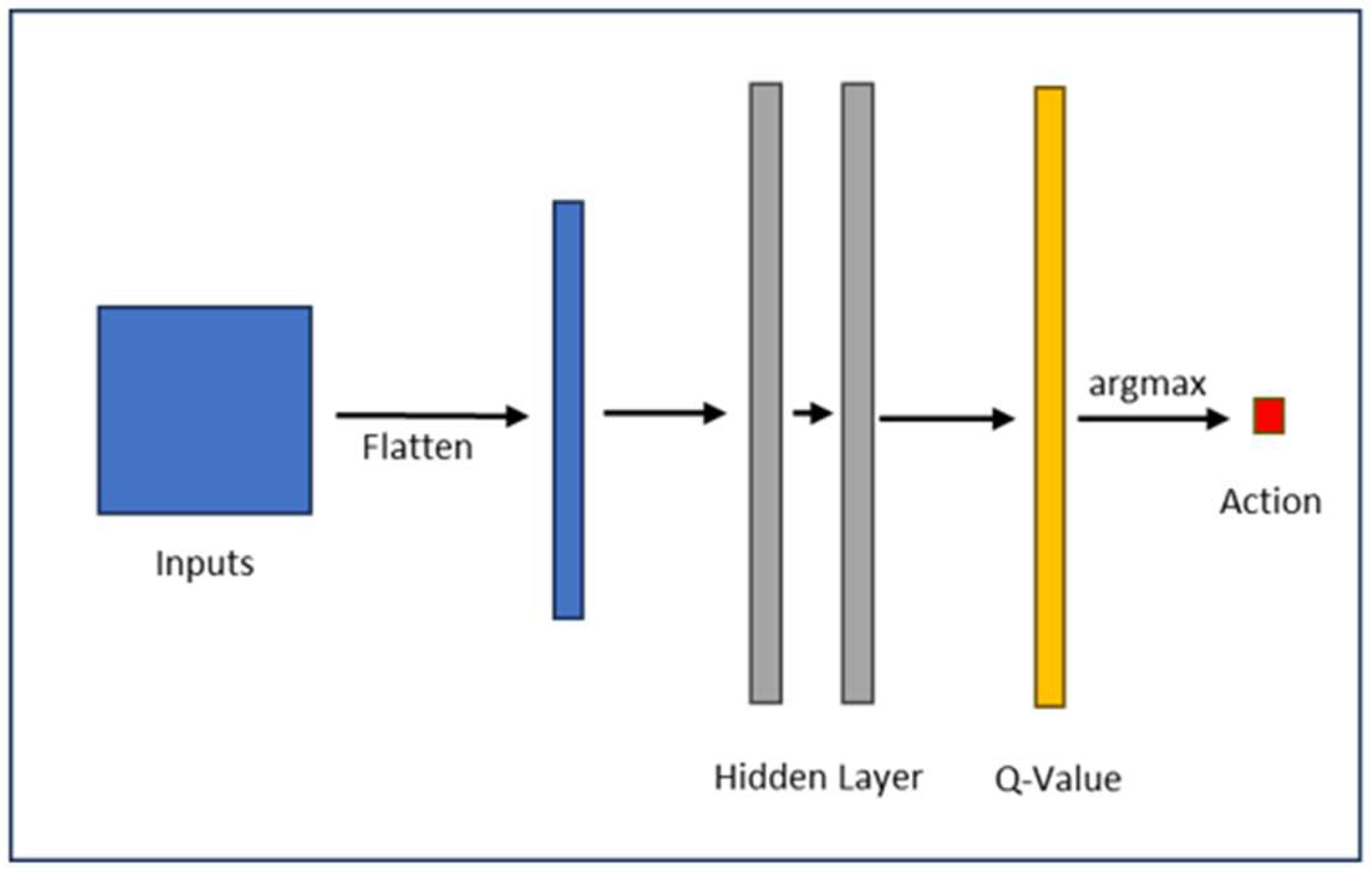
2.3. Deep-Reinforcement-Learning

Markov Decision Process (MDP) is a framework used in modeling sequential decision-making problems. In an MDP, the system evolves over time by selecting actions based on the current state. The goal is to find an optimal policy that can maximize long-term cumulative reward. Autonomous driving naturally fits into this framework. At each moment, driving decisions such as whether to change lanes, accelerate, or slow down are made based on the current vehicle state and traffic environment. Therefore, in this paper, we formulate the high-level autonomous driving task as an MDP, and the detailed MDP setting is provided in the case study section.

Once the autonomous diving problem is formulated using MDP, reinforcement learning (RL) can then be employed to optimize the decision-making process and find an optimal policy. Deep Reinforcement Learning (DRL), a subset of RL, is particularly effective for autonomous driving applications and can be broadly categorized into value-based and policy-based methods. Value-based DRL, inspired by Q-learning [43], estimates action values to determine the best possible decision. Techniques such as Deep Q-Networks (DQN), Double Deep Q-Networks (DDQN), and their successor [44,45,46,47] improve learning efficiency in environments with large state spaces and discrete action spaces. Policy-based DRL [48], on the other hand, directly learns a mapping from states to actions without explicitly estimating value functions. Methods such as Policy Gradient (PG), Actor-Critic (A2C [49], A3C [50]), Proximal Policy Optimization (PPO) [51], and their successor [52,53,54] refine decision-making by adjusting policy parameters to maximize expected rewards.

In this paper, since the high-level decision-making agent is required to generate discrete lane-level actions, a value-based reinforcement learning method is particularly well-suited. Compared with policy-based methods, value-based approaches like Q-learning and its variants tend to be more sample-efficient and easier to train in discrete action spaces. Given the relatively simple structure of our task and the need for stable and efficient learning, we adopt the DDQN algorithm to train the high-level agent. From the loss function of DDQN shown in Equation (26), DDQN mitigates the overestimation bias found in standard DQN by decoupling action selection and action evaluation during Q-value updates (using $\underset{a_{t+1}}{\mathit{max}}{Q}_{{\theta }_i^{-}}\left(s_{t+1},\mathit{arg}\underset{a_{t+1} }{\mathit{max}}{Q}_{{\theta }_i}(s_{t+1},a_{t+1})\right)$ instead of $\underset{a_{t+1} }{\mathit{max}}{Q}_{{\theta }_i^{-}}(s_{t+1},a_{t+1})$ for update), leading to a more stable training process.

Table 2. DDQN loss function parameters.

Symbol	Parameter
$s$	State
$a$	Action
$r$	Immediate reward
${\theta }_i^{-}$	Target-network’s parameter
${\theta }_i$	Online-network’s parameter
$\gamma$	Discount for future reward

provides detailed explanation of the parameters in loss functions. Moreover, while DDQN is used in this work due to its simplicity and effectiveness, the modular design of our hierarchical framework allows for flexibility. For complex driving tasks, more advanced algorithms such as SAC or DDPG can be applied for better performance.

$$L_i\left(\theta \right)={\mathbb{E}}_{(s,a,r)}\left[{\left(r+\gamma \underset{a_{t+1}}{\mathit{max}}{Q}_{{\theta }_i^{-}}\left(s_{t+1},\mathit{arg}\underset{a_{t+1} }{\mathit{max}}{Q}_{{\theta }_i}(s_{t+1},a_{t+1})\right)-Q_{{\theta }_i}(s_t,a_t)\right)}^2\right]$$

(26)

Figure 2 illustrates the neural network structure used in the DDQN framework and Algorithm 1 demonstrates the pseudocode of hierarchical DDQN implementation in this paper. The DDQN employs a fully connected feedforward neural network consisting of two hidden layers, each with 128 neurons using ReLU as activation functions. The input layer has 25 units (flattened from 5 × 5 including ego vehicle’s information and traffic environment information), and the output layer has 3 units corresponding to three lane-level actions. The training process uses a standard replay buffer with a size of 100,000 and a mini-batch size of 64. The Q-network is updated using the mean squared error (MSE) loss between the predicted Q-values and the target Q-values. The Adam optimizer is used with a learning rate of 0.001. To stabilize training and mitigate overestimation bias, a target network is maintained and synchronized with the main Q-network every 100 learning steps. An $\epsilon$-greedy exploration strategy is adopted, where $\epsilon$ linearly decays from 1.0 to 0.05 over 200,000 steps. This linear decay strategy allows the agent to fully explore the environment instead of converging to a local optimal policy.

Algorithm 1: Hierarchical DDQN algorithm flowchart

1: Initialize high-level DDQN agent

2: Initialize low-level HOCLF-HOCBF-QP controller

3: for each episode do

4:       Initialize and reset traffic environment

5:       for t = 1 to T do

6:             With probability $ϵ$ select a random high-level action $a_t$

7:             Otherwise select high-level action $a_t={\mathrm{m}\mathrm{a}\mathrm{x}}_{\mathrm{a}}{Q}^{\ast }(s_t,a;\theta )$

8:             for each low-level control steps do

9:                   Reset target tracking point according to current states and $a_t$

10:                   Reset obstacle list according to current states

11:                   Calculate optimal control $u^{\ast }$ using HOCLF-HOCBF-QP

12:                   Execute $u^{\ast }$ for a control step

13:             end for

14:             Calculate reward $r_t$ and record next state $s_{t+1}$

15:             Store transition ($s_t$, $a_t$, $r_t$, $s_{t+1}$) in replay buffer $D$

16:             if t mod training frequency == 0 then

17:                   Sample random minibatch of transitions ($s_j$, $a_j$, $r_j$, $s_{j+1}$)) from D

18:                   Set $y_j=r_j+\gamma {{max}_a}_{j+1}\widehat{Q}(s_{j+1},{{argmax}_a}_{j+1}Q(s_j,a_{j+1};\theta );\theta )$

19:                   for non-terminal $s_{j+1}$

20:                   or $y_j=r_j$ for terminal $s_{j+1}$

21:                   Perform a gradient descent step to update $\theta$

22:                   Every N steps reset $\widehat{Q}$ = $Q$

23:             end if

24:             Set $s_{t+1}$ = $s_t$

25:        end for

26: end for

3. Results

In this section, we present simulation results of the proposed hierarchical control framework to evaluate its effectiveness and robustness. The results are organized into two parts to demonstrate both the individual performance of the low-level HOCLF-HOCBF-QP-based controller and the overall system performance after combining with the high-level DDQN-based decision-making agent.

Table 3. Value of parameters used in simulation.

Symbol	Parameter	Value
$V$	Center-of-gravity (CG) velocity	5 m/s
m	Mass	3000 kg
$I_z$	Yaw moment of inertia	5.113 × 103 kg m2
$C_f$	Front tire cornering stiffness	3 × 105 N/rad
$C_r$	Rear tire cornering stiffness	3 × 105 N/rad
$l_f$	Distance between CG and front axle	2 m
$l_r$	Distance between CG and rear axle	2 m
${\delta }_{fmax}$	Maximum allowed front wheel steer angle	0.7 rad
${\delta }_{fmin}$	Minimum allowed front wheel steer angle	−0.7 rad

displays the values of the parameters used in the simulations.

3.1. CLF-CBF-Based Optimization Controller

To prove the effectiveness of the proposed low-level controller, we conduct simulations to evaluate the performance of the HOCLF-HOCBF-QP controller in both path tracking and collision avoidance. We first test the HOCLF-QP controller’s tracking performance using a reference path tracking test case. In this test case, the vehicle is required to travel from a starting point to a destination while following a predefined reference trajectory. The results show that the proposed HOCLF design allows the vehicle to smoothly and accurately follow the predefined path in obstacle-free environments.

Then, we incorporate HOCBF constraints into the controller and evaluate the controller’s collision avoidance capability. An obstacle is deliberately placed near the reference path to test whether the controller can successfully avoid potential collisions by temporarily deviating from the planned trajectory. Simulation results indicate successful navigation around the obstacle and smooth return to the reference path once the obstacle is safely passed. In addition, we also evaluate the controller’s capability to perform reference point tracking. In this test case, the vehicle starts from an arbitrary starting point and is required to reach a target reference point while avoiding surrounding obstacles. The simulation results demonstrate that the proposed HOCLF-HOCBF-QP controller can effectively perform path planning and ensure real-time safety in complex dynamic environments with multiple obstacles.

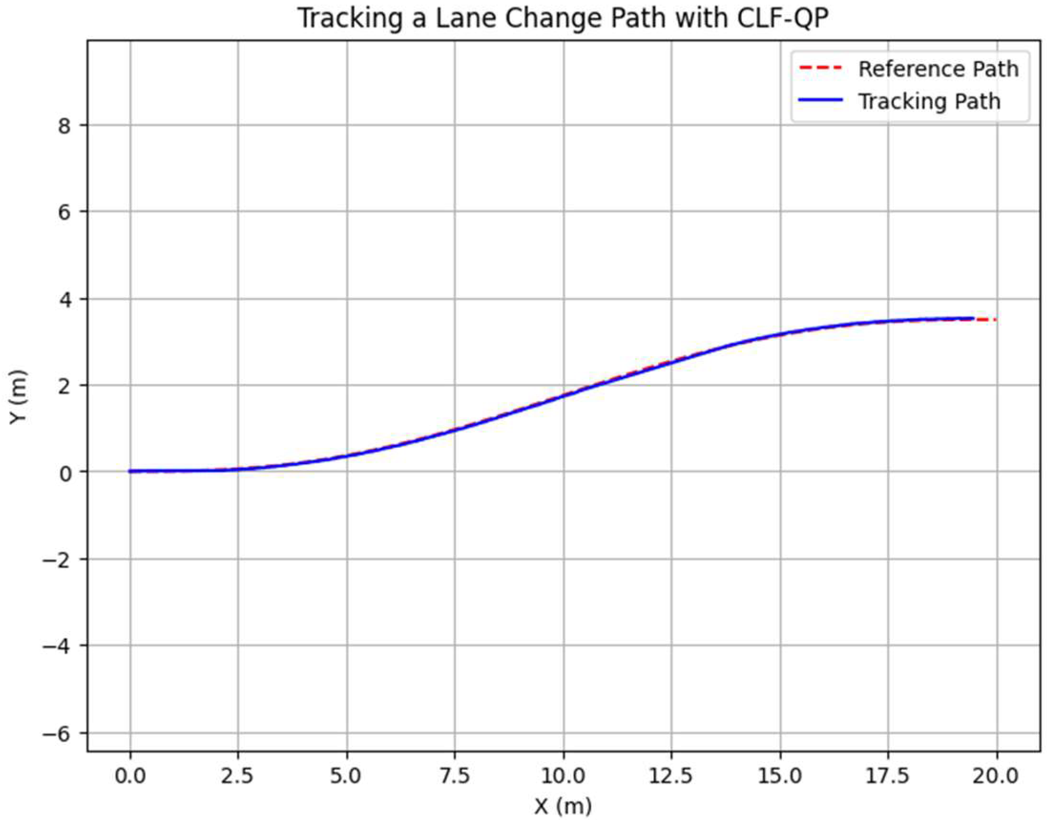
3.1.1. CLF-Based Path Tracking Controller

Figure 3 shows the tracking performance of the HOCLF-QP controller on a predefined single lane change reference trajectory. The red dashed line represents the desired reference path of the single lane change maneuver, while the blue solid line illustrates the actual trajectory of the ego vehicle under the HOCLF-QP control. As observed in the figure, the tracking performance is highly accurate throughout the entire path. The controller successfully leads the vehicle to follow the reference path with minimal lateral deviation, indicating the effectiveness of the HOCLF formulation in ensuring the stability of the system. This result validates the controller’s ability to serve as a reliable low-level trajectory tracking controller for use in the proposed hierarchical control framework.

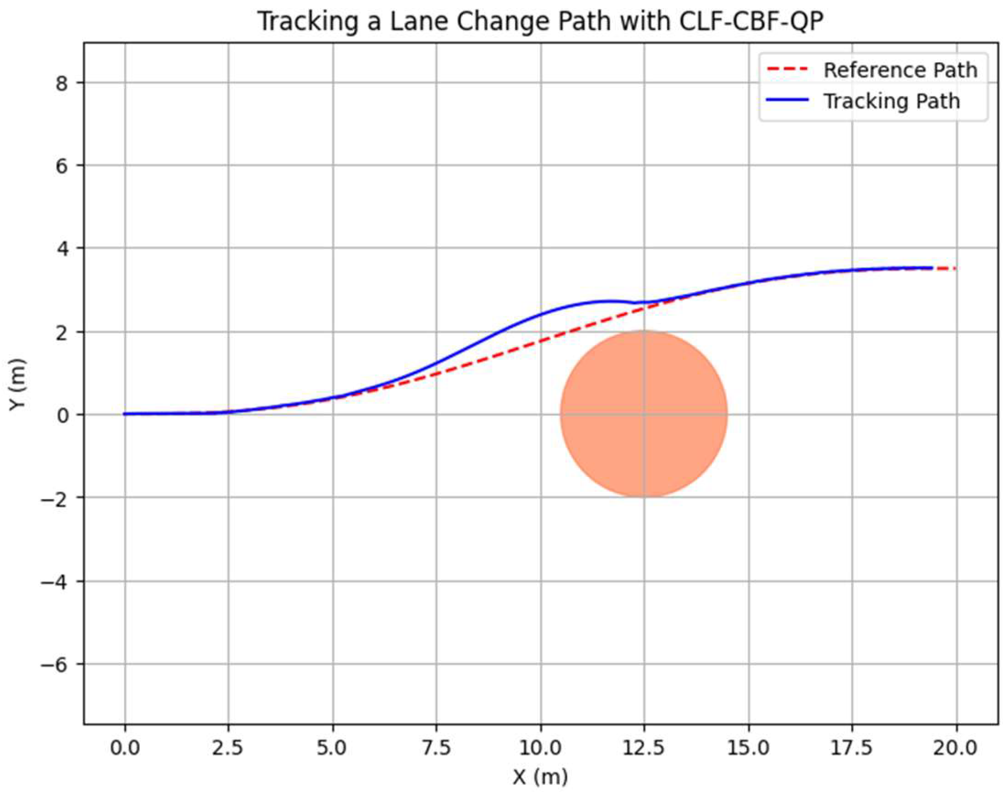
3.1.2. CLF-CBF-Based Autonomous Driving Controller for Static Obstacle

Figure 4 shows the trajectory tracking result of the HOCLF-HOCBF-QP controller in the presence of a static obstacle. The red dashed line represents the original reference path of the single lane change maneuver, while the orange circle represents the obstacle that is deliberately added near the predefined path. The blue line represents the actual trajectory of the ego vehicle under the HOCLF-HOCBF-QP control. Compared to the HOCLF-QP controller results, which focused only on trajectory tracking, as demonstrated in the previous section, the HOCLF-HOCBF-QP controller successfully leads the vehicle to change its trajectory to avoid potential collision with the obstacle while still tracking the desired path after passing the obstacle. The safety constraint is enforced by HOCBF, which ensures that the system state remains within a safe set even when the original reference would result in a potential collision. The deviation from the reference path is observed near the obstacle, which is an intentional and necessary result of the CBF-based safety intervention. Once the vehicle passes the obstacle, it smoothly returns to its reference trajectory, demonstrating the controller’s ability to balance safety and stability.

Figure 5 illustrates the reference point tracking performance of the HOCLF-HOCBF-QP controller in a complex environment with multiple static obstacles. The vehicle starts from origin and aims to reach a predefined destination (represented by the green marker) while avoiding collisions with the circular obstacles (represented by the orange circles). The dashed line shows the actual trajectory of the ego vehicle under the HOCLF-HOCBF-QP control, which demonstrates the controller’s ability to balance target point tracking and obstacle avoidance. Notably, the trajectory deviates smoothly around all three obstacles, indicating that the HOCBF constraints are effectively preventing the system from entering unsafe sets. This test case proves the effectiveness of the HOCLF-HOCBF-QP controller in reference point tracking and collision avoidance tasks, particularly in complex environments with multiple obstacles. This result further validates the controller’s ability to serve as a reliable low-level trajectory tracking module in the proposed hierarchical control framework.

3.1.3. CLF-CBF-Based Autonomous Driving Controller for Dynamic Obstacle

To further evaluate the low-level HOCLF-HOCBF-QP controller’s collision avoidance capability, we tested its performance in a traffic scenario involving a dynamic obstacle moving along a predefined single-lane-changing trajectory. Figure 6 shows the trajectory tracking result of the HOCLF-HOCBF-QP controller in the presence of a dynamic obstacle. The ego vehicle successfully tracked the reference path before and after the interaction with obstacles while performing a clear collision avoidance maneuver when approaching the obstacle. During the avoidance process, the vehicle deviated from the reference path to maintain safety but smoothly rejoined the original trajectory once the obstacle was passed.

Figure 7 illustrates the real-time distance between the vehicle and the dynamic obstacle over time. The minimum distance occurs at around 2.0 s, where the vehicle and the obstacle are at their closest. The minimum distance remains above the predefined safety threshold of 2 m, which is generally considered a socially acceptable minimum safe distance between vehicles and surrounding objects in typical driving scenarios.

3.2. Hybrid DRL and CLF-CBF-Based Controller

In this section, we present the simulation results of the proposed hierarchical control framework, which integrates a high-level DDQN-based decision-making agent and a low-level HOCLF-HOCBF-QP-based trajectory tracking controller. After validating the effectiveness of the low-level controller in the previous section, we integrate a high-level planner to handle more complex decision-making tasks. To evaluate the overall performance of the hierarchical control framework, we design a simple and complex test case within a multi-lane traffic environment. In both cases, the ego vehicle must travel from a starting point to a predefined destination, navigating through a roadway populated with multiple obstacles. The vehicle is required to dynamically avoid obstacles by performing appropriate lane changes. The test cases are constructed using a highway-environment simulator [55]. The environment settings, vehicle dynamics, and the low-level control strategy are modified to match our problem setup. Unlike traditional trajectory planning setups, no predefined global path is provided. Instead, the DDQN-based high-level agent generates discrete lane-level decisions (e.g., idle, left lane change, right lane change) based on observation of the ego vehicle’s state and the traffic environment. At the same time, the HOCLF-HOCBF-QP low-level controller ensures that each decision is executed safely and accurately in real time.

In this paper, the environment state is represented as a 5 × 5 array that encodes information about the ego vehicle and its surrounding obstacles. Each row corresponds to an entity (either the ego vehicle or an obstacle) and includes the following attributes: [presence, $x$, $y$, $v_x$, $v_y$], where presence is a binary indicator of whether the object exists in the current frame. The action space is discrete and consists of three possible maneuvers: idle (no lane change), left lane change, and right lane change. The reward function is designed to encourage goal-reaching behavior while penalizing unsafe or inefficient actions. A positive reward of +50 is assigned when the vehicle successfully reaches its destination. A large negative reward of −100 is applied in the event of a collision with any obstacle. Additionally, at each timestep, the agent receives a dense reward proportional to its forward progress ($∆x$), calculated as $r_{progress}=c\ast (x_{current}-x_{prev})$, where $c$ is a positive coefficient, which encourages faster navigation. A small penalty of −0.5 is applied when the agent executes a lane change (either left or right) to discourage unnecessary lateral movement and to promote trajectory stability.

Simulation results from both test cases show that the proposed framework can make the vehicle successfully navigate from the start point to its destination while effectively avoiding all obstacles using the appropriate lane-changing maneuver(s).

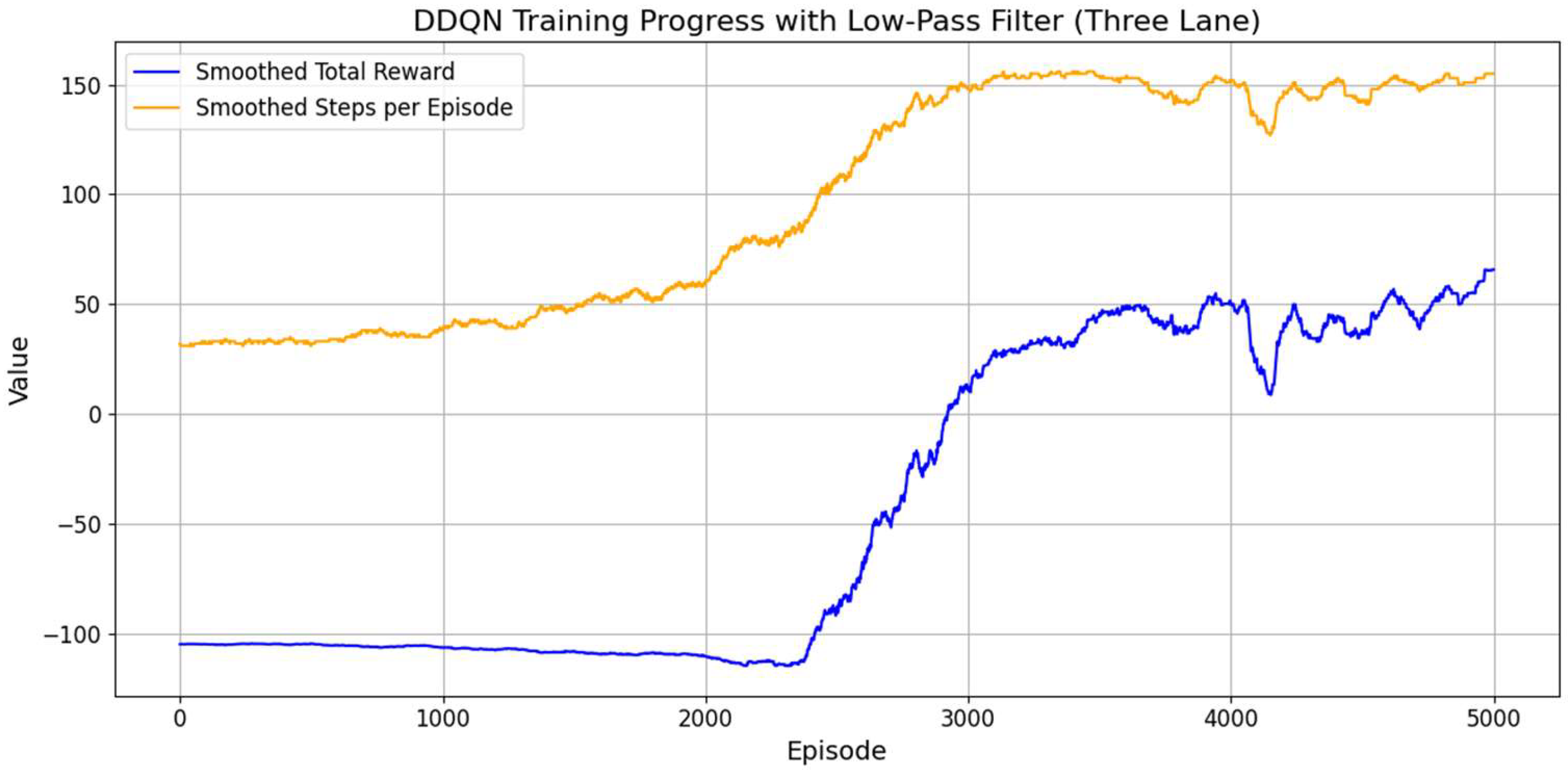
3.2.1. DRL High-Level Decision-Making Agent

In this section, we first present the training progress of the high-level DDQN-based decision-making agent in the proposed hierarchical control framework.

Table 4. Hyperparameters and training settings.

Hyperparameter	Value
Replay buffer size	100,000
Mini-batch size	64
Learning rate	0.001
Target network update frequency	Every 100 steps
Exploration strategy (ε decay)	1.0 → 0.05 over 200,000 steps
Discount factor (γ)	0.99
Optimizer	Adam
Loss function	Mean Squared Error (MSE)

summarizes the key hyperparameters used in the DDQN training process, and Figure 8 illustrates the training progress of the DDQN high-level decision-making agent in the three-lane complex autonomous driving environment. A low-pass filter is applied to smooth both the episode reward and step count curves for better interpretability. Initially, the agent exhibits poor performance due to the high probability of random explorations, with the total reward remaining negative and the step count relatively low, indicating frequent collisions and early episode terminations. After approximately 2500 episodes, a significant improvement is observed: The total reward begins to rise rapidly, and the average number of steps per episode increases concurrently. This trend suggests that the agent gradually learns an effective lane-changing strategy to avoid obstacles and to extend its episode longevity. After about 3500 episodes, both rewards and steps per episode are maintained at a relatively high level, indicating convergence to a stable policy. Some fluctuations are still present in the reward curve, likely due to exploration behavior or occasional difficult scenarios.

3.2.2. Hybrid DRL and CLF-CBF Controller

Figure 9 illustrates the ego vehicle’s trajectory in a two-lane highway test case using the proposed hierarchical controller. The road is divided into two lanes with clearly marked boundaries and a centerline. The ego vehicle (represented by the yellow rectangle) starts in the upper lane and initially follows a straight path before encountering an obstacle (represented by the red rectangle) positioned ahead in the same lane. The vehicle performs a lane-change maneuver in front of the obstacle by smoothly transitioning into the lower lane. After passing the obstacle, the vehicle performs another lane-change maneuver and returns to the upper lane to avoid collision with the second obstacle. A video animation of the two-lane test case is available at https://youtu.be/a1442r2Rg-E (accessed on 9 June 2025).

Figure 10 illustrates the ego vehicle’s trajectory in a complex three-lane highway test case using the proposed hierarchical controller. From the plot, we notice that this environment is much more complex compared to the simple two-lane test case demonstrated before. The ego vehicle (represented by the yellow rectangle) starts in the upper lane and initially follows a straight path before encountering an obstacle (represented by the red rectangle) positioned ahead in the same lane. The vehicle performs two consecutive lane-change maneuvers to transition smoothly into the lower lane in response to a series of obstacles. After passing the obstacles, the vehicle performs another two consecutive lane-change maneuvers and returns to the upper lane to avoid collision with other obstacles. A video animation of the two-lane test case is available at https://youtu.be/t3RXrZ1A7XU (accessed on 9 June 2025).

The two trajectory plots in Figure 9 and Figure 10 demonstrate the effectiveness of the proposed hierarchical control system. The high-level DDQN agent can correctly generate lane-change decisions based on obstacle positions, while the low-level HOCLF-HOCBF-QP controller ensures smooth and safe high-level decision execution. The trajectory remains continuous and collision-free throughout the simulation, indicating successful integration of decision-making and control components. Moreover, the vehicle consistently follows a straight path in obstacle-free regions, without performing unnecessary lane-change behaviors. This suggests that the penalty design for lane changes successfully discourages unnecessary lane-changing actions, which makes the decision-making process more efficient.

To evaluate the computational efficiency of the proposed hierarchical control framework, we conducted computational cost tests based on the aforementioned simulation test case. In complex test case settings, the low-level control simulation frequency is 100 Hz and the high-level policy simulation frequency is 5 Hz. The low-level HOCLF-HOCBF-QP controller requires an average solve time of approximately 0.66 ms per step using the Gurobi optimizer, while the high-level DDQN decision-making agent requires an average computational time of approximately 0.60 ms per step. These tests were performed in a Google Colab CPU environment, which is using a single-threaded Intel Xeon, and there is no GPU acceleration. Even under this relatively limited computational setting, the solve times account for only 6.6% of the low-level control cycle (10 ms) and 0.3% of the high-level decision-making cycle (200 ms), respectively. These results demonstrate that the proposed framework has good real-time capability. While it is expected that the computational time, particularly for the HOCLF-HOCBF-QP controller, will increase in more complex traffic scenarios with higher numbers of obstacles and constraints, our current results suggest that the proposed framework still provides sufficient real-time capability for typical autonomous driving tasks. In future work, we plan to further evaluate its effectiveness and real-time capability by conducting tests using the Hardware-in-the-Loop (HIL) approach and Vehicle-in-Virtual-Environment (VVE) approach to ensure its real-world feasibility and practical applicability in different driving scenarios.

4. Conclusions and Future Work

Path planning and collision avoidance are critical challenges in the development of reliable autonomous driving systems, particularly in dynamic multi-lane environments with obstacles. Traditional rule-based planners often struggle to handle such complexities. To address these limitations, this paper proposed a hierarchical decision-making and control framework that enables autonomous vehicles to automatically avoid obstacles through lane-changing maneuvers.

The proposed system integrates a high-level DDQN-based decision-making agent with a low-level HOCLF-HOCBF-QP-based controller. The high-level DDQN agent generates discrete lane-level decisions based on the ego vehicle’s information and traffic environment information, while the HOCLF-HOCBF-QP controller ensures safe and efficient trajectory tracking and collision avoidance.

Simulation results validate the effectiveness of the framework in navigating complex multi-lane traffic environments with static obstacles. The results show that the system can successfully execute appropriate lane-changing maneuvers to avoid collisions while navigating from starting point to destination.

In addition to demonstrating collision avoidance performance, we also evaluated the computational efficiency of the proposed framework. Computational cost tests show that the low-level HOCLF-HOCBF-QP controller and the high-level DDQN agent complete their respective computations well within the control cycles. These results demonstrate that the framework has real-time performance capability for autonomous driving applications.

Compared to traditional optimization-based methods such as model predictive control (MPC), the proposed framework significantly simplifies the online optimization process. Traditional approaches typically solve large-scale optimal control problems at each step, which introduces high computational complexity and often requires accurate environmental modeling. Also, these approaches sometimes may struggle to find optimal paths in complex traffic conditions. In contrast, our approach takes advantage of the high-level DRL-based decision-making agent and further enhances the system’s capability to navigate various complex traffic environments. In addition, compared to traditional reinforcement learning methods [56,57], including end-to-end approaches, the key advantage of our proposed framework lies in the explicit integration of a low-level controller, which ensures hard-coded safety rules. Traditional RL methods rely entirely on reward design and learned policies to avoid collisions, which can still lead to unsafe behaviors during training or in unforeseen situations, as they lack hard safety guarantees. In contrast, our approach separates decision-making and low-level control. The high-level DDQN agent focuses on discrete lane-level maneuver selection, leveraging the adaptability and learning capability of RL to handle diverse traffic conditions. Meanwhile, the low-level HOCLF-HOCBF-QP controller ensures safety by introducing CBF constraint, providing a hard-coded safety layer.

There are still some limitations in this study. First, the vehicle model used in this work is based on linear lateral dynamics with constant longitudinal speed, which limits the realism of driving behavior. Future work will consider integrating a longitudinal dynamic model to capture the vehicle’s longitudinal motions, hence letting the model become a full vehicle dynamic model. Second, although DDQN performs well in the current setup, more advanced DRL algorithms such as SAC or DDPG could potentially improve learning efficiency and policy robustness in more complex or uncertain environments, and their use will also be investigated in future work. Finally, we plan to conduct more detailed sensitivity analyses and ablation studies to further understand the impact of key parameters and the contribution of each module, especially in more complex dynamic environments with multiple road users.

References

1. Wen, B.; Gelbal, S.; Aksun-Guvenc, B.; Guvenc, L. Localization and Perception for Control and Decision Making of a Low Speed Autonomous Shuttle in a Campus Pilot Deployment. arXiv 2018, arXiv:2407.00820. [Google Scholar] [CrossRef]
2. Gelbal, S.Y.; Guvenc, B.A.; Guvenc, L. SmartShuttle: A unified, scalable and replicable approach to connected and automated driving in a smart city. In Proceedings of the 2nd International Workshop on Science of Smart City Operations and Platforms Engineering, in SCOPE ’17, Pittsburgh, PA, USA, 18–21 April 2017; Association for Computing Machinery: New York, NY, USA, 2017; pp. 57–62. [Google Scholar] [CrossRef]
3. “Autonomous Road Vehicle Path Planning and Tracking Control | IEEE eBooks | IEEE Xplore”. Available online: https://ieeexplore.ieee.org/book/9645932 (accessed on 24 October 2023).
4. Ararat, O.; Aksun-Guvenc, B. Development of a Collision Avoidance Algorithm Using Elastic Band Theory. IFAC Proc. Vol. 2008, 41, 8520–8525. [Google Scholar] [CrossRef]
5. Ames, A.D.; Grizzle, J.W.; Tabuada, P. Control barrier function based quadratic programs with application to adaptive cruise control. In Proceedings of the 53rd IEEE Conference on Decision and Control, Los Angeles, CA, USA, 15–17 December 2014; pp. 6271–6278. [Google Scholar] [CrossRef]
6. Ames, A.D.; Xu, X.; Grizzle, J.W.; Tabuada, P. Control Barrier Function Based Quadratic Programs for Safety Critical Systems. IEEE Trans. Autom. Control. 2017, 62, 3861–3876. [Google Scholar] [CrossRef]
7. Ames, A.D.; Coogan, S.; Egerstedt, M.; Notomista, G.; Sreenath, K.; Tabuada, P. Control Barrier Functions: Theory and Applications. In Proceedings of the 2019 18th European Control Conference (ECC), Naples, Italy, 25–28 June 2019; pp. 3420–3431. [Google Scholar] [CrossRef]
8. Wang, L.; Ames, A.D.; Egerstedt, M. Safety Barrier Certificates for Collisions-Free Multirobot Systems. IEEE Trans. Robot. 2017, 33, 661–674. [Google Scholar] [CrossRef]
9. Desai, M.; Ghaffari, A. CLF-CBF Based Quadratic Programs for Safe Motion Control of Nonholonomic Mobile Robots in Presence of Moving Obstacles. In Proceedings of the 2022 IEEE/ASME International Conference on Advanced Intelligent Mechatronics (AIM), Sapporo, Japan, 11–15 July 2022; pp. 16–21. [Google Scholar] [CrossRef]
10. Reis, M.F.; Andrade, G.A.; Aguiar, A.P. Safe Autonomous Multi-vehicle Navigation Using Path Following Control and Spline-Based Barrier Functions. In Robot 2023: Sixth Iberian Robotics Conference; Marques, L., Santos, C., Lima, J.L., Tardioli, D., Ferre, M., Eds.; Springer: Cham, Switzerland, 2024; pp. 297–309. [Google Scholar] [CrossRef]
11. Yang, G.; Vang, B.; Serlin, Z.; Belta, C.; Tron, R. Sampling-based Motion Planning via Control Barrier Functions. In Proceedings of the 2019 3rd International Conference on Automation, Control and Robots, Prague, Czech Republic, 11–13 October 2019; pp. 22–29. [Google Scholar] [CrossRef]
12. Li, Y.; Peng, Z.; Liu, L.; Wang, H.; Gu, N.; Wang, A.; Wang, D. Safety-Critical Path Planning of Autonomous Surface Vehicles Based on Rapidly-Exploring Random Tree Algorithm and High Order Control Barrier Functions. In Proceedings of the 2023 8th International Conference on Automation, Control and Robotics Engineering (CACRE), Guangzhou, China, 13–15 July 2023; pp. 203–208. [Google Scholar] [CrossRef]
13. He, S.; Zeng, J.; Zhang, B.; Sreenath, K. Rule-Based Safety-Critical Control Design using Control Barrier Functions with Application to Autonomous Lane Change. arXiv 2021, arXiv:2103.12382. [Google Scholar] [CrossRef]
14. Liu, M.; Kolmanovsky, I.; Tseng, H.E.; Huang, S.; Filev, D.; Girard, A. Potential Game-Based Decision-Making for Autonomous Driving. arXiv 2023, arXiv:2201.06157. [Google Scholar] [CrossRef]
15. Jabbari, F.; Samsami, R.; Arefi, M.M. A Novel Online Safe Reinforcement Learning with Control Barrier Function Technique for Autonomous vehicles. In Proceedings of the 2024 10th International Conference on Control, Instrumentation and Automation (ICCIA), Kashan, Iran, 5–7 November 2024; pp. 1–6. [Google Scholar] [CrossRef]
16. Chen, X.; Liu, X.; Zhang, M. Autonomous Vehicle Lane-Change Control Based on Model Predictive Control with Control Barrier Function. In Proceedings of the 2024 IEEE 13th Data Driven Control and Learning Systems Conference (DDCLS), Kaifeng, China, 17–19 May 2024; pp. 1267–1272. [Google Scholar] [CrossRef]
17. Thirugnanam, A.; Zeng, J.; Sreenath, K. Safety-Critical Control and Planning for Obstacle Avoidance between Polytopes with Control Barrier Functions. arXiv 2022, arXiv:2109.12313. [Google Scholar] [CrossRef]
18. Xiao, W.; Belta, C. High-Order Control Barrier Functions. IEEE Trans. Autom. Control. 2022, 67, 3655–3662. [Google Scholar] [CrossRef]
19. Chriat, A.E.; Sun, C. High-Order Control Lyapunov–Barrier Functions for Real-Time Optimal Control of Constrained Non-Affine Systems. Mathematics 2024, 12, 24. [Google Scholar] [CrossRef]
20. Wang, H.; Tota, A.; Aksun-Guvenc, B.; Guvenc, L. Real time implementation of socially acceptable collision avoidance of a low speed autonomous shuttle using the elastic band method. Mechatronics 2018, 50, 341–355. [Google Scholar] [CrossRef]
21. Lu, S.; Xu, R.; Li, Z.; Wang, B.; Zhao, Z. Lunar Rover Collaborated Path Planning with Artificial Potential Field-Based Heuristic on Deep Reinforcement Learning. Aerospace 2024, 11, 253. [Google Scholar] [CrossRef]
22. Morsali, M.; Frisk, E.; Åslund, J. Spatio-Temporal Planning in Multi-Vehicle Scenarios for Autonomous Vehicle Using Support Vector Machines. IEEE Trans. Intell. Veh. 2021, 6, 611–621. [Google Scholar] [CrossRef]
23. Zhu, S. Path Planning and Robust Control of Autonomous Vehicles. Ph.D. Thesis, The Ohio State University, Columbus, OH, USA, 2020. Available online: https://www.proquest.com/docview/2612075055/abstract/73982D6BAE3D419APQ/1 (accessed on 24 October 2023).
24. Chen, G.; Yao, J.; Gao, Z.; Gao, Z.; Zhao, X.; Xu, N.; Hua, M. Emergency Obstacle Avoidance Trajectory Planning Method of Intelligent Vehicles Based on Improved Hybrid A*. SAE Int. J. Veh. Dyn. Stab. NVH 2023, 8, 3–19. [Google Scholar] [CrossRef]
25. Kiran, B.R.; Sobh, I.; Talpaert, V.; Mannion, P.; Al Sallab, A.A.; Yogamani, S.; Perez, P. Deep Reinforcement Learning for Autonomous Driving: A Survey. IEEE Trans. Intell. Transp. Syst. 2022, 23, 4909–4926. [Google Scholar] [CrossRef]
26. Ye, F.; Zhang, S.; Wang, P.; Chan, C.-Y. A Survey of Deep Reinforcement Learning Algorithms for Motion Planning and Control of Autonomous Vehicles. In Proceedings of the 2021 IEEE Intelligent Vehicles Symposium (IV), Nagoya, Japan, 11–17 July 2021; pp. 1073–1080. [Google Scholar] [CrossRef]
27. Zhu, Z.; Zhao, H. A Survey of Deep RL and IL for Autonomous Driving Policy Learning. IEEE Trans. Intell. Transp. Syst. 2022, 23, 14043–14065. [Google Scholar] [CrossRef]
28. Kendall, A.; Hawke, J.; Janz, D.; Mazur, P.; Reda, D.; Allen, J.-M.; Lam, V.-D.; Bewley, A.; Shah, A. Learning to Drive in a Day. arXiv 2018, arXiv:1807.00412. [Google Scholar] [CrossRef]
29. Yurtsever, E.; Capito, L.; Redmill, K.; Ozguner, U. Integrating Deep Reinforcement Learning with Model-based Path Planners for Automated Driving. arXiv 2020, arXiv:2002.00434. [Google Scholar] [CrossRef]
30. Aksjonov, A.; Kyrki, V. A Safety-Critical Decision-Making and Control Framework Combining Machine-Learning-Based and Rule-Based Algorithms. SAE Int. J. Veh. Dyn. Stab. NVH 2023, 7, 287–299. [Google Scholar] [CrossRef]
31. “Deep Reinforcement-Learning-Based Driving Policy for Autonomous Road Vehicles—Makantasis—2020—IET Intelligent Transport Systems—Wiley Online Library”. Available online: https://ietresearch.onlinelibrary.wiley.com/doi/full/10.1049/iet-its.2019.0249 (accessed on 24 October 2023).
32. Merola, F.; Falchi, F.; Gennaro, C.; Di Benedetto, M. Reinforced Damage Minimization in Critical Events for Self-driving Vehicles. In Proceedings of the 17th International Joint Conference on Computer Vision, Imaging and Computer Graphics Theory and Applications, Lisbon, Portugal, 19–21 February 2023; pp. 258–266. [Google Scholar] [CrossRef]
33. Nageshrao, S.; Tseng, H.E.; Filev, D. Autonomous Highway Driving using Deep Reinforcement Learning. In Proceedings of the 2019 IEEE International Conference on Systems, Man and Cybernetics (SMC), Bari, Italy, 6–9 October 2019; pp. 2326–2331. [Google Scholar] [CrossRef]
34. Peng, B.; Sun, Q.; Li, S.E.; Kum, D.; Yin, Y.; Wei, J.; Gu, T. End-to-End Autonomous Driving Through Dueling Double Deep Q-Network. Automot. Innov. 2021, 4, 328–337. [Google Scholar] [CrossRef]
35. Cao, Z.; Biyik, E.; Wang, W.; Raventos, A.; Gaidon, A.; Rosman, G.; Sadigh, D. Reinforcement Learning based Control of Imitative Policies for Near-Accident Driving. arXiv 2020, arXiv:2007.00178. [Google Scholar] [CrossRef]
36. Jaritz, M.; de Charette, R.; Toromanoff, M.; Perot, E.; Nashashibi, F. End-to-End Race Driving with Deep Reinforcement Learning. arXiv 2018, arXiv:1807.02371. [Google Scholar] [CrossRef]
37. Ashwin, S.H.; Raj, R.N. Deep reinforcement learning for autonomous vehicles: Lane keep and overtaking scenarios with collision avoidance. Int. J. Inf. Tecnol. 2023, 15, 3541–3553. [Google Scholar] [CrossRef]
38. Muzahid, A.J.M.; Kamarulzaman, S.F.; Rahman, M.A.; Alenezi, A.H. Deep Reinforcement Learning-Based Driving Strategy for Avoidance of Chain Collisions and Its Safety Efficiency Analysis in Autonomous Vehicles. IEEE Access 2022, 10, 43303–43319. [Google Scholar] [CrossRef]
39. Dinh, L.; Quang, P.T.A.; Leguay, J. Towards Safe Load Balancing based on Control Barrier Functions and Deep Reinforcement Learning. arXiv 2024, arXiv:2401.05525. [Google Scholar] [CrossRef]
40. Chen, H.; Zhang, F.; Aksun-Guvenc, B. Collision Avoidance in Autonomous Vehicles Using the Control Lyapunov Function–Control Barrier Function–Quadratic Programming Approach with Deep Reinforcement Learning Decision-Making. Electronics 2025, 14, 557. [Google Scholar] [CrossRef]
41. Chen, H.; Cao, X.; Guvenc, L.; Aksun-Guvenc, B. Deep-Reinforcement-Learning-Based Collision Avoidance of Autonomous Driving System for Vulnerable Road User Safety. Electronics 2024, 13, 1952. [Google Scholar] [CrossRef]
42. Wong, K.; Stölzle, M.; Xiao, W.; Santina, C.D.; Rus, D.; Zardini, G. Contact-Aware Safety in Soft Robots Using High-Order Control Barrier and Lyapunov Functions. arXiv 2025, arXiv:2505.03841. [Google Scholar] [CrossRef]
43. Watkins, C.J.C.H.; Dayan, P. Q-learning. Mach Learn 1992, 8, 279–292. [Google Scholar] [CrossRef]
44. Mnih, V.; Kavukcuoglu, K.; Silver, D.; Graves, A.; Antonoglou, I.; Wierstra, D.; Riedmiller, M. Playing Atari with Deep Reinforcement Learning. arXiv 2013, arXiv:1312.5602. [Google Scholar] [CrossRef]
45. Mnih, V.; Kavukcuoglu, K.; Silver, D.; Rusu, A.A.; Veness, J.; Bellemare, M.G.; Graves, A.; Riedmiller, M.; Fidjeland, A.K.; Ostrovski, G.; et al. Human-level control through deep reinforcement learning. Nature 2015, 518, 529–533. [Google Scholar] [CrossRef]
46. van Hasselt, H.; Guez, A.; Silver, D. Deep Reinforcement Learning with Double Q-learning. arXiv 2015, arXiv:1509.06461. [Google Scholar] [CrossRef]
47. Wang, Z.; Schaul, T.; Hessel, M.; van Hasselt, H.; Lanctot, M.; de Freitas, N. Dueling Network Architectures for Deep Reinforcement Learning. arXiv 2016, arXiv:1511.06581. [Google Scholar] [CrossRef]
48. Williams, R.J. Simple statistical gradient-following algorithms for connectionist reinforcement learning. Mach. Learn. 1992, 8, 229–256. [Google Scholar] [CrossRef]
49. Sutton, R.S.; McAllester, D.; Singh, S.; Mansour, Y. Policy Gradient Methods for Reinforcement Learning with Function Approximation. In Advances in Neural Information Processing Systems; MIT Press: Boston, MA, USA, 1999; Available online: https://proceedings.neurips.cc/paper_files/paper/1999/hash/464d828b85b0bed98e80ade0a5c43b0f-Abstract.html (accessed on 5 November 2024).
50. Mnih, V.; Badia, A.P.; Mirza, M.; Graves, A.; Lillicrap, T.P.; Harley, T.; Silver, D.; Kavukcuoglu, K. Asynchronous Methods for Deep Reinforcement Learning. arXiv 2016, arXiv:1602.01783. [Google Scholar] [CrossRef]
51. Schulman, J.; Wolski, F.; Dhariwal, P.; Radford, A.; Klimov, O. Proximal Policy Optimization Algorithms. arXiv 2017, arXiv:1707.06347. [Google Scholar] [CrossRef]
52. Lillicrap, T.P.; Hunt, J.J.; Pritzel, A.; Heess, N.; Erez, T.; Tassa, Y.; Silver, D.; Wierstra, D. Continuous control with deep reinforcement learning. arXiv 2019, arXiv:1509.02971. [Google Scholar] [CrossRef]
53. Haarnoja, T.; Zhou, A.; Abbeel, P.; Levine, S. Soft Actor-Critic: Off-Policy Maximum Entropy Deep Reinforcement Learning with a Stochastic Actor. arXiv 2018, arXiv:1801.01290. [Google Scholar] [CrossRef]
54. Fujimoto, S.; van Hoof, H.; Meger, D. Addressing Function Approximation Error in Actor-Critic Methods. arXiv 2018, arXiv:1802.09477. [Google Scholar] [CrossRef]
55. Leurent, E. An Environment for Autonomous Driving Decision-Making; Python. May 2018. Available online: https://github.com/eleurent/highway-env (accessed on 14 June 2025).
56. Zhao, H.; Guo, Y.; Liu, Y.; Jin, J. Multirobot unknown environment exploration and obstacle avoidance based on a Voronoi diagram and reinforcement learning. Expert Syst. Appl. 2025, 264, 125900. [Google Scholar] [CrossRef]
57. Zhao, H.; Guo, Y.; Li, X.; Liu, Y.; Jin, J. Hierarchical Control Framework for Path Planning of Mobile Robots in Dynamic Environments Through Global Guidance and Reinforcement Learning. IEEE Internet Things J. 2025, 12, 309–333. [Google Scholar] [CrossRef]
Figure 1. Linear single-track lateral vehicle dynamic model.
Electronics 14 02776 g001
Figure 2. DDQN framework neural network structure.
Electronics 14 02776 g002
Figure 3. CLF Path Tracking Controller Performance.
Electronics 14 02776 g003
Figure 4. CLF-CBF-Based Autonomous Driving Controller for Static Obstacle, Path Tracking. Orange Circle Shows the Static Obstacle.
Electronics 14 02776 g004
Figure 5. CLF-CBF-Based Autonomous Driving Controller for Static Obstacle, Reference Point Tracking. Orange Circles Show the Static Obstacles.
Electronics 14 02776 g005
Figure 6. CLF-CBF-Based Autonomous Driving Controller for Dynamic Obstacle, Path Tracking. Orange Area Shows the Dynamic Obstacle.
Electronics 14 02776 g006
Figure 7. Real-Time Distance Between Vehicle and Dynamic Obstacles.
Electronics 14 02776 g007
Figure 8. Deep reinforcement learning training progress.
Electronics 14 02776 g008
Figure 9. Hierarchical controller overall performance in simple test case.
Electronics 14 02776 g009
Figure 10. Hierarchical controller overall performance in complex test case.
Electronics 14 02776 g010