A Lightweight Multi-Angle Feature Fusion CNN for Bearing Fault Diagnosis

Abstract

To address the issues of high model complexity and weak noise resistance in convolutional neural networks for bearing fault diagnosis, this paper proposes a novel lightweight multi-angle feature fusion convolutional neural network (LMAFCNN). First, the original signal was preprocessed using a wide-kernel convolutional layer to achieve data dimensionality reduction and feature channel expansion. Second, a lightweight multi-angle feature fusion module was designed as the core feature extraction unit. The main branch fused multidimensional features through pointwise convolution and large-kernel channel-wise expansion convolution, whereas the auxiliary branch introduced an efficient channel attention (ECA) mechanism to achieve channel-adaptive weighting. Feature enhancement was achieved through the addition of branches. Finally, global average pooling and fully connected layers were used to complete end-to-end fault diagnosis. The experimental results showed that the proposed method achieved an accuracy of 99.5% on the Paderborn University (PU) artificial damage dataset, with a computational complexity of only 14.8 million floating-point operations (MFLOPs) and 55.2 K parameters. Compared with existing mainstream methods, the proposed method significantly reduces model complexity while maintaining high accuracy, demonstrating excellent diagnostic performance and application potential.

1. Introduction

Bearings, as the core components of rotating machinery, directly affect the safety of the equipment. However, during long-term operation under high loads and harsh conditions, they are prone to faults such as pitting or cracking due to wear, fatigue, and poor lubrication. Furthermore, subtle fault characteristics are often masked by strong background noise, which make them difficult to detect. Therefore, research on efficient and accurate bearing fault diagnosis technology is essential for ensuring stable equipment operation [1,2].

The early diagnosis of rotating machinery failures primarily relied on manual feature extraction combined with shallow classifiers [3]. In recent years, data-driven intelligent diagnostic methods have been increasingly explored as effective alternatives to traditional approaches. Convolutional neural networks (CNNs) have been widely applied in fault diagnosis owing to their excellent feature extraction capabilities [4,5,6]. In addition, they are increasingly being adopted in various tasks such as surface quality prediction [7], profile prediction in electrochemical machining [8], and process state classification in additive manufacturing [9]. Traditional feature extraction methods typically convert one-dimensional vibration signals into two-dimensional time-frequency features, which are then used for classification via a CNN. However, this conversion process loses phase information, leading to insufficient feature extraction [10,11]. In contrast, a one-dimensional CNN can directly process raw vibration signals and adaptively extract signal features layer by layer. This simplifies the diagnostic process while effectively capturing the essential characteristics of the vibration signal, such as periodic impacts and amplitude modulation patterns related to fault types, thereby avoiding information loss caused by feature conversion. This provides a more effective solution for diagnosing faults in rotating machinery [12,13,14]. Janssens et al. [15] first validated the feasibility of a CNN architecture consisting of one convolutional layer and one fully connected layer for bearing fault feature extraction. Subsequently, Zhang et al. [16] proposed a deep convolutional neural network with wide first-layer kernels (WDCNN), which suppresses noise through the wide first-layer convolution kernels, uses multiple layers of small convolutional kernels to extract features, and introduces AdaBN to enhance domain adaptability. Zhao et al. [17] addressed the challenge of high noise (signal-to-noise ratio (SNR) = −4 dB) by proposing the Deep Residual Shrinkage Network (DRSN) and its variants: DRSN with channel-shared thresholds (DRSN-CS) and DRSN with channel-wise thresholds (DRSN-CW), which substantially enhance feature extraction robustness through self-learned soft thresholding. The model contains 6.65 million parameters and requires 354 million FLOPs.

To meet the demands of industrial environments for real-time performance, low power consumption, and edge deployment, lightweight network design has emerged as a critical research focus [18]. Wang et al. [19] proposed the multi-attention one-dimensional convolutional neural network (MA1DCNN), which uses multi-head attention to enhance feature correlation and reduce the number of parameters. However, its performance under high-noise conditions and computational complexity (tens of MFLOPs) still falls short of the DRSN. Fang et al. [20] addressed the lightweight efficient feature extraction network (LEFE-Net), which integrates dynamic and separable convolutions with spatial attention mechanisms. This method reduces the number of parameters to just 56.7 K and achieves higher accuracy, greatly enhancing the model’s practicality. Zhao et al. [21] further demonstrated that the CNN with mixed information (MIXCNN) can achieve outstanding end-to-end diagnostic performance using standard convolutions, outperforming multiple advanced methods. Its low parameter count and number of FLOPs make it highly suitable for resource-constrained environments. Jin et al. [22] proposed a multilayer adaptation convolutional neural network (MACNN), which combines the advantages of multi-scale shallow wide-kernel convolutions and deep small-kernel convolutions. An adaptive strategy was employed to mitigate data distribution drift caused by changes in operational conditions, thereby enhancing the model’s domain adaptability—an essential aspect for the practical application of end-to-end diagnostic models. Li et al. [23] proposed the Focused Modulation Lightweight CNN (FM-LCN), which effectively captures both local and global features through a novel focused modulation mechanism, thereby significantly reducing model complexity.

In terms of lightweight strategies, in addition to the specialized lightweight network architectures mentioned above, efficient attention mechanisms are widely integrated owing to their ability to enhance feature representation capabilities without significantly increasing computational overhead. For example, Wang H. et al. [24] proposed the convolutional neural network with efficient channel attention (ECA-CNN), and Chen et al. [25] proposed an end-to-end aircraft damage assessment framework, both of which adopt computationally ECA; Hu et al. [26] explored the integration of multiple attention mechanisms such as positional, channel, and squeeze-encouraged attention mechanisms to optimize the efficiency of multi-scale feature extraction. Yan et al. [27] proposed a wide kernel convolutional autoencoder with a large kernel attention mechanism (WDCAE-LKA), which utilizes large-kernel attention to decompose large convolutional kernels within its unsupervised framework, thereby controlling computational complexity while expanding the receptive field. Yan et al. [28] proposed a lightweight fault diagnosis framework (LiConvFormer), which employs separable multi-scale convolutional blocks to extract multi-local receptive field features from vibration signals. These features are combined with a broadcast self-attention mechanism to capture global fine-grained information, achieving improved diagnostic performance while maintaining a lightweight design.

In recent years, semi-supervised learning and multi-sensor data fusion have received widespread attention in bearing fault diagnosis [29,30], as they maintain strong performance under limited sample conditions and complex operating environments. These approaches align with the trend toward lightweight, noise-resistant, and data-driven diagnostic technologies. Lightweight models not only improve inference speed and support real-time detection, thereby reducing the risk of equipment damage, but also have the advantages of low memory consumption and low computing resource requirements, making them suitable for deployment on embedded and edge devices [31]. With the development of intelligent monitoring, lightweight design has become a key direction for enhancing diagnostic efficiency and real-time performance.

Based on the above research, this paper presents a lightweight multi-angle feature fusion convolutional neural network for bearing fault diagnosis, effectively balancing model complexity and noise resistance. The main contributions of this study are as follows:

• A lightweight multi-angle feature fusion convolutional module (LMAF module), referred to as the main branch, was designed to enable multi-scale local receptive field feature extraction from vibration signals, effectively reducing both the number of parameters and the overall computational complexity.
• A lightweight channel attention mechanism, ECA, was introduced as an auxiliary branch to effectively enhance the adaptive weighting capability of the feature channels while avoiding complex matrix multiplication and high-dimensional computations.
• The proposal of an end-to-end feature extraction and classification framework combining lightweight yet robust features with global average pooling and a fully connected classifier. The proposed method achieved superior performance in fault diagnosis tasks and demonstrated significant advantages over traditional CNN or Transformer methods.

The remainder of this paper is organized as follows: Section 2 presents the proposed LMAFCNN bearing fault diagnosis method, including the LMAF module and the overall framework. Section 3 presents experimental results and analysis, encompassing datasets, model evaluation, generalization, ablation studies, and interpretability. Section 4 concludes the paper and outlines future work.

2. Bearing Fault Diagnosis Method Based on LMAFCNN

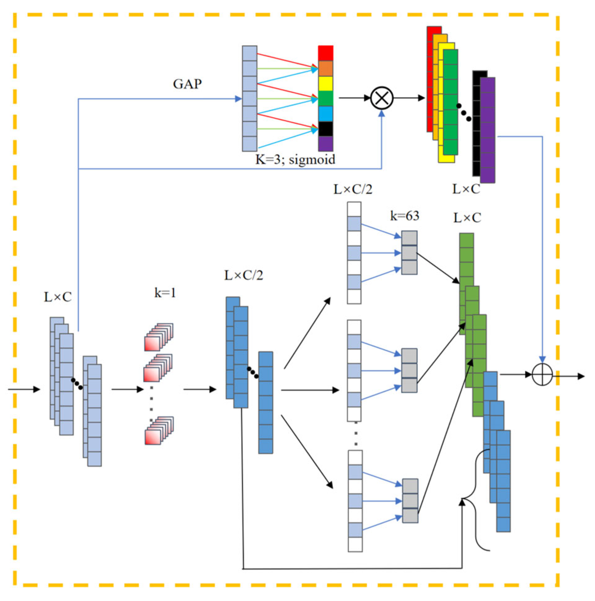
2.1. LMAF Module

This section presents the LMAF module, which integrated features extracted from multiple convolutional perspectives, including pointwise and channel-wise dilated convolutions with varying dilation rates. This design enabled the model to capture local and global signal characteristics, enhancing feature representation and noise robustness.

Dilated Convolution [32] is an extended form of the standard convolution that introduces a dilation factor. The mathematical expression is as follows:

$$y{(t)}_d={\displaystyle \sum _{k=0}^{K-1}x(t+d\times k)\cdot w(k)}$$

(1)

where d is the dilation rate, x is the input feature, w is the weight matrix of the convolution kernel, K is the size of the convolution kernel, and y is the output. When the convolution kernel size is 7, the receptive fields of the dilated convolutions with stride rates of 1, 2, and 5 are shown in Figure 1. As shown in the figure, red, yellow, and green blocks correspond to dilation rates of 1, 2, and 5 respectively, dilated convolution achieves an exponential expansion of the receptive field by adjusting the stride rate while keeping the number of convolution kernel parameters unchanged.

The combination of different dilation rates enabled the model to construct multi-scale receptive fields that capture localized and long-range signal characteristics. These diverse feature representations enhanced the model’s ability to distinguish fault patterns under varying conditions and improve its robustness to noise interference, particularly in sparsely activated regions.

Traditionally, large-kernel convolutions have rarely been used in CNNs because of their high computational cost. Ding et al. [33] proposed large-kernel channel-wise convolutions, which effectively addressed this issue. They validated the effectiveness of large-kernel channel-wise convolutions for image classification, achieving minimal increases in model parameters and FLOPs. This design further enhanced the receptive field of the convolutional layer. In addition, large-kernel per-channel dilated convolutions complemented per-point convolutions, enabling noise filtering in holes, capturing signal-induced long-range correlations, and identifying differences between channels.

The LMAF module employed pointwise convolution, large-kernel per-channel dilated convolution, and an ECA attention mechanism for multi-angle feature fusion. Figure 2 shows the LMAF structure with a dilation rate of 2.

2.1.1. Pointwise Convolution

Pointwise convolution [34] was used to extract features from different spatial locations across channels in the signal, capturing the local transient features of the signal at close range. We denoted the pointwise convolution operation using $\tau (\cdot )$. Given an input feature vector $x\in R^{L\times C_{in}}$, the output of the pointwise convolution is defined as:

$$y_i=\mathrm{BN}({\sigma }_{\mathrm{PRuLU}}(\tau {(W,x)}_i)=\mathrm{BN}({\sigma }_{\mathrm{PRuLU}}({\displaystyle \sum _k^{C_{in}}{W}_{k,i}{x}_k}))$$

(2)

where $W\in R^{C_{in}\times C_{out}}$ is the pointwise convolution kernel, L is the sequence length, C_in and C_out denote the numbers of input and output channels, ${\sigma }_{PRuLU}(\cdot )$ denotes the Parametric Rectified Linear Unit (PReLU) [35] activation function, BN stands for batch normalization, and $y_i$ is the i-th element of the output vector $y\in R^{L\times C_{out}}$ where i ∈ {1, 2, …, L} denotes the index of the sequence position.

For each layer of the convolution operation, PReLU was used as the activation function, as expressed in Equation (3).

$${\sigma }_{\mathrm{PRuLU}}(x)=\left\{\begin{array}{cc}\alpha x\hfill & x<0\\ x\hfill & x\ge 0\end{array}\right.$$

(3)

where $\alpha$ is a learnable parameter, typically a constant less than 1. PReLU enhances the model’s fitting capability without significantly increasing the number of parameters. BN was then applied to normalize the output values, and the calculation for the BN layer is shown in Equation (4).

$$n=\gamma \odot \left({\displaystyle \frac{m-{\mu }_B}{\sqrt{{\sigma }_B^2+\epsilon }}}\right)+\beta$$

(4)

where m is the input feature to the BN layer, n is the output feature of the BN layer, ${\mu }_B$ and ${\sigma }_B^2$ are the mean and variance of the current batch, respectively, and $\gamma$ and $\beta$ are the learnable parameters.

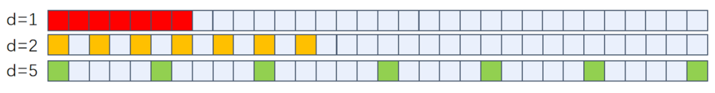
2.1.2. Channel-Wise Dilated Convolution with Large-Kernels

By adopting a large-kernel channel-wise dilated convolution, the receptive field of this convolution layer was further enhanced, complementing pointwise convolution. This enabled noise filtering in voids, capturing signal-induced long-range correlations, and identifying channel differences.

$${\widehat{y}}_{d,c}=\mathrm{BN}({\sigma }_{\mathrm{PRuLU}}({\displaystyle \sum _k^K{y}_{l+d\times k,c}\cdot W_{k,c}})$$

(5)

where $y\in R^{L\times C_{out}}$ is the input feature sequence with length L and C channels; d is the dilation rate; $W\in R^{K\times C_{out}}$ is the depthwise convolution kernel with kernel size K; and ${\widehat{y}}_{d,c}\in R^{L\times C_{out}}$ is the output feature at dilation step d for channel c where k is the kernel index (from 0 to K − 1).

2.1.3. ECA Channel Attention Module

Compared to Squeeze-and-Excitation (SE) attention [36], the ECA attention mechanism [37] has a constant number of parameters but can effectively capture the relationships between signal channels, thereby enhancing the model’s feature representation capabilities. ECA attention compresses each channel into a single feature value using global average pooling (GAP) [38], and then calculates the weights for each channel using a one-dimensional convolution layer with shared weights and a sigmoid activation function, which are then multiplied by each channel to assign weights.

$$z=\sigma (\mathrm{Conv}1D_k({\displaystyle \frac{1}{L}}{\displaystyle \sum _{l=1}^L{x}_l}))\odot x$$

(6)

where $x\in R^{L\times C_{in}}$ is the input signal with length L and C_in channels, $Conv1D_k$ denotes a 1D convolution with kernel size k and shared weights, $\sigma (\cdot )$ is the sigmoid function, $\odot$ denotes channel-wise multiplication, and $z\in R^{L\times C_{in}}$ is the output of ECA.

2.1.4. Output of the LMAF Layer

According to the model design, the output of the LMAF is as follows:

$$\widehat{z}=[y|\widehat{\mathrm{y}}]\oplus z$$

(7)

where $y\in R^{L\times C_{out}}$ is the output of the pointwise convolution module, $\widehat{y}\in R^{L\times C_{out}}$ is the output of the large-kernel channel-wise dilation convolution module, [X|Y] denotes the concatenation operation between variables X and Y, $\oplus$ denotes the channel-wise addition operation, $z\in R^{L\times C_{in}}$ is the output of ECA, C_out = C_in/2, and $\widehat{z}\in R^{L\times C_{in}}$ is the final output of the LMAF layer.

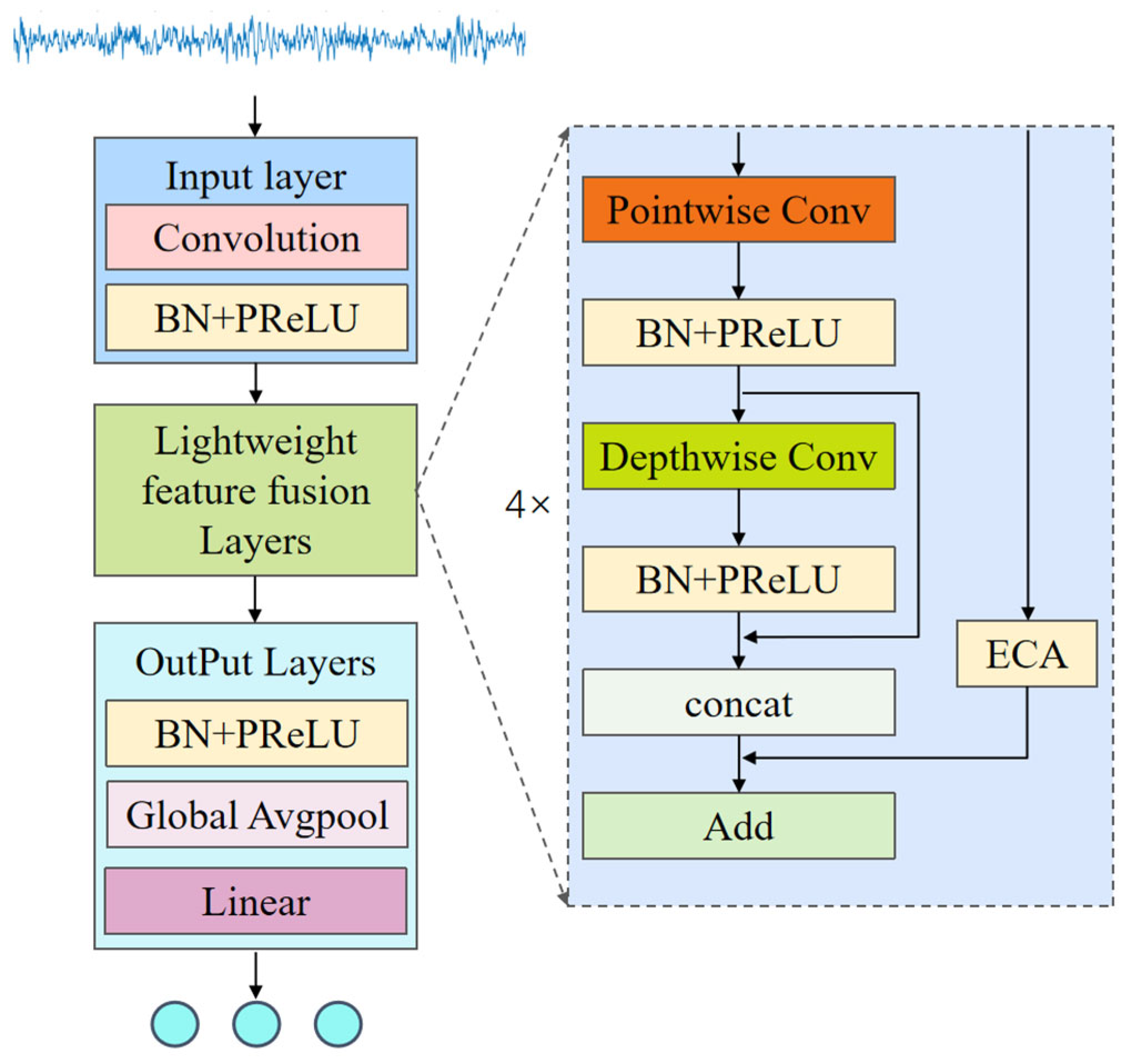
2.2. Overall Framework of LMAFCNN

Building upon the theoretical foundation presented above, we proposed the LMAFCNN, with its overall architecture illustrated in Figure 3.

The network consists of a wide-kernel convolution layer, multiple LMAF layers with different expansion rates, a GAP layer, a fully connected layer, and an output layer. The processing flow is as follows:

• Input preprocessing: First, the raw vibration signals are processed through a wide-kernel convolutional layer to achieve data compression and channel expansion, laying the foundation for subsequent multi-angle feature extraction.
• Feature learning core: Subsequently, the signals pass through multiple stacked LMAF modules, which constitute the core of the network and are responsible for learning deep features from multiple angles.
• Classification Output: Finally, the learned features are aggregated using a GAP layer, and fault diagnosis is performed using a fully connected (FC) layer and a softmax layer. The final output is a probability vector $P\in R^C$, where C denotes the number of fault categories. Each element represents the predicted probability that the input sample belongs to class i. Specifically, the final output is computed as

  $$P=\mathrm{Softmax}(\mathrm{FC}(\mathrm{GAP}({\sigma }_{\mathrm{PRuLU}}(\mathrm{BN}(\widehat{z})))))$$

  (8)

  where $\widehat{z}\in R^{L\times C_{in}}$ is the input feature map and FC is the fully connected layer projecting to the number of fault categories. Softmax converts the output of the FC layer into a probability distribution over the C fault categories, ensuring that the predicted probabilities sum to 1.

For each layer, the network uses the PReLU activation function to enhance the model’s nonlinear expression capabilities and applies BN to the inputs of each layer to prevent gradient vanishing. Owing to the large-kernel per-channel expansion convolution, which provides a strong receptive field and excellent computational efficiency, no downsampling is performed in the intermediate layers of the network, effectively avoiding the loss of fine-grained features caused by pooling operations.

Expansion convolution was used to increase the receptive field. However, a grid effect is likely to occur when multiple layers of the expansion convolution are stacked using the same dilation rate. This issue causes the convolution kernel to always act on the same input points, while data from the dilated regions are not involved in the computation for an extended period, ultimately affecting the model’s perception and the expression of fine-grained features. To effectively mitigate the grid effect, this paper adopted the Hybrid Dilated Convolution (HDC) method proposed by Panqu Wang et al. [39], which improved this by setting the dilation rate in a sawtooth-shaped cyclic structure. Specifically, this paper adopted a dilation rate stacking pattern following the sequence [1, 2, 5, 1] in the LMAF module, thereby breaking the constraint of fixed sampling points and effectively covering information from more spatial locations.

After extensive experimentation and performance evaluation of the number of feature map channels in the middle layer, the kernel size of the large-kernel channel-wise dilation convolution, the dilation rate, and the network depth within the above parameter space, a set of relatively optimal parameter combinations was determined, as detailed in

Table 1. Configuration details of the LMAFCNN.

Module	Main Branch	Sub-Branch	Convolution Kernel Size/Stride	Number of Output Channels
DownSample Conv	Conv1d	-	16/4	128
LMAF Layer1 (expansion rate = 1) LMAF Layer2 (expansion rate = 2) LMAF Layer3 (expansion rate = 5) LMAF Layer4 (expansion rate = 1)	Pointwise Conv1d	ECA	1/1	64
	Dilatation DepthwiseConv1d		63/1	64
	Concat		-	128
	Add		-	128
GAP	GAP	-	-	128
Linear	Linear	-	-	3

.

2.3. Fault Diagnosis Process Based on LMAFCNN

Bearing fault diagnosis based on the LMAFCNN model primarily consists of three key components: data preprocessing and sample construction, model construction and training, and application and analysis of the LMAFCNN fault diagnosis model. The methodological flowchart is presented in Figure 4, along with the detailed network configuration parameters in Table 1.

• Data collection and sample division: To ensure data independence and prevent information leakage, non-overlapping sliding window technology was used to divide the dataset into samples, generating mutually independent training, validation, and testing samples.
• Lightweight model design and training: The model was trained using the LMAFCNN architecture, which integrates lightweight modules, including large-kernel channel-wise dilated convolutions and ECA. The best model on the validation set was selected as the final diagnostic model.
• Fault diagnosis and result visualization: Test set data were input into the trained diagnostic model, and the diagnostic results were systematically analyzed and visualized in multiple dimensions through various technical means, such as confusion matrices and feature visualization.

3. Experimental Results and Analysis

3.1. Data Description

To validate the effectiveness of the LMAFCNN, HIT aviation interaxle bearing and PU bearing datasets were used.

3.1.1. PU Bearing Failure Dataset

The PU bearing datasets, developed by Christian Lessmeier et al. [40], contained two categories of fault data: human-induced damage and natural damage. Human-induced damage was created through artificial methods, such as electrical discharge machining (EDM), using an electric engraver, and drilling. In contrast, natural damage was obtained through accelerated life testing (primarily involving two failure modes: fatigue pitting and plastic indentation). The data collection setup is shown in Figure 5, which includes a drive motor, torque measurement shaft, bearing test module, flywheel, and load motor. The dataset used 6203-type rolling bearings, and vibration signals from the bearing housing were collected using piezoelectric accelerometers (at a sampling frequency of 64 kHz).

For the experiments, a data subset was selected under specific operating conditions (speed: 1500 rpm, load torque: 0.1 Nm, radial force: 1000 N) and divided into subsets representing artificial and natural damage. Each subset contained three sample types: inner-ring failure, outer-ring failure, and healthy state samples. The original signal was divided into non-overlapping segments of 2560 points. The labeled samples were split into an 8:1:1 ratio for training, validation, and testing. The model was trained on the training set and optimized using the validation set, and its generalization capability was assessed on the test set. The detailed data distributions of the three subsets are presented in

Table 2. Sampling details of the artificial damage dataset.

Fault Type	Label	Bearing Code	Damage Method	Damage Level	Training/Validation/Test Set
Inner ring	0	KI01	EDM	1	1440/180/180
		KI05	electric engraver	1
		KI07	electric engraver	2
Outer ring	1	KA01	EDM	1
		KA05	electric engraver	1	1440/180/180
		KA07	drilling	1
Health	2	K002	-	-	1440/180/180

and

Table 3. Sampling details of the natural damage dataset.

Fault Type	Label	Bearing Code	Damage Method	Damage Level	Training/Validation/Test Set
Inner ring	0	KI14, KI17, KI21 KI16	fatigue: potting	1	1440/180/180
			fatigue: potting	3
		KI18	fatigue: potting	2
Outer ring	1	KA04, KA22, KA16	fatigue: potting	1	1440/180/180
			fatigue: potting	2
		KA30, KA15	Plastic deform: indentations	1
Health	2	K001	-	-	1440/180/180

.

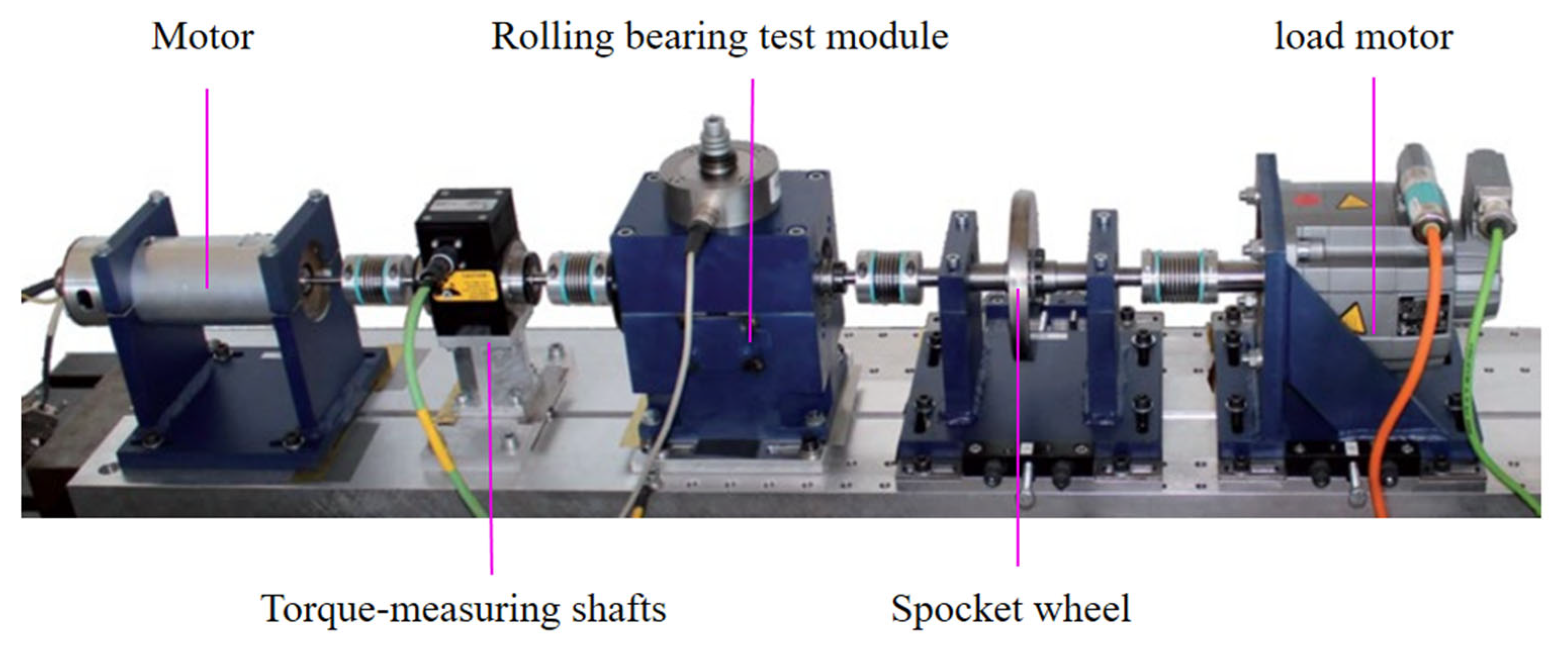
3.1.2. Harbin Institute of Technology (HIT) Aviation Intershaft Bearing Dataset

The HIT aviation intershaft bearing dataset [41] was open-sourced by Hou et al. from the Harbin Institute of Technology in 2023. The data acquisition test bench was modeled after an aviation engine, as shown in Figure 6. This dataset innovatively acquired synchronized vibration signals from both the rotor and engine casing, offering a more comprehensive characterization of complex operational conditions in practical engineering scenarios than conventional single-point measurements. The experimental data included the following three typical operating conditions: healthy state, inner-ring failure, and outer-ring failure. The sampling frequency was 25 kHz, and the rotational speed ranged from 1000 to 6000 rpm. During the data processing stage, the original 20,480-point long sequence was first divided into 1024-point non-overlapping segments. Subsequently, the dual-point signals were fused and randomly sampled to construct a balanced dataset containing 2000 samples for each category. The data were split into training, validation, and test sets in an 8:1:1 ratio, as shown in

Table 4. Sampling details of the HIT dataset.

Fault Type	Label	Fault Depth	Fault Length	Training/Validation/Test Set
Inner ring	0	0.5	0.5, 1.0	1600/200/200
Health	1	0	0	1600/200/200
Outer ring	2	0.5	0.5	1600/200/200

.

3.2. Experimental Setup

The experimental platform was equipped with an AMD Ryzen 9 7900X processor (12 cores, AMD, Santa Clara, CA, USA), 128 GB of random access memory (RAM), and an NVIDIA RTX 4090 graphics card (NVIDIA Corporation, Santa Clara, CA, USA), and the model development was implemented via PyTorch 2.6.0 (Python 3.12.7) under Windows 11 with Compute Unified Device Architecture (CUDA) 12.6 acceleration enabled throughout.

During the model training phase, the mean squared error (MSE) loss function and Adaptive Moment Estimation (Adam) optimizer were used with a fixed learning rate of 0.001. Each round of validation was set to train for 40 epochs with a batch size of 32. To enhance the reliability of the results, 10 random seeds were fixed for training, and the final performance indicators were taken as the average of the 10 independent experiments. To systematically evaluate the model’s robustness against noise, Gaussian white noise of varying intensities was added to the dataset to simulate the noise interference encountered by bearings in real-world operating environments. Gaussian white noise is commonly used in industrial fault diagnosis research to emulate sensor and acquisition noise, owing to its well-defined statistical properties and widespread applicability in evaluating model robustness under realistic interference. The model was evaluated based on accuracy, parameter count, and FLOPs.

3.3. Analysis of the Experimental Results for the PU Dataset

The noise resistance and complex condition diagnosis capabilities of LMAFCNN were evaluated by comparing them with those of WDCNN, MA1DCNN, DRSN-CW, MIXCNN2, LiconvFormer, ResNet18 [42], and MobileNetV2 [43]. We introduced Gaussian white noise with an SNR of −10, −8, −4, 0, 4, and 8 dB to simulate various noise conditions.

3.3.1. Results of Different Models

The results obtained using different methods for the different SNR levels are presented in

Table 5. The accuracy of different models on the artificial and natural damage in the PU dataset under various noise levels.

Dataset	Model	SNR (dB)
		−10	−8	−4	0	4	8	None
Artificial damage	WDCNN	65.85%	72.52%	80.09%	85.46%	88.48%	90.35%	91.63%
	MA1DCNN	71.87%	77.67%	85.33%	90.02%	93.17%	95.41%	97.63%
	DRSN_CW	65.46%	69.91%	80.04%	86.57%	90.44%	92.96%	95.41%
	ResNet18	69.78%	74.57%	82.54%	86.81%	91.07%	94.37%	97.89%
	MobileNetV2	67.46%	73.93%	82.04%	87.43%	90.83%	93.35%	96.20%
	LiConvFormer	73.85%	78.63%	85.76%	90.19%	92.61%	94.61%	97.15%
	MIXCNN2	77.35%	82.06%	88.44%	93.59%	96.65%	98.35%	99.35%
	LMAFCNN	78.91%	83.65%	90.72%	94.93%	97.74%	98.83%	99.50%
Natural injury	WDCNN	91.39%	94.89%	98.39%	99.50%	99.87%	99.98%	99.98%
	MA1DCNN	96.37%	97.70%	99.41%	99.89%	100.00%	100.00%	100.00%
	DRSN_CW	92.81%	95.76%	98.39%	99.54%	99.93%	100.00%	100.00%
	ResNet18	91.13%	93.78%	97.85%	99.57%	99.96%	100.00%	100.00%
	MobileNetV2	91.46%	94.65%	98.04%	99.63%	99.96%	100.00%	100.00%
	LiConvFormer	94.98%	97.19%	99.17%	99.91%	100.00%	100.00%	100.00%
	MIXCNN2	97.00%	98.61%	99.91%	100.00%	100.00%	100.00%	100.00%
	LMAFCNN	97.37%	98.93%	99.91%	100.00%	100.00%	100.00%	100.00%

. The line graphs in Figure 7 illustrate the fault classification accuracies of the various models on the artificial damage subset from the PU dataset across different noise environments. As shown in Table 5 and Figure 7, LMAFCNN maintained high accuracy in the presence of severe Gaussian noise. In the PU artificial damage dataset, even at SNR = −10 dB, the proposed model achieved a fault classification accuracy of 78.91%, surpassing MIXCNN2 by 1.5% and LiConvFormer by 5%. This indicated that LMAFCNN has a good resistance to noise interference and can accurately recognize bearing faults in high-noise environments.

3.3.2. Model Complexity Experiments

To verify the lightweight property of LMAFCNN, a systematic analysis was conducted in terms of the number of parameters and FLOPs.

Table 6. Comparison of the models’ lightweight performance.

Model	Number of Parameters	FLOPs
WDCNN	4.79 × 104	3.9 × 105
MA1DCNN	3.24 × 105	7.48 × 107
DRSN-CW	6.64 × 106	7.09 × 108
ResNet18	3.85 × 106	1.76 × 108
MobileNetV2	2.19 × 106	9.69 × 107
LiConvFormer	3.23 × 105	1.44 × 107
MIXCNN2	8.17 × 104	2.04 × 107
LMAFCNN	5.52 × 104	1.48 × 107

lists the parameter counts and FLOPs of each model for the input signals of length 1024.

In terms of lightweight design, as shown in Table 6, LMAFCNN contained only 5.52 × 10⁴ parameters and 1.48 × 10⁷ FLOPs, with a parameter count lower than that of all models except WDCNN, and FLOPs significantly lower than those of most models, demonstrating its outstanding model compression capability. In contrast, models such as DRSN-CW, ResNet18, and MobileNetV2, while performing adequately in terms of accuracy, had significantly higher parameter counts and computational requirements. For example, DRSN-CW had FLOPs as high as 7.09 × 10⁸, resulting in substantial computational overhead.

As such, LMAFCNN remained lightweight while maintaining powerful robustness and diagnostic capabilities.

3.3.3. Feature Visualization and Classification Performance Comparison Analysis

To further evaluate the feature extraction capabilities and fault diagnostic performance of each model, the t-SNE [44] dimensionality reduction algorithm was employed to visualize the deep features extracted by the models in two dimensions, as shown in Figure 8. Concurrently, normalized confusion matrices were used to demonstrate their diagnostic performance on the test set, with the vertical and horizontal axes representing the real and predicted labels, as shown in Figure 9. By analyzing both the separability of feature distributions and prediction accuracy, the performance differences among the models were comprehensively examined.

From Figure 8 and Figure 9, it could be observed that LMAFCNN performed best in the feature space. The feature distribution, while more dispersed than some models, appeared to show strong inter-class separation. The dispersion within a class may have suggested the model was capturing finer-grained sub-category features, which aligns with its high classification accuracy. This indicated that the model has stronger fine-grained classification capabilities and higher feature expression accuracy. Additionally, the confusion matrix results further validated this, with accuracy for all categories approaching 99% and virtually no significant misclassifications, demonstrating extremely high classification robustness. MIXCNN and MA1DCNN also exhibited good inter-class separation and intra-class aggregation capabilities, with an accuracy exceeding 98%, strong feature discriminative power, and stable classification performance. LiConvFormer had a clear feature distribution structure, with an accuracy exceeding 95%, and possessed good generalization capabilities. In contrast, ResNet18 and MobileNetV2 had blurred inter-class boundaries, and although their overall accuracy remained high, they had certain limitations in fine-grained classification. DRSN_CW exhibited a chaotic feature distribution, characterized by significant overlap between categories and relatively high misclassification rates. WDCNN performed the worst, with severe inter-class overlap and low accuracy, indicating its limited feature extraction capability.

In summary, LMAFCNN demonstrated significant advantages in fault diagnosis tasks and is suitable for high-precision diagnostic scenarios.

Furthermore, Figure 10 presents the t-SNE visualizations of the proposed LMAFCNN under different SNR conditions. The separability of deep features improved progressively as the SNR increased. Under low SNR conditions (e.g., −8 dB and −4 dB), noticeable overlap was observed between the healthy and inner ring fault samples, indicating that strong noise can obscure fault-related patterns. However, as the noise level decreased, the feature clusters become increasingly distinct, suggesting that the model can recover discriminative representations as signal quality improves. This trend is consistent with the classification accuracy, which increased steadily from 83.65% at −8 dB to 98.83% at 8 dB. These results confirmed that the proposed method maintains a certain level of diagnostic capability under heavy noise and demonstrates strong robustness as the noise diminishes.

3.4. Model Generalization Experiments

Experiments on the HIT dataset were conducted to further validate the model’s generalization. We introduced Gaussian white noise with an SNR of −10, −8, −4, 0, 4, and 8 dB to simulate various noise conditions. A comparative analysis was performed among WDCNN, DRSN-CW, MA1DCNN, ResNet18, MobileNetV2, LiConvFramer, and MIXCNN2. The detailed experimental results are presented in

Table 7. Accuracy comparison of the different models for the HIT dataset under different SNR levels.

Model	SNR (dB)
	−8	−4	0	4	8	None
WDCNN	57.98%	61.55%	66.28%	71.18%	75.93%	85.05%
MA1DCNN	55.10%	59.08%	62.98%	68.58%	71.93%	83.17%
DRSN_CW	53.15%	54.48%	56.03%	57.98%	58.67%	87.90%
ResNet18	57.22%	58.95%	60.53%	61.93%	65.03%	86.58%
MobileNetV2	57.67%	60.73%	63.05%	64.48%	66.68%	88.80%
LiConvFormer	57.70%	60.83%	64.25%	68.45%	72.00%	94.13%
MIXCNN	62.05%	65.67%	70.48%	77.62%	83.22%	94.42%
LMAFCNN	64.33%	70.82%	76.48%	81.58%	84.80%	93.12%

, and Figure 11 provides a clustered bar chart visualization of these results.

As shown in Figure 11 and Table 7, the results demonstrated that the proposed LMAFCNN consistently outperformed the other models in low SNR environments. Specifically, it achieved an accuracy of 64.33% at −8 dB and 70.82% at −4 dB, significantly surpassing traditional models such as WDCNN, ResNet18, and MA1DCNN, whose performance drops markedly under strong noise interference.

Although MIXCNN achieved the highest accuracy of 94.42% under clean (noiseless) conditions, its performance under high-noise levels was slightly lower than that of LMAFCNN. Notably, LMAFCNN maintained high and stable accuracy across all noise levels, reaching 84.80% at 8 dB and 93.12% without noise, indicating excellent generalization and noise robustness. Overall, the results confirmed that LMAFCNN achieved a better trade-off between accuracy and robustness, making it well-suited for practical bearing fault diagnosis in noisy industrial environments.

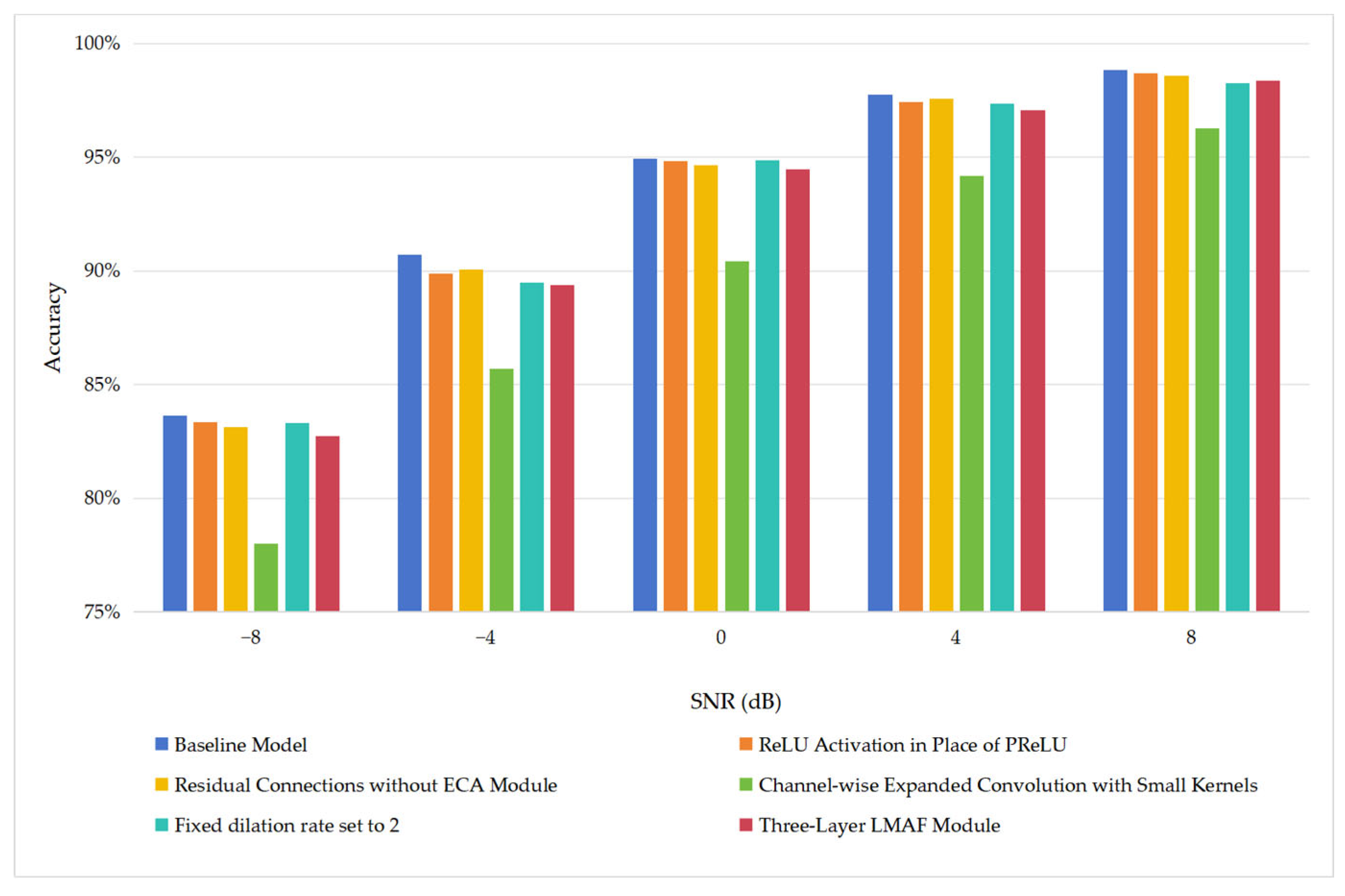
3.5. Ablation Experiment

To validate the role of each module in LMAFCNN, ablation experiments were designed to investigate the contribution of key modules in the LMAFCNN model under different SNR levels, including the following: (1) replacing PReLU with ReLU, (2) removing the ECA attention mechanism while retaining residual connections, (3) adopting a three-layer LMAF module, (4) all LMAF layers using a fixed dilation rate of 2, and (5) removing the large-kernel channel-by-channel expanded convolution. The experimental results based on the PU artificial dataset are presented in

Table 8. Ablation experiment results under different SNR levels.

Model	SNR
	−8 dB	−4 dB	0 dB	4 dB	8 dB
Baseline Model	83.65%	90.72%	94.93%	97.74%	98.83%
ReLU Activation in Place of PReLU	83.35%	89.89%	94.81%	97.41%	98.70%
Residual Connections without ECA Module	83.13%	90.06%	94.65%	97.56%	98.57%
Channel-wise Expanded Convolution with Small Kernels	78.00%	85.70%	90.43%	94.17%	96.28%
Fixed dilation rate set to 2	83.30%	89.50%	94.85%	97.35%	98.26%
Three-Layer LMAF Module	82.74%	89.37%	94.46%	97.06%	98.37%

and Figure 12.

The results showed that the baseline model with the complete structure performed best across all SNR levels, indicating that each module plays a crucial role in enhancing the model’s robustness and diagnostic accuracy. When large-kernel channel-wise dilated convolutions were removed, the model performance degraded most significantly, dropping to 78.00% at −8 dB, indicating that long-range correlation features play a critical role in bearing fault diagnosis tasks. Large-kernel channel-wise dilated convolutions effectively capture these dependencies by expanding the receptive field, while their dilation structure contributes strong noise-suppression capabilities. Together, these properties significantly enhanced the model’s ability to maintain stable performance under noisy conditions.

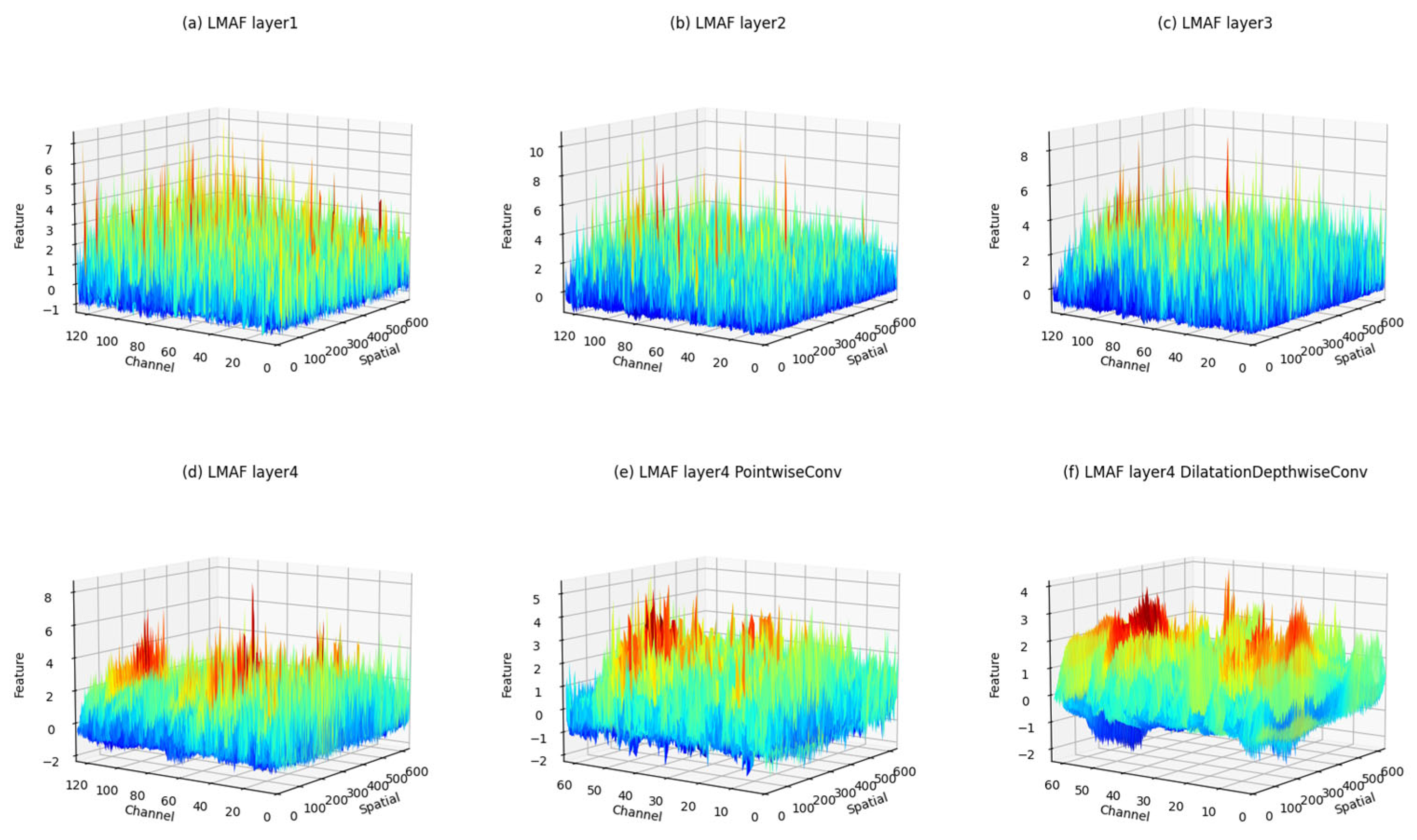
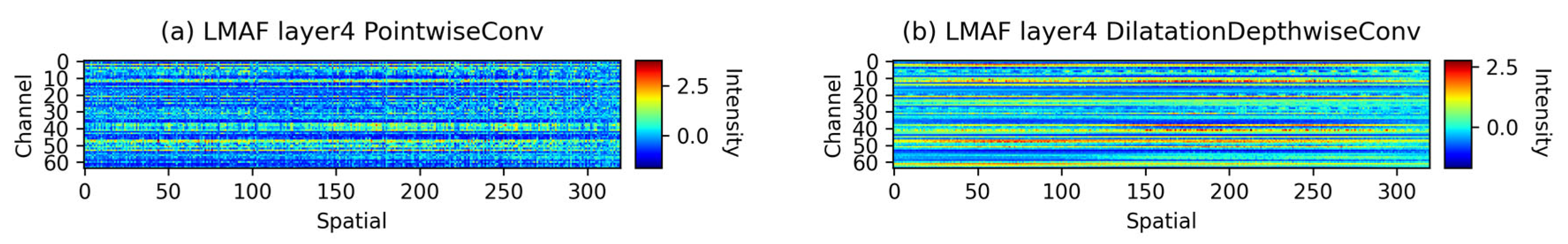
3.6. Model Interpretability Analysis

Based on the experimental results, the LMAFCNN model demonstrated outstanding performance in terms of noise resistance, versatility, generalization ability, and lightweight design. Its feature extraction capabilities were further explored, revealing that the effectiveness of LMAFCNN stemmed from a multi-angle feature fusion mechanism.

Owing to the hierarchical structure of convolutional neural networks, data continuously acquire new features as they pass through the successive layers of LMAFCNN modules, ultimately enabling different categories to gradually separate in the feature space, thereby achieving the accurate classification of various categories by the fully connected layer. Figure 13 illustrates the feature attention mechanism of the core layers of the model in both the channel and spatial dimensions. This three-dimensional diagram was generated based on the inference process of the LMAFCNN model, which was trained on the noise-free HIT dataset and evaluated during testing, clearly reflecting the distribution of response intensities across different channels and spatial positions in the output feature maps of each layer.

Noise Suppression and Feature Focusing Process: In the initial LMAF1 stage, due to noise interference, the distribution of feature responses was relatively uniform and contained a large number of zero values. As the network depth increased (Figure 13d), the model gradually learned richer and more discriminative features. By the final LMAF layer, the model exhibited clear feature selectivity: responses in key channels and spatial locations were significantly enhanced with high response values, while non-key regions were strongly suppressed with response values approaching zero.

Multi-scale feature capture capability: LMAFCNN effectively achieved the joint learning of local near-distance features and global long-range correlation features through the synergistic effect of pointwise convolution and large-kernel channel-wise dilation convolution. As shown in Figure 13e,f and the heatmap in Figure 14 (this heatmap scales the number of channels and data length by a factor of 2, ultimately displaying a feature map with 64 channels and a length of 320 points), the feature maps obtained after the data passes through the different convolution operations in LMAF are demonstrated..

As shown in Figure 14, the high-response regions generated by pointwise convolution were concentrated and had a small coverage area, primarily focusing on local features. In contrast, the large-kernel channel-wise dilation convolution exhibited widely distributed response regions, nearly covering the entire data length, reflecting its ability to perceive long-range associated features. Additionally, as shown in Figure 13, the model demonstrated varying degrees of attention to different channels, further validating its channel-selective feature extraction capability.

The above analysis and feature visualization results verified that the core advantage of LMAFCNN stems from its multi-angle feature learning and fusion mechanism. This mechanism synergistically fuses local transient features extracted by pointwise convolution with long-range dependency features captured by large-kernel dilated convolution, demonstrating the effectiveness and interpretability of LMAFCNN. This fusion enabled the model to handle a broader range of complex bearing fault diagnosis scenarios.

4. Conclusions

To address the challenges of excessive model parameters and poor noise resistance in traditional CNNs for bearing fault diagnosis, this study introduced LMAFCNN, which leverages lightweight multi-angle feature fusion for improved robustness. The model extracts features through the LMAF module at multiple levels, uses pointwise convolution to capture features in different spatial and short-distance domains, and combines large-kernel channel expansion convolution to obtain cross-channel and long-distance features. Additionally, a sawtooth-shaped dilation rate strategy was introduced to enhance the comprehensive perception of long-range features, and the ECA attention mechanism was integrated to selectively enhance the response of critical channels.

The accuracies on the PU artificial damage, PU natural damage bearing, and HIT datasets were 99.5%, 100%, and 93.12%, respectively. At low SNR levels, LMAFCNN demonstrated significantly superior performance compared to existing methods, such as WDCNN, MA1DCNN, DRSN-CW, MIXCNN2, LiConvFormer, and ResNet18. The model contains approximately 55.2 K parameters and has a computational cost of 14.8 MFLOPs, fully demonstrating its lightweight architecture and computational efficiency. LMAFCNN effectively extracted and fused multi-view features, significantly improving classification accuracy in noisy environments, and provides an effective solution for bearing fault diagnosis under complex operating conditions. The proposed LMAFCNN method achieved a novel balance between diagnostic performance and computational efficiency. In future work, we aim to address several limitations: (1) explore diagnostic strategies under class-imbalanced data conditions, which are common in real-world applications; (2) validate the model’s robustness in actual industrial noise environments beyond Gaussian noise; and (3) extend the framework to incorporate multi-sensor data fusion for the improved diagnosis of complex compound faults.

References

1. Kumar, S.; Mukherjee, D.; Guchhait, P.K.; Banerjee, R.; Srivastava, A.K.; Vishwakarma, D.N.; Saket, R.K. A Comprehensive Review of Condition Based Prognostic Maintenance (CBPM) for Induction Motor. IEEE Access 2019, 7, 90690–90704. [Google Scholar] [CrossRef]
2. Wei, Z.; Xu, Y.; Nolan, J.P. An alternative bearing fault detection strategy for vibrating screen bearings. J. Vib. Control 2023, 30, 4304–4316. [Google Scholar] [CrossRef]
3. Barai, V.; Ramteke, S.M.; Dhanalkotwar, V.; Nagmote, Y.; Shende, S.; Deshmukh, D. Bearing fault diagnosis using signal processing and machine learning techniques: A review. In Proceedings of the IOP Conference Series: Materials Science and Engineering, Nagpur, India, 26–28 May 2022; p. 012034. [Google Scholar]
4. Jiang, D.; He, C.; Chen, Z.; Zhao, J. Are Novel Deep Learning Methods Effective for Fault Diagnosis? IEEE Trans. Reliab. 2024, 1–15. [Google Scholar] [CrossRef]
5. Zhao, J.; Wang, W.; Huang, J.; Ma, X. A comprehensive review of deep learning-based fault diagnosis approaches for rolling bearings: Advancements and challenges. AIP Adv. 2025, 15, 020702. [Google Scholar] [CrossRef]
6. Zhu, Z.; Lei, Y.; Qi, G.; Chai, Y.; Mazur, N.; An, Y.; Huang, X. A review of the application of deep learning in intelligent fault diagnosis of rotating machinery. Measurement 2023, 206, 112346. [Google Scholar] [CrossRef]
7. Ko, J.H.; Yin, C. A review of artificial intelligence application for machining surface quality prediction: From key factors to model development. J. Intell. Manuf. 2025. [Google Scholar] [CrossRef]
8. Wu, M.; Arshad, M.H.; Saxena, K.K.; Qian, J.; Reynaerts, D. Profile prediction in ECM using machine learning. Procedia CIRP 2022, 113, 410–416. [Google Scholar] [CrossRef]
9. Chung, J.; Shen, B.; Kong, Z.J. Anomaly detection in additive manufacturing processes using supervised classification with imbalanced sensor data based on generative adversarial network. J. Intell. Manuf. 2024, 35, 2387–2406. [Google Scholar] [CrossRef]
10. Gong, L.; Pang, C.; Wang, G.; Shi, N. Lightweight Bearing Fault Diagnosis Method Based on Improved Residual Network. Electronics 2024, 13, 3749. [Google Scholar] [CrossRef]
11. Zhang, G.; Xu, J.; Huang, X.; Li, Z. A Novel Two-Dimensional Quad-Stable Stochastic Resonance System for Bearing Fault Detection. Fluct. Noise Lett. 2023, 23, 2450017. [Google Scholar] [CrossRef]
12. Gong, W.; Wang, Y.; Zhang, M.; Mihankhah, E.; Chen, H.; Wang, D. A Fast Anomaly Diagnosis Approach Based on Modified CNN and Multisensor Data Fusion. IEEE Trans. Ind. Electron. 2022, 69, 13636–13646. [Google Scholar] [CrossRef]
13. Li, X.; Chen, Y.; Liu, Y. A novel convolutional neural network with global perception for bearing fault diagnosis. Eng. Appl. Artif. Intell. 2025, 143, 109986. [Google Scholar] [CrossRef]
14. Zheng, X.; Hu, Q.; Li, C.; Zhao, S. An Enhanced Dual-Channel-Omni-Scale 1DCNN for Fault Diagnosis. In Proceedings of the Chinese Conference on Pattern Recognition and Computer Vision (PRCV), Urumqi, China, 18–20 October 2024; pp. 152–166. [Google Scholar]
15. Janssens, O.; Slavkovikj, V.; Vervisch, B.; Stockman, K.; Loccufier, M.; Verstockt, S.; Van de Walle, R.; Van Hoecke, S. Convolutional Neural Network Based Fault Detection for Rotating Machinery. J. Sound Vib. 2016, 377, 331–345. [Google Scholar] [CrossRef]
16. Zhang, W.; Peng, G.; Li, C.; Chen, Y.; Zhang, Z. A New Deep Learning Model for Fault Diagnosis with Good Anti-Noise and Domain Adaptation Ability on Raw Vibration Signals. Sensors 2017, 17, 425. [Google Scholar] [CrossRef]
17. Zhao, M.; Zhong, S.; Fu, X.; Tang, B.; Pecht, M. Deep Residual Shrinkage Networks for Fault Diagnosis. IEEE Trans. Ind. Inf. 2020, 16, 4681–4690. [Google Scholar] [CrossRef]
18. Wang, C.; Li, X.; Yuan, P.; Su, K.; Xie, Z.; Wang, J. An integrated approach for mechanical fault diagnosis using maximum mean square discrepancy representation and CNN-based mixed information fusion. Struct. Health Monit. 2024, 14759217241279996. [Google Scholar] [CrossRef]
19. Wang, H.; Liu, Z.; Peng, D.; Qin, Y. Understanding and Learning Discriminant Features based on Multiattention 1DCNN for Wheelset Bearing Fault Diagnosis. IEEE Trans. Ind. Inf. 2020, 16, 5735–5745. [Google Scholar] [CrossRef]
20. Fang, H.; Deng, J.; Zhao, B.; Shi, Y.; Zhou, J.; Shao, S. LEFE-Net: A Lightweight Efficient Feature Extraction Network with Strong Robustness for Bearing Fault Diagnosis. IEEE Trans. Instrum. Meas. 2021, 70, 1–11. [Google Scholar] [CrossRef]
21. Zhao, Z.; Jiao, Y. A Fault Diagnosis Method for Rotating Machinery Based on CNN with Mixed Information. IEEE Trans. Ind. Inf. 2023, 19, 9091–9101. [Google Scholar] [CrossRef]
22. Jin, T.; Yan, C.; Chen, C.; Yang, Z.; Tian, H.; Guo, J. New domain adaptation method in shallow and deep layers of the CNN for bearing fault diagnosis under different working conditions. Int. J. Adv. Manuf. Technol. 2023, 124, 3701–3712. [Google Scholar] [CrossRef]
23. Li, S.; Jiang, Q.; Xu, Y.; Feng, K.; Wang, Y.; Sun, B.; Yan, X.; Sheng, X.; Zhang, K.; Ni, Q. Digital twin-driven focal modulation-based convolutional network for intelligent fault diagnosis. Reliab. Eng. Syst. Saf. 2023, 240, 109590. [Google Scholar] [CrossRef]
24. Wang, H.; Zhu, H.; Li, H. A rotating machinery fault diagnosis method based on multi-sensor fusion and ECA-CNN. IEEE Access 2023, 11, 106443–106455. [Google Scholar] [CrossRef]
25. Chen, G.; Song, W.; Shao, W.; Sun, H.; Qing, X. Damage presence, localization and quantification of aircraft structure based on end-to-end deep learning framework. IEEE Trans. Instrum. Meas. 2025, 74, 1–15. [Google Scholar] [CrossRef]
26. Hu, B.; Liu, J.; Xu, Y. A novel multi-scale convolutional neural network incorporating multiple attention mechanisms for bearing fault diagnosis. Measurement 2025, 242, 115927. [Google Scholar] [CrossRef]
27. Yan, H.; Si, X.; Liang, J.; Duan, J.; Shi, T. Unsupervised Learning for Machinery Adaptive Fault Detection Using Wide-Deep Convolutional Autoencoder with Kernelized Attention Mechanism. Sensors 2024, 24, 8053. [Google Scholar] [CrossRef]
28. Yan, S.; Shao, H.; Wang, J.; Zheng, X.; Liu, B. LiConvFormer: A lightweight fault diagnosis framework using separable multiscale convolution and broadcast self-attention. Expert Syst. Appl. 2024, 237, 121338. [Google Scholar] [CrossRef]
29. Li, X.; Wang, Y.; Yao, J.; Li, M.; Gao, Z. Multi-sensor fusion fault diagnosis method of wind turbine bearing based on adaptive convergent viewable neural networks. Reliab. Eng. Syst. Saf. 2024, 245, 109980. [Google Scholar] [CrossRef]
30. Xu, H.; Wang, X.; Huang, J.; Zhang, F.; Chu, F. Semi-supervised multi-sensor information fusion tailored graph embedded low-rank tensor learning machine under extremely low labeled rate. Inf. Fusion 2024, 105, 102222. [Google Scholar] [CrossRef]
31. Mitra, S.; Koley, C. Real-time robust bearing fault detection using scattergram-driven hybrid CNN-SVM. Electr. Eng. 2024, 106, 3615–3625. [Google Scholar] [CrossRef]
32. Yu, F.; Koltun, V. Multi-scale context aggregation by dilated convolutions. arXiv 2015, arXiv:1511.07122. [Google Scholar]
33. Ding, X.; Zhang, X.; Han, J.; Ding, G. Scaling up your kernels to 31x31: Revisiting large kernel design in cnns. In Proceedings of the IEEE/CVF Conference on Computer Vision and Pattern Recognition (CVPR), New Orleans, LA, USA, 18–24 June 2022; pp. 11963–11975. [Google Scholar]
34. Chollet, F. Xception: Deep learning with depthwise separable convolutions. In Proceedings of the IEEE Conference on Computer Vision and Pattern Recognition, Honolulu, HI, USA, 21–26 July 2017; pp. 1251–1258. [Google Scholar]
35. He, K.; Zhang, X.; Ren, S.; Sun, J. Delving deep into rectifiers: Surpassing human-level performance on imagenet classification. In Proceedings of the IEEE International Conference on Computer Vision, Santiago, Chile, 7–13 December 2015; pp. 1026–1034. [Google Scholar]
36. Hu, J.; Shen, L.; Sun, G. Squeeze-and-excitation networks. In Proceedings of the IEEE Conference on Computer Vision and Pattern Recognition, Salt Lake City, UT, USA, 18–23 June 2018; pp. 7132–7141. [Google Scholar]
37. Wang, Q.; Wu, B.; Zhu, P.; Li, P.; Zuo, W.; Hu, Q. ECA-Net: Efficient channel attention for deep convolutional neural networks. In Proceedings of the IEEE/CVF Conference on Computer Vision and Pattern Recognition, Seattle, WA, USA, 13–19 June 2020; pp. 11534–11542. [Google Scholar]
38. Lin, M.; Chen, Q.; Yan, S. Network in network. arXiv 2013, arXiv:1312.4400. [Google Scholar]
39. Wang, P.; Chen, P.; Yuan, Y.; Liu, D.; Huang, Z.; Hou, X.; Cottrell, G. Understanding Convolution for Semantic Segmentation. In Proceedings of the IEEE Winter Conference on Applications of Computer Vision (WACV), Lake Tahoe, NV, USA, 12–15 March 2018; pp. 1451–1460. [Google Scholar]
40. Lessmeier, C.; Kimotho, J.K.; Zimmer, D.; Sextro, W. Condition monitoring of bearing damage in electromechanical drive systems by using motor current signals of electric motors: A benchmark data set for data-driven classification. In Proceedings of the PHM Society European Conference, Bilbao, Spain, 5–8 July 2016. [Google Scholar]
41. Hou, L.; Yi, H.; Jin, Y.; Gui, M.; Sui, L.; Zhang, J.; Chen, Y. Inter-shaft bearing fault diagnosis based on aero-engine system: A benchmarking dataset study. J. Dyn. Monit. Diagn. 2023, 2, 228–242. [Google Scholar] [CrossRef]
42. He, K.; Zhang, X.; Ren, S.; Sun, J. Deep residual learning for image recognition. In Proceedings of the IEEE Conference on Computer Vision and Pattern Recognition, Las Vegas, NV, USA, 27–30 June 2016; pp. 770–778. [Google Scholar]
43. Sandler, M.; Howard, A.; Zhu, M.; Zhmoginov, A.; Chen, L.-C. Mobilenetv2: Inverted residuals and linear bottlenecks. In Proceedings of the IEEE Conference on Computer Vision and Pattern Recognition, Salt Lake City, UT, USA, 18–23 June 2018; pp. 4510–4520. [Google Scholar]
44. Van der Maaten, L.; Hinton, G. Visualizing data using t-SNE. J. Mach. Learn. Res. 2008, 9, 2579–2605. [Google Scholar]
Figure 1. Receptive fields of cavity convolutions with different expansion rates.
Electronics 14 02774 g001
Figure 2. Structural diagram of the LMAF module with a dilation rate of 2.
Electronics 14 02774 g002
Figure 3. Network architecture of the LMAFCNN model.
Electronics 14 02774 g003
Figure 4. Fault diagnosis process based on the LMAFCNN framework.
Electronics 14 02774 g004
Figure 5. Test bench for the PU bearing dataset.
Electronics 14 02774 g005
Figure 6. Test bench for HIT dataset signal acquisition.
Electronics 14 02774 g006
Figure 7. Comparison of the models for the PU artificial damage dataset under various noise levels.
Electronics 14 02774 g007
Figure 8. t-SNE visualization of feature maps from different methods.
Electronics 14 02774 g008
Figure 9. Confusion matrices of the different methods. The vertical axis represents the real labels, and the horizontal axis represents the predicted labels. The values indicate the classification accuracy (%) for each class.
Electronics 14 02774 g009
Figure 10. t-SNE visualization of feature maps extracted by the proposed method under different SNR conditions.
Electronics 14 02774 g010
Figure 11. Clustered bar chart comparing model accuracy under different SNR levels on the HIT dataset.
Electronics 14 02774 g011
Figure 12. Line plots of ablation experiment results under varying SNR levels.
Electronics 14 02774 g012
Figure 13. The 3D visualization of feature maps after selected layers in LMAFCNN.
Electronics 14 02774 g013
Figure 14. Heatmap of feature maps after pointwise convolution and channel-wise large-kernel expansion convolution.
Electronics 14 02774 g014