A Comparative Study on Machine Learning Methods for EEG-Based Human Emotion Recognition

Abstract

Electroencephalogram (EEG) signals provide a direct and non-invasive means of interpreting brain activity and are increasingly becoming valuable in embedded emotion-aware systems, particularly for applications in healthcare, wearable electronics, and human–machine interactions. Among various EEG-based emotion recognition techniques, deep learning methods have demonstrated superior performance compared to traditional approaches. This advantage stems from their ability to extract complex features—such as spectral–spatial connectivity, temporal dynamics, and non-linear patterns—from raw EEG data, leading to a more accurate and robust representation of emotional states and better adaptation to diverse data characteristics. This study explores and compares deep and shallow neural networks for human emotion recognition from raw EEG data, with the goal of enabling real-time processing in embedded and edge-deployable systems. Deep learning models—specifically convolutional neural networks (CNNs) and recurrent neural networks (RNNs)—have been benchmarked against traditional approaches such as the multi-layer perceptron (MLP), support vector machine (SVM), and k-nearest neighbors (kNN) algorithms. This comparative study investigates the effectiveness of deep learning techniques in EEG-based emotion recognition by classifying emotions into four categories based on the valence–arousal plane: high arousal, positive valence (HAPV); low arousal, positive valence (LAPV); high arousal, negative valence (HANV); and low arousal, negative valence (LANV). Evaluations were conducted using the DEAP dataset. The results indicate that both the CNN and RNN-STM models have a high classification performance in EEG-based emotion recognition, with an average accuracy of 90.13% and 93.36%, respectively, significantly outperforming shallow algorithms (MLP, SVM, kNN).

1. Introduction

Human emotions play a significant role in cognitive ability, specifically in perception, human interaction, decision-making, and human intelligence. Emotion recognition is crucial and has several applications in areas such medicine, industry, educational systems, and the military [1]. In fact, emotion recognition is a way of understanding humans’ emotional status. Emotion recognition analysis benefits from the progress of cognitive science, psychology, computer science, and modern neuroscience [2].

Emotion detection can be conducted using both physiological and non-physiological signals. Non-physiological signals include speech, facial expression, and posture. In contrast, some wearable devices can detect physiological signals, such as an electromyogram (EMG), an electroencephalogram (EEG), an electrocardiogram (ECG), skin response, and blood volume/pressure [3]. Recent advances also include wearable devices such as smart wristbands that continuously monitor respiratory rate, heart rate, and blood pressure. These systems often employ optical sensors (e.g., photoplethysmography (PPG)) and integrate machine learning algorithms to extract and classify time- and frequency-domain features from raw signals. For instance, in [4], a wearable photonic wristband was developed and achieved over 98% accuracy in biometric identification using power spectral density (PSD)-based features extracted from PPG signals. Similarly, in [5], the authors demonstrated a multi-modal smart band that fused PPG and accelerometer data with deep learning for real-time respiratory monitoring during daily activities. These technologies highlight the potential of combining physiological sensing with machine learning for both health monitoring and biometric identification in real-world settings. Non-physiological signals are not reliable indicators of emotion, as they may not arise because of emotional response or may be intentionally deceptive. In contrast, physiological signals demonstrate a higher accuracy since they cannot be controlled by the user. EEG-based emotion recognition methods provide a precise assessment of emotions among different methods of physiological brain records, enabling their application in diverse fields, including affective computing, human–computer interactions, and healthcare diagnostics [6].

In recent years, researchers have introduced several approaches for emotion recognition based on EEG signals. The complexity of EEG signals, namely spatial, spectral, non-linear dynamics, and temporal features, necessitates the development of deep networks for accurate interpretation. Notably, the application of deep learning (DL) algorithms and machine learning (ML) algorithms has revolutionized this field, marking a significant shift in the principle of emotion recognition. Traditional ML approaches, such as the k-nearest neighbors (kNN) and support vector machine (SVM) methods, have limitations, including the complex formulas required for feature extraction and their susceptibility to electromyography artifacts [7]. To overcome these challenges, deep learning methods are employed, as they excel in handling both structured and unstructured data. This is particularly important as data volume increases, ensuring superior performance compared to traditional ML algorithms [8]. Indeed, the final goal is to develop a low-complexity emotion recognition system that can provide a high classification accuracy. Additionally, valence and arousal can be considered as two essential dimensions of human emotions that have been utilized to describe and classify them. Arousal shows the level or intensity of activation associated with that emotion (e.g., anxiety or calmness), whereas valence specifies whether an emotion is negative or positive (e.g., sadness or happiness). A CNN model is developed in [9] to detect emotional valence and analyze different emotions using EEG signals. In [10], deep belief networks (DBNs) are utilized to study important EEG channels and frequency bands for emotion recognition. In addition, DBN and CNN networks are used to classify the valence of emotion in [11] and [12], respectively. Unsupervised DL methods are also used to extract features from EEG signals automatically; for instance, autoencoder models are employed in [13] to generate EEG representations. A dynamical graph convolutional neural network (DGCNN) is developed in [14], while a multimodal residual LSTM (MMResLSTM) network is developed in [15] for EEG emotion classification. Further, RNN architectures with different specifications are developed for emotion classification [16]. As EEG signals exhibit a sequential nature, RNNs are expected to offer a unique perspective in emotion recognition tasks, complementing the strengths of other DL architectures such as CNNs and DBNs. The significant contributions of this study include the following:

• Presentation of efficient techniques for analyzing and visualizing EEG datasets.
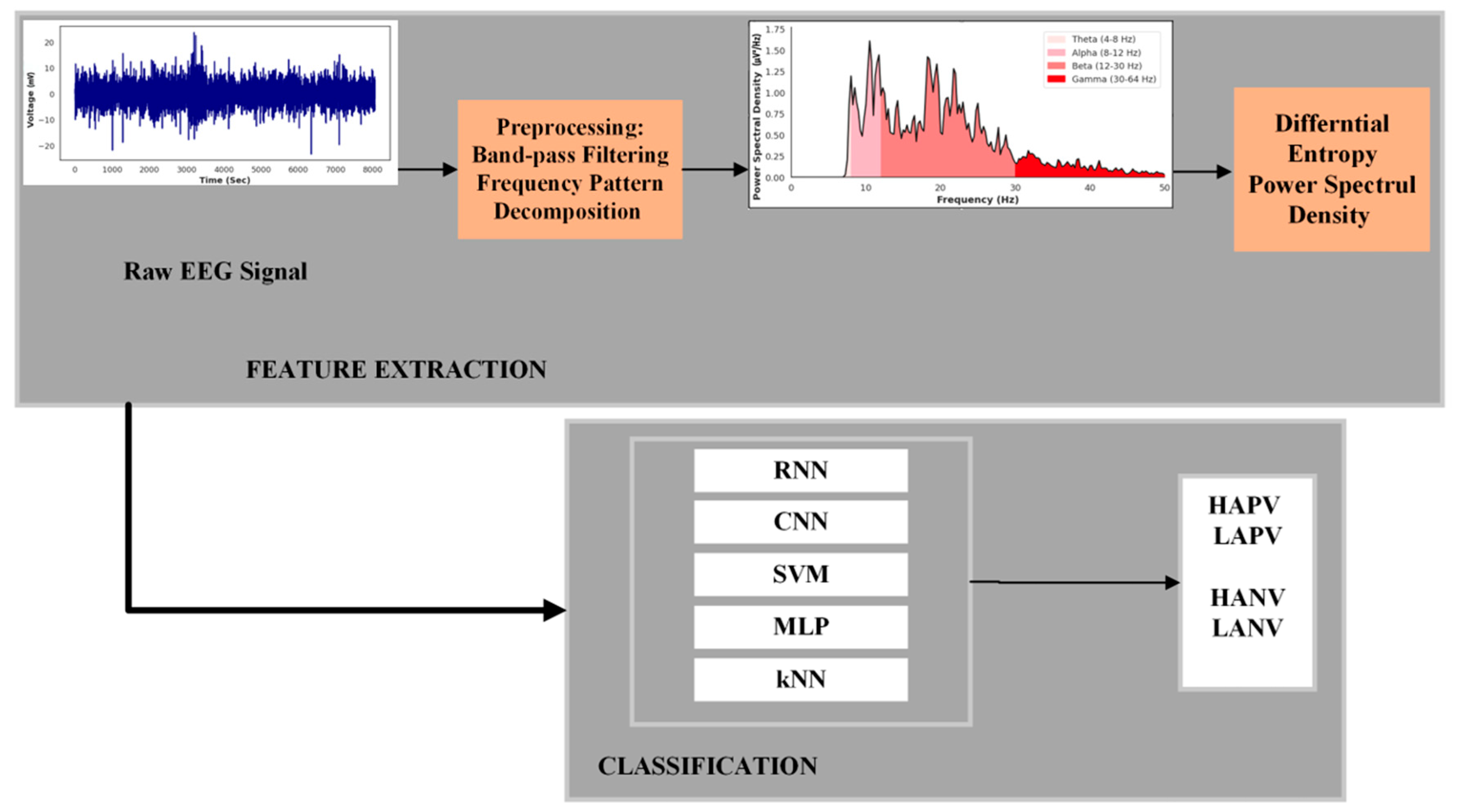
• A detailed methodology for utilizing key EEG features such as power spectral density (PSD) and differential entropy (DE).
• An effective approach for integrating feature selection, feature extraction, and classification algorithms.
• A comparative analysis of shallow and deep networks for EEG-based emotion classification.

This study integrates both PSD and DE feature extraction methods, rather than relying on a single technique [17]. In addition, the inherent differences between shallow and deep learning models [18], are examined to elucidate the observed performance discrepancies. Specifically, the classification performance of kNN, MLP, and SVM as shallow algorithms, and the CNN and RNN as deep algorithms, is evaluated to guide researchers in selecting the most effective algorithm based on the desired accuracy and application context. The following sections include a detailed explanation of the proposed approach and demonstration of the results, and concludes with a summary of the research.

2. Materials and Methods

2.1. Emotional EEG Dataset

In this paper, the database for emotion analysis using physiological signals (DEAP), developed by Koelstra and colleagues [19], is utilized as a multimodal dataset. This dataset contains peripheral physiological signals with eight channels, and EEG signals with 32 channels. To collect the data, 32 healthy volunteers were asked to watch 40 one-minute-long emotional music videos while recording their signals. Each volunteer rated the level of valence, arousal, dominance, and liking for 40 videos, ranging from 1 to 9. The data for each trial consisted of 3 s baseline data and 60 serial datasets. The EEG signals were recorded at a sampling rate of 512 Hz and then down-sampled to 128 Hz (

Table 1. DEAP dataset structure.

Total
Subjects	EEG Channels	Videos	Sampling rate	Label	Scale range
32	32	40	128 Hz	Valence and arousal	Continuous scale of 1–9
The format of EEG data for one subject (preprocessed version)
Array	Dimension		Content
Labels	2 × 40		Label (valence, arousal) × trial/video
Data	32 × 8064 × 40		Channels × data × trial/video

). In this study, only EEG signals were used, with a focus on four specific classes that differentiate between high and low valence levels and high and low arousal levels. The classification of the emotional states is conducted at the level of each time step in the EEG recordings. In order to compare the valence and arousal ratings within each of the four classes effectively and visualize the distribution of data, box plots have been constructed and are displayed in Figure 1a,b. This visualization method allows us to compare the four class distributions across the dataset, as well as analyze the dataset’s variability and central tendency (median), recognize outliers, and comprehend the range of data within each class. In fact, the level of emotional states represented by the different classes is clarified, facilitating a comprehensive analysis of the data. As is shown in the box plots for each class, low levels (low valance/arousal) are represented by values between 0 and 5, while high levels (high valence/arousal) range from 5 to 9. Also, it can be observed that there are no outliers present within the dataset. The histogram in Figure 1 shows the distribution of samples across the four emotional groups.

2.2. Preprocessing

Electroencephalography measures the electrical activity in the cerebral cortex using electrodes placed on the scalp. For emotion recognition, spatial features from the raw EEG data are crucial, focusing on signal variations (covariance) and similarities (correlation) across different scalp locations. In addition to spatial features, time-domain and frequency-domain features are essential for detecting correlations between brain activity and emotions. Time-domain analysis focuses on measuring signal characteristics over time, such as the amplitude, mean, standard deviation, latency, and baseline offset. In contrast, frequency-domain analysis transforms the EEG signal into its frequency components using techniques such as the Fourier transform. This enables the identification of frequency-related patterns that are linked to emotional states.

The quality and reliability of EEG signals can be significantly impacted by a variety of external and internal artifacts. Therefore, preprocessing is an essential step in the development of recognition algorithms, particularly those aimed at emotion recognition. Depending on the study requirements, preprocessing techniques can be divided into two categories, namely high- and low-level preprocessing [20].

Low-level preprocessing is extensively employed to remove different types of noise, such as muscle activity, electrical interference, and movement artifacts. According to the authors in [20], noise reduction, normalization, windowing, and baseline correction are among the most significant low-level preprocessing techniques for EEG signals. High-level preprocessing methods, also known as advanced preprocessing, are required for interpreting EEG signals, decomposing them into different frequency bands, and extracting meaningful features such as DE, PSD, event-related potentials (ERPs), and connectivity measures [21]. These methods include empirical mode decomposition, wavelet transform, short time, and fast Fourier transform. For instance, PSD shows the distribution of signal power across various frequency ranges, while DE quantifies the uncertainty or complexity of the signal’s distribution. Incorporating these features alongside ERPs and connectivity measures improves the ability to distinguish between different patterns in the analysis. In this study, the preprocessed version of the DEAP dataset was used, where EEG signals were down-sampled from 512 Hz to 128 Hz. Standard preprocessing was applied, including a notch filter to eliminate powerline interference (50/60 Hz) and a bandpass filter (4–45 Hz) to retain frequency components relevant to emotion recognition. Baseline correction and normalization were performed to reduce inter-subject variability. Artifact-prone segments, such as those affected by eye or muscle movements, were minimized using standard procedures provided in the dataset’s preprocessing pipeline. After filtering, the Gaussianity of the EEG signals was evaluated using the Kolmogorov–Smirnov test. Features were then extracted from EEG sub-bands in the form of PSD and DE, which were subsequently used as inputs to the deep learning models.

2.3. Frequency Pattern Decomposition and Feature Extraction

2.3.1. Differential Entropy

Entropy measures how much information is required to talk about randomness in a set of continuous random variables and can be used for feature extraction. Differential entropy refers to a particular type of entropy that applies to continuous random variables. In fact, it can be used to describe the randomness of a variable that can be any number in a specified range. This range is typically defined by the domain of the random variable, which could be all real numbers or a specific subset of the real number line. Differential entropy ($h\left(X\right)$) is calculated as shown in Equation (1):

$$h\left(X\right)=-{\int }_X f\left(x\right)\mathit{log}\left(f\left(x\right)\right)dx$$

(1)

where the probability density function of the random variable X is specified by $f\left(x\right)$ and follows a Gaussian distribution N (µ, σ²) in a time series. In such cases, the differential entropy of X is described in Equation (2):

$$\begin{array}{c}h\left(X\right)=-{\int }_{-\infty }^{\infty } {\displaystyle \frac{1}{\sqrt{2\pi {\sigma }^2}}}{e}^{-{\displaystyle \frac{(x-\mu {)}^2}{2{\sigma }^2}}}\mathit{log}\left({\displaystyle \frac{1}{\sqrt{2\pi {\sigma }^2}}}{e}^{-{\displaystyle \frac{(x-\mu {)}^2}{2{\sigma }^2}}}\right)dx={\displaystyle \frac{1}{2}}\mathit{log}\left(2\pi e{\sigma }^2\right)\\ \end{array}$$

(2)

While the original EEG signals do not demonstrate a fixed distribution, it is established that EEG signals often follow a Gaussian distribution within various sub-bands, following band-pass filtering into sub-bands, ranging from 2 Hz to 44 Hz in 2 Hz increments. In order to determine whether the EEG signals have the Gaussian distribution after band-pass filtering, 2000 segments of a 2 s length each from the near occipital brain areas of 23 subjects were chosen randomly in this study. The Kolmogorov–Smirnov test was then applied to these segments at an appropriate level (α) of 0.05. The results indicate that over 90% of the sub-band signals exhibit conformity to the Gaussian distribution hypothesis. Based on this, the differential entropy for a specific frequency band, i can be expressed, as in Equation (3):

$${ h}_i\left(X\right)={\displaystyle \frac{1}{2}}\mathit{log}\left(2\pi e{\sigma }_i^2\right)$$

(3)

where σ_i² and $h_i$ are the signal variance and differential entropy of the corresponding EEG signal in frequency band i, respectively. Here, the entropy is calculated for each frequency band after filtering. A higher variance (σ_i²) in a band indicates more information content, which is useful for distinguishing emotional states.

2.3.2. Power Spectral Density

As was introduced earlier, PSD is another feature extraction method that is employed in this study. In this method, frequency bands of EEG signals are extracted using PSD to measure the power intensity associated with the frequency components of an EEG signal. In order to transform the time-domain signal into a frequency-domain signal, fast Fourier transform (FFT) is employed, showing frequency variations in the EEG signal. Nevertheless, there are limitations for FFT because of the limited number of samples in the input window and ambient noise, which are intensified in signals with added noise [22]. To address this issue, the Welch algorithm can be used to improve FFT’s precision by smoothing the frequency spectrum. This approach divides a signal into smaller windows of equal size rather than analyzing it all at once. Blackman and Hamming are windowing sequences, but they can have different effects on the result. To mitigate information lost during tapering, overlapping windows can be employed. The Fourier transform of each interval is computed, and then the squared values are used to calculate a modified Periodogram, which forms the basis for the PSD estimation. Averaging these Periodograms enhances the signal-to-noise ratio (SNR). However, Welch’s method sacrifices frequency resolution compared to FFT [23]. A discrete time signal s with $M$ samples is considered, as expressed in Equation (4):

$$s=x\left[1\right],x\left[2\right],\dots ,x\left[M\right]$$

(4)

In this case, the signal is separated into smaller intervals with V overlaps and N lengths, as in Equation (5):

$$\begin{gathered} M=1: s_1=x\left[1\right],x\left[2\right],\dots ,x\left[M\right] \\ M=2: s_2=x\left[N-V+1\right],x\left[N-V+2\right],\dots ,x\left[2N-V\right] \\ \dots \\ M=k: s_K=x\left[\left(K-1\right)N-\left(K-1\right)V+1\right],\dots ,x\left[KN-\left(K-1\right)V\right] \end{gathered}$$

(5)

where K is the number of the involved windows and s_i = {s_i[1], s_i[2], …, s_i[M]} represents the ith window in the PSD computation. The discrete Fourier transform (DFT) is calculated for each window, as in Equation (6):

$$S_l\left[v\right]=\sum _{m=1}^N s_1\left[m\right]\cdot w\left[m\right]\mathit{exp}\left({\displaystyle \frac{-2\pi jmv}{N_F}}\right) 1\le v\le N_F$$

(6)

$${ P}_l\left[v\right]={\displaystyle \frac{1}{C}}{\left|S_l\left[v\right]\right|}^2 1\le v\le N_F$$

(7)

where N_F is the DFT size, w = {w[1], w[2], …, w[M]} is the windowing vector, and S_i = {S_i[1], S_i[2], …, S_i[NF]} denote the input window’s vector of frequency samples.

This equation performs a DFT on each windowed segment to extract the frequency components present in the EEG signal.

The absolute value of the DFT samples is squared to obtain the Periodogram values, as shown in Equation (7):

Here, C is the normalization factor and can be calculated from Equation (8):

$$C=\sum _{m=1}^M w^2\left[m\right]$$

(8)

Averaging the Periodograms across windows gives a smoother PSD estimate, highlighting the dominant frequency bands related to emotional states.

The Periodogram values computed from various windows are averaged to obtain the PSD estimate, as expressed in Equation (9):

$$\mathit{PSD}\left(v\right)={\displaystyle \frac{1}{K}}{\sum }_{t=1}^k P_t\left[v\right] 1\le v\le N_F$$

(9)

where PSD estimation depends on the number of packets involved in averaging. In fact, more packets lead to smoother spectra by using more past data controlled by the average order K. Larger K values improve the frequency estimation with more observations. Still, they may hinder tracking fast frequency variations, like those in a hopping carrier. To adapt to different situations, a robust monitoring system needs variable K. Under noisy conditions, a larger K aids in clearly detecting weak frequency components, whereas for tracking fast-hopping carriers, smaller K values are preferable. The total numbers of each feature for all classes are summarized in

Table 2. The number of features in all four classes.

Class	DE (CNN)	PSD (CNN)	DE (RNN-LSTM)	PSD (RNN-LSTM)
HAPV	128	64	256	128
LAPV	128	64	256	128
HANV	128	64	256	128
LANV	128	64	256	128

.

2.4. Classification

Due to the high-dimensional feature space of EEG signals, interpreting them directly is often a challenging task. However, machine learning methods represent significant contributions in analyzing the unique attributes of brain signals and resolving these high-dimensional complexities. In this study, a comparative analysis of several learning algorithms is conducted, highlighting the differences in feature extraction techniques between machine learning (shallow) algorithms such as MLP, SVM, and kNN, and deep algorithms like the CNN and RNN-LSTM. This comparison will emphasize the strengths and weaknesses of these algorithms in terms of processing the capabilities and predictive performance across the DEAP datasets. The significant difference in these learning algorithms stem from the fact that shallow algorithms use predefined methods such as linear transformations, distance metrics, and kernel functions, while deep learning algorithms autonomously extract features by capturing spatial and temporal patterns within the data. The extracted DE and PSD features were combined using feature-level concatenation. Each feature type was computed independently across all EEG channels, and then the resulting feature vectors were concatenated into a single unified representation for each sample. This approach preserves complementary information from both spectral power and entropy-based measures, enhancing the richness of the input to the classification models. CNNs excel at identifying spatial patterns, such as how different electrodes and signals are spatially correlated across the scalp, as well as spectral patterns, which involve the frequency-domain features of EEG signals. By converting EEG time-series data into 2D representations (such as spectrograms), CNNs can effectively detect spatial relationships and frequency variations that are important for classifying emotions. Additionally, RNNs, especially architectures like LSTM, are designed to capture the temporal dependencies of the EEG signal by processing sequences of data. The role of RNNs is to model the sequential nature of EEG signals, identifying how different moments in time are connected and how earlier signal patterns influence later ones. This is especially important for recognizing emotions, which often involve changes in brain activity over time and predictive performance across the DEAP datasets.

According to the event-related desynchronization (ERD) theory, it is established that the EEG signal shows a prominent spatial-frequency characteristic [24]. Additionally, these signals maintain a relatively stable pattern difference when transformed into the image format. Figure 2 illustrates the EEG-based emotion recognition process with selected features and learning algorithms.

As a parametric classifier, SVM aims to find a hyperplane that separates different classes in the feature space by resolving a quadratic optimization problem. Kernel SVMs improve this by mapping input data into a higher-dimensional space, enabling the creation of an optimal hyperplane that maximizes the margin between all classes. The Radial Basis Function (RBF) kernel, which projects input vectors into Gaussian space, is widely used for its effectiveness in handling non-linear relationships [25]. This approach improves the model’s capacity to generalize, reduces its susceptibility to overfitting, and guarantees better performance on unseen data. In this study, RBF functions are considered as the SVM kernel as defined in Equation (11), where $h\left(X\right)$ is the kernel function applied to the feature vector $X$, and γ is the scale factor that controls the width of the Gaussian function. Two scale factors, including γ = 2 and γ = 0.05 are considered in total (

Table 3. Parameters of classification networks.

Algorithm	Parameter Name	Value
MLP	Dimension of hidden layers	128, 64, 32, 16, 8
	Activation function	Tanh
	Optimizer	Adam
	Learning rate	0.01
	Maximum iteration	500
	Epoch number	25
kNN	Number of neighbors	3 ≤ d ≤ 60
	Distance metric	Euclidean
	Epoch number	25
SVM	Kernel	RBF
	Scale factor (γ)	0.05, 2
	Epoch number	25
CNN	Number of layers	8
	Learning rate	0.001
	Pooling type	Max pooling
	Activation function	ReLU
	Padding	Same
	Optimizer	Adam
RNN	Number of layers	3
	Type of layers	LSTM
	Activation functions	ReLU, Softmax
	Learning rate	0.001
	Optimizer	Adam

). The algorithm’s performance is assessed and compared with other ML algorithms. The RBF kernel function h(x) is expressed in Equation (10):

$$h\left(X\right)=\mathit{exp}[{-\gamma \left|\left|x-x^{\prime }\right|\right|}^2]$$

(10)

where σ determines the width of the Gaussian function and x and x′ are input vectors. As a non-parametric instance-based classifier, kNN classifies an object according to the majority vote of its neighbors. The votes are determined by the distances of the d-nearest neighbors to the object [26]. In kNN, several different values for the number of nearest neighbors (3 ≤ d ≤ 60) are explored (as shown in Table 3).

MLP is well-suited for non-linear classification tasks as a semi-parametric classifier using multilayer logistic regressions.

Table 4. Specification of the proposed CNN network.

Layer	Type	Size	Kernel Size	Stride
Input	Input	128 × 384 × 32	-	-
Convolution1	Conv2D	128 × 384 × 64	3 × 3	1 × 1
Activation	Leaky ReLU	128 × 384 × 64	-	-
Spatial Dropout	Dropout	128 × 384 × 64	-	-
Convolution2	Conv2D	128 × 384 × 128	3 × 3	1 × 1
Batch Normalization	BatchNorm	128 × 384 × 128	-	-
Activation	Leaky ReLU	128 × 384 × 128	-	-
Max Pooling 1	MaxPooling2D	64 × 192 × 128	2 × 2	2 × 2
Convolution3	Conv2D	64 × 192 × 256	3 × 3	1 × 1
Activation	Leaky ReLU	64 × 192 × 256	-	-
Spatial Dropout	Dropout	64 × 192 × 256	-	-
Convolution4	Conv2D	64 × 192 × 256	3 × 3	1 × 1
Activation	Leaky ReLU	64 × 192 × 256	-	-
Spatial Dropout	Dropout	64 × 192 × 256	-	-
Max Pooling 2	MaxPooling2D	32 × 96 × 256	2 × 2	2 × 2
Flatten	Flatten	786,432	-	-
Fully Connected	Dense	1024	-

elaborates upon the specification of the implemented model. The model generates probability as an output. A Hyperbolic Tangent (Tanh) activation function is used within the hidden layers, as specified in Equation (11). The function transforms the weighted sum of the inputs plus the bias term (x) to produce the neuron’s activation value, which is then used to determine the output. The Hyperbolic Tangent decreases the probability of gradient vanishing and offers higher sparsity, thus expediting the learning process and enhancing network convergence, which contains backpropagation.

$$tanh={\displaystyle \frac{e^x-e^{-x}}{e^x+e^{-x}}}$$

(11)

Convolutional neural networks utilize a structured architecture that includes several specific layers to process spatial data, such as images and texts. A CNN network, with its weight sharing, local sensing field, and down sampling, reduces computational complexity, improves recognition accuracy, and often incorporates a pooling layer for intermediate features, enhancing translation invariance [27].

The proposed CNN model’s architecture consists of eight layers, including four 2-dimensional convolutional (conv2D) layers and 4-layer max pooling. The number of layers and the properties of each layer in the structure are determined through a series of experiments. In order to prevent the vanishing gradient issue, leaky ReLU is selected as the activation function. The Adam optimizer is employed in the backpropagation process to update the weights and bias. To elaborate, the Adam optimizer is an efficient algorithm for training neural networks, computing individual learning rates for each parameter based on first- and second-moment estimates of the gradients [28]. For the input, the spectrograms are derived from the raw EEG signals. This transformation converts the time-series data into 2D images, making it suitable for processing by the CNN, which is designed to handle spatial data. The algorithm’s learning rate is 1 × 10⁻³. Each network structure is replicated ten times, with each replication consisting of 2000 iterations and 25 epochs. The CNN model’s hyperparameters were selected using a grid search method, where combinations of parameters such as learning rate, batch size, number of convolutional layers, and filter sizes were systematically explored. This selection process was guided by both the prior literature [29] and validation performance, aiming to achieve optimal classification accuracy. Dropout and batch normalization techniques were applied to minimize the risk of overfitting. The proposed CNN architecture is described in Table 4. The first layer as the input layer captures spatial-frequency characteristics of EEG signals. The second, third, and fifth layers are the convolutional layers; the fourth and seventh layers are the max pooling layers; and the eighth layer is the fully connected layer.

As a type of recurrent neural network, an RNN inputs sequential data and recurs in the evolutionary direction. An RNN is composed of a chain of units that receive inputs from the current time step and hidden states from previous time steps [30]. The recurrent units combine the input from the previous input with the current input to update their hidden state, using learned weights and an activation function. The RNN can gradually develop a comprehensive understanding of the complete sequence through an iterative process that is repeated for each element in the sequence. In the proposed RNN-LSTM model, the network comprises LSTM cells interconnected to create an RNN algorithm. In contrast to traditional RNNs, LSTMs are especially well-suited for applications like time series prediction. In fact, LSTMs use memory cells and gating mechanisms to preserve relevant information over extended periods of time while reducing the vanishing gradient problem. The proposed network, consists of a 128-dimensional LSTM layer, followed by three dense layers. The dimensions of the dense layer were established at 100, 50, and 2. Recertified linear unit (ReLU) activation functions were used in the first two dense layers of the classification process, while Softmax activation functions were used in the last dense layer.

For the input, the raw EEG time-series data were directly fed into the RNN. This approach allowed the RNN to capture the temporal dependencies and sequential patterns present in the time-series data. The algorithm’s learning rate is 1 × 10⁻³. The model reached convergence after training for 25 epochs. Each network structure is trained ten times, with 2000 iterations per training run. The RNN-LSTM model’s hyperparameters were tuned using a grid search method, where different combinations of the learning rate, LSTM unit size, and sequence length were evaluated. This approach allowed us to systematically identify the configuration that best captured temporal dependencies while maintaining computational efficiency, in line with established practices in the literature [31].

Throughout training, the model is optimized using the Adam optimizer, facilitating efficient convergence and parameter updates. The dropout layer is applied to mitigate overfitting by stopping excessive co-adaptation among units. The performance of the model was computed utilizing k-fold cross-validation, with the mean accuracy and standard deviation recorded for each experiment. Table 4 presents the specifications and parameters for all algorithms.

3. Results

In this study, all networks are trained on the training set and then assessed on the validation set of the dataset. A fixed random seed split method is employed to minimize overlap and maintains the integrity of the training and validation set, ensuring reproducibility and consistency across different experiment runs.

Table 5. Classification results (precision (P), F-score (F1), total accuracy).

Model	Class	R%	P%	F1-Score	Total Accuracy	Training Time (s)
MLP	HAPV	68.47	0.68	0.66	0.669
	LAPV	65.4	0.62	0.62
	HANV	58.1	0.59	0.58		24.30
	LANV	61.23	0.61	0.61
kNN	HAPV	70.5	0.72	0.72	0.722
	LAPV	69.12	0.75	0.72		5.53
	HANV	69.5	0.69	0.69
	LANV	69.12	0.75	0.72
SVM	HAPV	72.31	0.75	0.73	0.740
	LAPV	70.1	0.7	0.7		38.99
	HANV	71.31	0.76	0.73
	LANV	70.82	0.73	0.72
CNN	HAPV	91.32	0.94	0.93	0.921
	LAPV	90.14	0.88	0.89
	HANV	89.47	0.87	0.91		304.65
	LANV	88.63	0.86	0.89
RNN-LSTM	HAPV	94.28	0.91	0.94	0.933
	LAPV	90.14	0.91	0.91		477.90
	HANV	89.47	0.9	0.9
	LANV	88.63	0.88	0.92

indicates the classification results for five different algorithms: MLP, kNN, SVM, CNN, and RNN-LSTM. The precision, recall, F1 score, and total accuracy metrics are used to assess the performance of the network. Precision is defined as the ratio of true predicted positive (TP) observations to all positive (TP + FP) observations, and recall is the ratio of TP observations to all observations, including true predicted negative (TN + FN) observations. Precision and recall are balanced by a metric known as the F1 score, which is the mean of recall and precision. In particular, the F1 score is emphasized since it provides a more comprehensive assessment of the model’s performance by utilizing their harmonic mean to combine recall and precision. All metrics are defined in Equations (12)–(15):

$$Precision={\displaystyle \frac{TP}{TP+FP}}$$

(12)

$$Recall={\displaystyle \frac{TP}{TP+FN}}$$

(13)

$$F1\_Score=2\times {\displaystyle \frac{Precision\times Recall}{Precision+Recall}}$$

(14)

$$Total Accuracy=\sum _{i=1}^4{\displaystyle \frac{TPi+TNi}{TPi+TNi+FPi+FNi}}$$

(15)

Among shallow algorithms, SVM shows better performance compared to other models based on the total accuracy and F1 score (Table 5). This advantage stems from the fact that it performs well in high-dimensional spaces and its margin-based method of classifying data points leads to a better generalization on an unseen dataset. In fact, employing the kernel trick enables SVM to model non-linear relationships more effectively, providing it with an edge over other shallow algorithms in this study.

Figure 3 provides a comprehensive view of the classification capabilities of the CNN and RNN-LSTM deep algorithms through the receiver operating characteristic curve (ROC) analysis. The ROC is a graphical representation that shows how a classifier system’s diagnostic capability changes with the discrimination threshold. To elaborate, when the curve is farther from the bisector (which represents random guessing) and closer to the vertical line on the left (which indicates perfect classification), the classifier performs better. It can be considered as a useful instrument for assessing the effectiveness of deep algorithms. Table 5 clearly demonstrates the superior performance of the RNN-LSTM and CNN networks, which outperform the shallow networks (MLP, kNN, and SVM), considering all metrics. This remarkable performance can be attributed to their unique capability to capture spatial hierarchies and temporal dependencies in EEG data, which are critical in emotion detection. The ROC analysis further validates this finding, with RNN-LSTM achieving scores between 0.98 and 1 for each emotion class, indicating a better classification performance compared to the CNN, which exhibits scores ranging from 0.96 to 1. In addition to classification accuracy, training and inference times were also considered to assess practical deployment feasibility. Deep learning models such as the CNN and RNN-LSTM demonstrated superior performance but required significantly more training time and computational resources. In contrast, shallow models like SVM and kNN exhibited much faster training and inference times, making them more suitable for real-time or resource-constrained environments where low-latency processing is critical.

According to the results, the RNN-LSTM model was more efficient and fulfilled the expectations for classifying different emotional classes. Similarly, the CNN exhibits high accuracy, though this is slightly lower than for the RNN-LSTM. However, it still significantly outperforms MLP, kNN, and SVM, reflecting the CNN’s superior ability to handle sequential data. It should be noted that despite their functionality, shallow models struggle to capture the complex patterns inherent to EEG signals, resulting in reduced overall performance. The moderate F1 score, and total accuracy observed with MLP and kNN suggest a reasonable ability to identify positive instances, although they still encounter some false positives and missed detections.

In comparison with MLP and kNN, SVM demonstrates superior performance in terms of the F1 score and total accuracy. However, it is still unable to reach the performance levels of the CNN and RNN-LSTM. According to these findings, advanced neural network architectures can be developed to significantly improve the accuracy and reliability of emotion detection systems that use EEG data. To further investigate the details of misclassification, the confusion matrices of the CNN and RNN-LSTM models are illustrated in Figure 4. As is shown in the diagonal elements of the confusion matrices, the number of true predictions for the RNN-LSTM model is higher across all classes compared to the CNN model. This analysis underscores the strengths and weaknesses of each model regarding their capacity to classify different emotional states accurately.

4. Conclusions

This paper analyzes the performance of deep and shallow neural networks for emotion recognition applications using EEG signals, utilizing the DEAP dataset. A detailed analysis was conducted on the features extracted from EEG signals, including PSD and DE, to determine which features most significantly contribute to classification performance. However, the approach is differentiated by the integration of these features, capturing both frequency-domain and theoretic-information characteristics, rather than relying on a single extraction method. This integration enhances the performance of the algorithms by capturing a broader range of signal characteristics. The inherent differences between shallow and deep learning models were also explored to explain the observed performance discrepancies.

Specifically, this study presents the classification performance of kNN, MLP, and SVM as shallow algorithms, and the CNN and RNN-LSTM as deep algorithms, to guide researchers in selecting the most effective algorithm based on the application context and required accuracy. For instance, CNNs were found to outperform other models in capturing the spatial–spectral connectivity of EEG data, enabling more-accurate identification of spatial patterns associated with specific emotions. Additionally, RNN-LSTM models were shown to effectively model temporal dynamics, capturing sequential patterns that are often missed by shallow algorithms. Although this study was conducted offline, the low-latency architecture of the proposed deep learning models makes them promising candidates for real-time, online emotion recognition applications with further optimization and system integration. The subsequent phase of this research includes experimental components where a tailored EEG dataset will be collected, and additional EEG-based emotion recognition models will be deployed, incorporating additional variables. These variables will cover differences in individuals’ brain activity patterns, environmental factors, and subtler emotional states. This approach aims to further refine the models and enhance their accuracy and applicability across diverse populations and real-world scenarios through the integration of embedded emotion-aware systems.

References

1. Li, X.; Zhang, Y.; Tiwari, P.; Song, D.; Hu, B.; Yang, M.; Zhao, Z.; Kumar, N.; Marttinen, P. EEG Based Emotion Recognition: A Tutorial and Review. ACM Comput. Surv. 2022, 55, 79. [Google Scholar] [CrossRef]
2. Alam, M.S.; Jalil, S.Z.A.; Upreti, K. Analyzing recognition of EEG based human attention and emotion using Machine learning. Mater. Today Proc. 2022, 56, 3349–3354. [Google Scholar] [CrossRef]
3. Yu, C.; Wang, M. Survey of emotion recognition methods using EEG information. Cogn. Robot. 2022, 2, 132–146. [Google Scholar] [CrossRef]
4. Li, W.; Long, Y.; Yan, Y.; Xiao, K.; Wang, Z.; Zheng, D.; Leal-Junior, A.; Kumar, S.; Ortega, B.; Marques, C.; et al. Wearable photonic smart wristband for cardiorespiratory function assessment and biometric identification. Opto-Electron. Adv. 2025, 8, 240254. [Google Scholar] [CrossRef]
5. Huang, N.; Zhou, M.; Bian, D.; Mehta, P.; Shah, M.; Rajput, K.S.; Selvaraj, N. Novel Continuous Respiratory Rate Monitoring Using an Armband Wearable Sensor. In Proceedings of the Annual International Conference of the IEEE Engineering in Medicine and Biology Society, EMBS, Guadalajara, Mexico, 1–5 November 2021; Institute of Electrical and Electronics Engineers Inc.: New York, NY, USA, 2021; pp. 7470–7475. [Google Scholar] [CrossRef]
6. Mai, N.D.; Lee, B.G.; Chung, W.Y. Affective computing on machine learning-based emotion recognition using a self-made eeg device. Sensors 2021, 21, 5135. [Google Scholar] [CrossRef]
7. Nasir, A.N.K.; Ahmad, M.A.; Najib, M.S.; Wahab, Y.A.; Othman, N.A.; Ghani, N.M.A.; Irawan, A.; Khatun, S.; Ismail, R.M.T.R.; Saari, M.M.; et al. ECCE 2019; Springer: Singapore, 2019. [Google Scholar]
8. Zhang, Y.; Chen, J.; Tan, J.H.; Chen, Y.; Chen, Y.; Li, D. An Investigation of Deep Learning Models for EEG-Based Emotion Recognition. Front. Neurosci. 2020, 14, 622759. [Google Scholar] [CrossRef]
9. Yanagimoto, M. Recognition of Persisting Emotional Valence from EEG Using Convolutional Neural Networks. In Proceedings of the 2016 IEEE 9th International Workshop on Computational Intelligence and Applications (IWCIA), Hiroshima, Japan, 5 November 2016; pp. 27–32. [Google Scholar] [CrossRef]
10. Padhmashree, V.; Bhattacharyya, A. Knowledge-Based Systems Human emotion recognition based on time–Frequency analysis of multivariate EEG signal. Knowl. Based Syst. 2022, 238, 107867. [Google Scholar] [CrossRef]
11. Jaratrotkamjorn, A. Bimodal Emotion Recognition using Deep Belief Network. In Proceedings of the 2019 23rd International Computer Science and Engineering Conference (ICSEC), Phuket, Thailand, 30 October–1 November 2019; pp. 103–109. [Google Scholar]
12. Mahmoud, A.; Amin, K.; Al Rahhal, M.M.; Elkilani, W.S.; Mekhalfi, M.L.; Ibrahim, M. A CNN Approach for Emotion Recognition via EEG. Symmetry 2023, 15, 1822. [Google Scholar] [CrossRef]
13. Wen, T.; Zhang, Z. Deep Convolution Neural Network and Autoencoders-Based Unsupervised Feature Learning of EEG Signals. IEEE Access 2018, 6, 25399–25410. [Google Scholar] [CrossRef]
14. Song, T.; Zheng, W.; Song, P.; Cui, Z. EEG Emotion Recognition Using Dynamical Graph Convolutional Neural Networks. IEEE Trans. Affect. Comput. 2020, 11, 532–541. [Google Scholar] [CrossRef]
15. Ma, J.; Lu, B. Emotion Recognition using Multimodal Residual LSTM Network. In Proceedings of the 27th Acm International Conference on Multimedia, Nice, France, 21–25 October 2019; pp. 176–183. [Google Scholar] [CrossRef]
16. Chakladar, D.D.; Dey, S.; Roy, P.P.; Dogra, D.P. EEG-based mental workload estimation using deep BLSTM-LSTM network and evolutionary algorithm. Biomed. Signal Process. Control 2020, 60, 101989. [Google Scholar] [CrossRef]
17. Khateeb, M.; Anwar, S.M.; Alnowami, M. Multi-Domain Feature Fusion for Emotion Classification Using DEAP Dataset. IEEE Access 2021, 9, 12134–12142. [Google Scholar] [CrossRef]
18. Chaudhary, R.; Jaswal, R.A. A Review of Emotion Recognition Based on EEG using DEAP Dataset. Int. J. Sci. Res. Sci. Eng. Technol. 2021, 8, 298–303. [Google Scholar] [CrossRef]
19. Koelstra, S.; Muhl, C.; Soleymani, M.; Lee, J.S.; Yazdani, A.; Ebrahimi, T.; Pun, T.; Nijholt, A.; Patras, I. DEAP: A Database for Emotion Analysis using Physiological Signals. IEEE Trans. Affect. Comput. 2011, 3, 18–31. [Google Scholar] [CrossRef]
20. Jafari, M.; Shoeibi, A.; Khodatars, M.; Bagherzadeh, S.; Shalbaf, A.; García, D.L.; Gorriz, J.M.; Acharya, U.R. Emotion recognition in EEG signals using deep learning methods: A review. Comput. Biol. Med. 2023, 165, 107450. [Google Scholar] [CrossRef]
21. Moon, S.E.; Chen, C.J.; Hsieh, C.J.; Wang, J.L.; Lee, J.S. Emotional EEG classification using connectivity features and convolutional neural networks. Neural Netw. 2020, 132, 96–107. [Google Scholar] [CrossRef]
22. Same, M.H.; Gandubert, G.; Gleeton, G.; Ivanov, P.; Landry, R. Simplified welch algorithm for spectrum monitoring. Appl. Sci. 2021, 11, 86. [Google Scholar] [CrossRef]
23. Cho, R.; Puli, S.; Hwang, J. Machine Learning Techniques for Distinguishing Hand Gestures from Forearm Muscle Activity; International Society for Occupational Ergonomics and Safety: Freising, Germany, 2023. [Google Scholar] [CrossRef]
24. Pfurtscheller, G.; Da Silva, F.H.L. Event-related EEG/MEG synchronization and desynchronization: Basic principles. Clin. Neurophysiol. 1999, 110, 1842–1857. [Google Scholar] [CrossRef]
25. Thurnhofer-Hemsi, K.; López-Rubio, E.; Molina-Cabello, M.A.; Najarian, K. Radial Basis Function Kernel Optimization for Support Vector Machine Classifiers. July 2020. Available online: http://arxiv.org/abs/2007.08233 (accessed on 1 July 2025).
26. Xiong, L.; Yao, Y. Study on an adaptive thermal comfort model with K-nearest-neighbors (KNN) algorithm. Build. Environ. 2021, 202, 108026. [Google Scholar] [CrossRef]
27. Hancock, P.A.; Al-juaid, A. brain sciences Neural Decoding of EEG Signals with Machine Learning: A Systematic Review. Brain Sci. 2021, 11, 1525. [Google Scholar]
28. Sherstinsky, A. Fundamentals of Recurrent Neural Network (RNN) and Long Short-Term Memory (LSTM) network. Phys. D 2020, 404, 132306. [Google Scholar] [CrossRef]
29. Rini, D.P.; Sari, W.K. Optimizing Hyperparameters of CNN and DNN for Emotion Classification Based on EEG Signals. Int. J. Inf. Commun. Technol. (IJoICT) 2024, 10, 1–12. [Google Scholar] [CrossRef]
30. Mao, S.; Sejdic, E. A Review of Recurrent Neural Network-Based Methods in Computational Physiology. IEEE Trans. Neural Netw. Learn. Syst. 2023, 34, 6983–7003. [Google Scholar] [CrossRef]
31. Aliyu, I.; Mahmood, M.; Lim, G. LSTM Hyperparameter Optimization for an EEG-Based Efficient Emotion Classification in BCI. J. Korea Inst. Electron. Commun. Sci. 2019, 14, 1171–1180. [Google Scholar] [CrossRef]
Figure 1. DEAP dataset rating: box plots comparing (a) valence and (b) arousal ratings across four emotional groups (HAPV, LAPV, HANV, LANV), and (c) histogram showing the distribution of samples across the four emotional groups.
Electronics 14 02744 g001
Figure 2. The flow diagram of EEG-based emotion recognition with selected features (PSD, DE) and learning algorithms.
Electronics 14 02744 g002
Figure 3. ROC analysis for emotional recognition models: (a) CNN and (b) RNN-LSTM.
Electronics 14 02744 g003
Figure 4. Confusion matrix of proposed network models: (a) CNN and (b) RNN-LSTM.
Electronics 14 02744 g004