
Generative Learning from Semantically Confused Label Distribution via Auto-Encoding Variational Bayes

Abstract

1. Introduction
2. Related Work
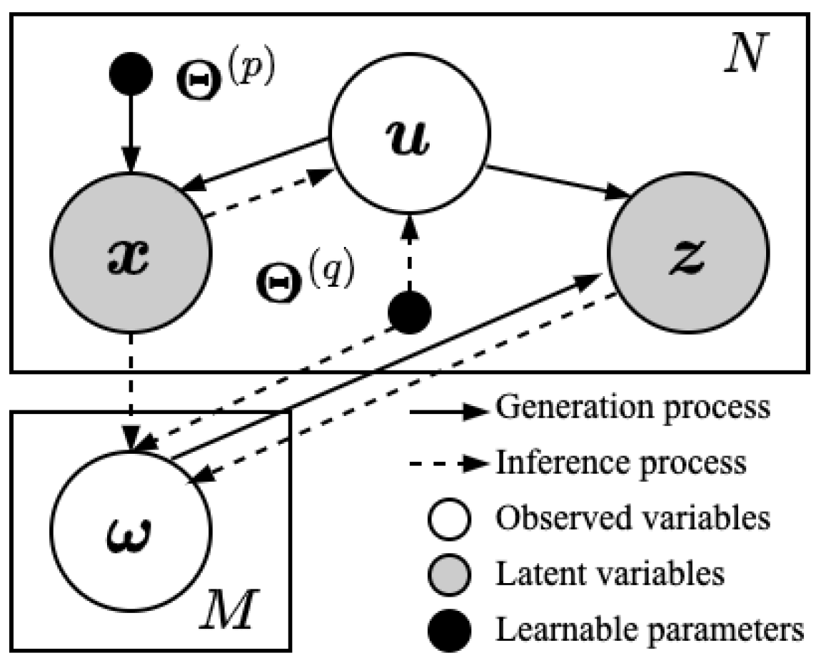
3. Methodology
- Generate a sample of the latent logits from a standard normal prior:
- Generate a sample of the confusion vector of each label from a Dirichlet prior:where the t-th element of (i.e., ) denotes the probability of the t-th label being mis-annotated as the m-th label.
- Generate a sample of the noisy label distribution from a Dirichlet distribution conditioned on the latent logits and the confusion vector:
- Generate observations of the feature variables:where is the precision of the normal distribution for generating the feature vector.
4. Variational Inference
5. Experiments
5.1. Datasets and Evaluation Metrics
5.2. Experimental Procedure
5.3. Comparison Algorithms
5.4. Results and Discussions
5.5. Further Analysis
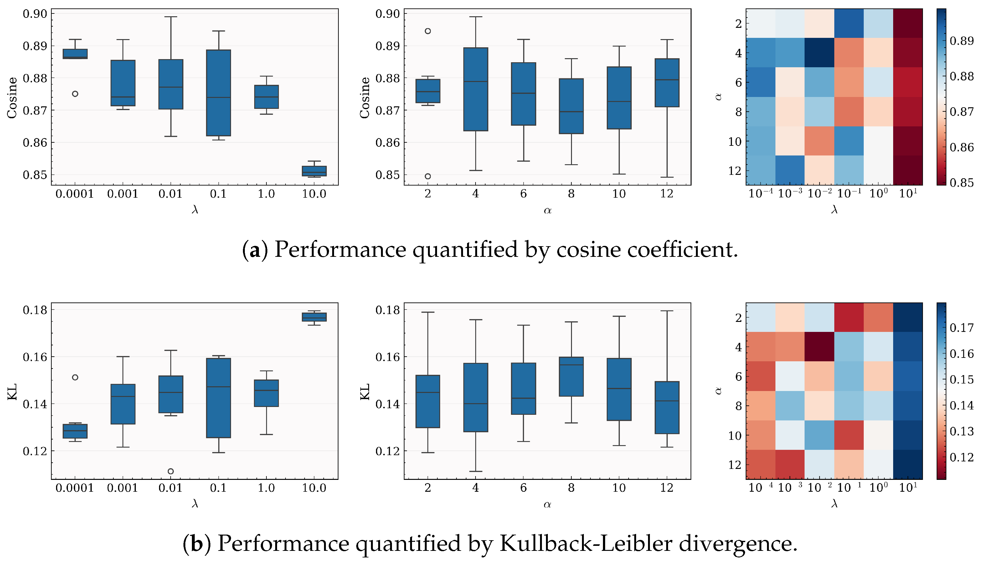
5.5.1. Hyperparameter Analysis
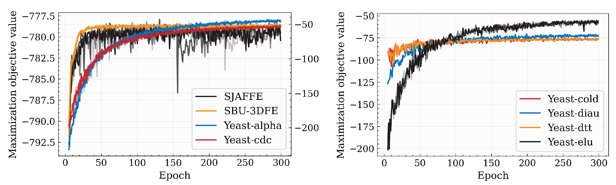
5.5.2. Convergence
6. Conclusions
Author Contributions
Funding
Data Availability Statement
Conflicts of Interest
References
- Geng, X. Label Distribution Learning. IEEE Trans. Knowl. Data Eng. 2016, 28, 1734–1748. [Google Scholar] [CrossRef]
- Geng, X.; Yin, C.; Zhou, Z.H. Facial Age Estimation by Learning from Label Distributions. IEEE Trans. Pattern Anal. Mach. Intell. 2013, 35, 2401–2412. [Google Scholar] [CrossRef] [PubMed]
- Shen, W.; Guo, Y.; Wang, Y.; Zhao, K.; Wang, B.; Yuille, A. Deep Differentiable Random Forests for Age Estimation. IEEE Trans. Pattern Anal. Mach. Intell. 2021, 43, 404–419. [Google Scholar] [CrossRef]
- Shen, W.; Zhao, K.; Guo, Y.; Yuille, A. Label Distribution Learning Forests. In Proceedings of the Advances in Neural Information Processing Systems, Long Beach, CA, USA, 4–9 December 2017. [Google Scholar]
- Hou, P.; Geng, X.; Huo, Z.W.; Lv, J. Semi-Supervised Adaptive Label Distribution Learning for Facial Age Estimation. In Proceedings of the AAAI Conference on Artificial Intelligence, San Francisco, CA, USA, 4–9 February 2017; pp. 2015–2021. [Google Scholar]
- Gao, B.B.; Zhou, H.Y.; Wu, J.; Geng, X. Age Estimation Using Expectation of Label Distribution Learning. In Proceedings of the International Joint Conference on Artificial Intelligence, Stockholm, Sweden, 13–19 July 2018; pp. 712–718. [Google Scholar]
- He, T.; Jin, X. Image Emotion Distribution Learning with Graph Convolutional Networks. In Proceedings of the International Conference on Multimedia Retrieval, Ottawa, ON, Canada, 10–13 June 2019; pp. 382–390. [Google Scholar]
- Yang, J.; Sun, M.; Sun, X. Learning Visual Sentiment Distributions via Augmented Conditional Probability Neural Network. In Proceedings of the AAAI Conference on Artificial Intelligence, San Francisco, CA, USA, 4–9 February 2017; pp. 224–230. [Google Scholar]
- Jia, X.; Zheng, X.; Li, W.; Zhang, C.; Li, Z. Facial Emotion Distribution Learning by Exploiting Low-Rank Label Correlations Locally. In Proceedings of the IEEE Conference on Computer Vision and Pattern Recognition, Long Beach, CA, USA, 16–20 June 2019; pp. 9841–9850. [Google Scholar]
- Peng, K.C.; Chen, T.; Sadovnik, A.; Gallagher, A. A Mixed Bag of Emotions: Model, Predict, and Transfer Emotion Distributions. In Proceedings of the IEEE Conference on Computer Vision and Pattern Recognition, Boston, MA, USA, 7–12 June 2015; pp. 860–868. [Google Scholar]
- Machajdik, J.; Hanbury, A. Affective Image Classification Using Features Inspired by Psychology and Art Theory. In Proceedings of the ACM International Conference on Multimedia, Florence, Italy, 25–29 October 2010; pp. 83–92. [Google Scholar]
- Ren, Y.; Geng, X. Sense Beauty by Label Distribution Learning. In Proceedings of the International Joint Conference on Artificial Intelligence, Melbourne, Australia, 19–25 August 2017; pp. 2648–2654. [Google Scholar]
- Geng, X.; Hou, P. Pre-Release Prediction of Crowd Opinion on Movies by Label Distribution Learning. In Proceedings of the International Joint Conference on Artificial Intelligence, Buenos Aires, Argentina, 25–31 July 2015; pp. 3511–3517. [Google Scholar]
- Liu, S.; Huang, E.; Zhou, Z.; Xu, Y.; Kui, X.; Lei, T.; Meng, H. Lightweight Facial Attractiveness Prediction Using Dual Label Distribution. IEEE Trans. Cogn. Dev. Syst. 2025. early access. [Google Scholar] [CrossRef]
- Tang, Y.; Ni, Z.; Zhou, J.; Zhang, D.; Lu, J.; Wu, Y.; Zhou, J. Uncertainty-Aware Score Distribution Learning for Action Quality Assessment. In Proceedings of the IEEE Conference on Computer Vision and Pattern Recognition, Seattle, WA, USA, 13–19 June 2020; pp. 9836–9845. [Google Scholar]
- Xing, C.; Geng, X.; Xue, H. Logistic Boosting Regression for Label Distribution Learning. In Proceedings of the IEEE Conference on Computer Vision and Pattern Recognition, Las Vegas, NV, USA, 27–30 June 2016; pp. 4489–4497. [Google Scholar]
- Wang, J.; Geng, X. Label Distribution Learning by Exploiting Label Distribution Manifold. IEEE Trans. Neural Netw. Learn. Syst. 2023, 34, 839–852. [Google Scholar] [CrossRef] [PubMed]
- Jia, X.; Shen, X.; Li, W.; Lu, Y.; Zhu, J. Label Distribution Learning by Maintaining Label Ranking Relation. IEEE Trans. Knowl. Data Eng. 2023, 35, 1695–1707. [Google Scholar] [CrossRef]
- Jia, X.; Qin, T.; Lu, Y.; Li, W. Adaptive Weighted Ranking-Oriented Label Distribution Learning. IEEE Trans. Neural Netw. Learn. Syst. 2024, 35, 11302–11316. [Google Scholar] [CrossRef]
- Kou, Z.; Wang, J.; Jia, Y.; Liu, B.; Geng, X. Instance-Dependent Inaccurate Label Distribution Learning. IEEE Trans. Neural Netw. Learn. Syst. 2023, 36, 1425–1437. [Google Scholar] [CrossRef]
- Guiasu, S.; Shenitzer, A. The Principle of Maximum Entropy. Math. Intell. 1985, 7, 42–48. [Google Scholar] [CrossRef]
- Zhai, Y.; Dai, J. Geometric Mean Metric Learning for Label Distribution Learning. In Proceedings of the International Conference on Neural Information Processing, Sydney, NSW, Australia, 12–15 December 2019; pp. 260–272. [Google Scholar]
- Xu, S.; Ju, H.; Shang, L.; Pedrycz, W.; Yang, X.; Li, C. Label Distribution Learning: A Local Collaborative Mechanism. Int. J. Approx. Reason. 2020, 121, 59–84. [Google Scholar] [CrossRef]
- Friedman, J.; Hastie, T.; Tibshirani, R. Additive Logistic Regression: A Statistical View of Boosting. Ann. Stat. 2000, 28, 337–407. [Google Scholar] [CrossRef]
- Zhai, Y.; Dai, J.; Shi, H. Label Distribution Learning Based on Ensemble Neural Networks. In Proceedings of the International Conference on Neural Information Processing, Siem Reap, Cambodia, 13–16 December 2018; pp. 593–602. [Google Scholar]
- Chen, M.; Wang, X.; Feng, B.; Liu, W. Structured Random Forest for Label Distribution Learning. Neurocomputing 2018, 320, 171–182. [Google Scholar] [CrossRef]
- Jia, X.; Li, W.; Liu, J.; Zhang, Y. Label Distribution Learning by Exploiting Label Correlations. In Proceedings of the AAAI Conference on Artificial Intelligence, New Orleans, LA, USA, 2–7 February 2018; pp. 3310–3317. [Google Scholar]
- Zhao, P.; Zhou, Z.H. Label Distribution Learning by Optimal Transport. In Proceedings of the AAAI Conference on Artificial Intelligence, New Orleans, LA, USA, 2–7 February 2018; pp. 4506–4513. [Google Scholar]
- Zheng, X.; Jia, X.; Li, W. Label Distribution Learning by Exploiting Sample Correlations Locally. In Proceedings of the AAAI Conference on Artificial Intelligence, New Orleans, LA, USA, 2–7 February 2018; pp. 4556–4563. [Google Scholar]
- Ren, T.; Jia, X.; Li, W.; Zhao, S. Label Distribution Learning with Label Correlations via Low-Rank Approximation. In Proceedings of the International Joint Conference on Artificial Intelligence, Macao, China, 10–16 August 2019; pp. 3325–3331. [Google Scholar]
- Ren, T.; Jia, X.; Li, W.; Chen, L.; Li, Z. Label Distribution Learning with Label-Specific Features. In Proceedings of the International Joint Conference on Artificial Intelligence, Macao, China, 10–16 August 2019; pp. 3318–3324. [Google Scholar]
- Peng, C.L.; Tao, A.; Geng, X. Label Embedding Based on Multi-Scale Locality Preservation. In Proceedings of the International Joint Conference on Artificial Intelligence, Stockholm, Sweden, 13–19 July 2018; pp. 2623–2629. [Google Scholar]
- Wang, K.; Geng, X. Binary Coding Based Label Distribution Learning. In Proceedings of the International Joint Conference on Artificial Intelligence, Stockholm, Sweden, 13–19 July 2018; pp. 2783–2789. [Google Scholar]
- Wang, K.; Geng, X. Discrete Binary Coding Based Label Distribution Learning. In Proceedings of the International Joint Conference on Artificial Intelligence, Macao, China, 10–16 August 2019; pp. 3733–3739. [Google Scholar]
- Xu, M.; Zhou, Z.H. Incomplete Label Distribution Learning. In Proceedings of the International Joint Conference on Artificial Intelligence, Melbourne, Australia, 19–25 August 2017; pp. 3175–3181. [Google Scholar]
- Zeng, X.Q.; Chen, S.F.; Xiang, R.; Wu, S.X.; Wan, Z.Y. Filling Missing Values by Local Reconstruction for Incomplete Label Distribution Learning. Int. J. Wirel. Mob. Comput. 2019, 16, 314–321. [Google Scholar] [CrossRef]
- Xu, C.; Gu, S.; Tao, H.; Hou, C. Fragmentary Label Distribution Learning via Graph Regularized Maximum Entropy Criteria. Pattern Recognit. Lett. 2021, 145, 147–156. [Google Scholar] [CrossRef]
- Xu, S.; Shang, L.; Shen, F.; Yang, X.; Pedrycz, W. Incomplete Label Distribution Learning via Label Correlation Decomposition. Inf. Fusion 2025, 113, 102600. [Google Scholar] [CrossRef]
- Jin, Y.; Gao, R.; He, Y.; Zhu, X. GLDL: Graph Label Distribution Learning. In Proceedings of the AAAI Conference on Artificial Intelligence, Vancouver, BC, Canada, 20–27 February 2024; pp. 12965–12974. [Google Scholar]
- Lu, Y.; Li, W.; Liu, D.; Li, H.; Jia, X. Adaptive-Grained Label Distribution Learning. In Proceedings of the AAAI Conference on Artificial Intelligence, Philadelphia, PA, USA, 25 February–4 March 2025; pp. 19161–19169. [Google Scholar]
- He, L.; Lu, Y.; Li, W.; Jia, X. Generative Calibration of Inaccurate Annotation for Label Distribution Learning. In Proceedings of the AAAI Conference on Artificial Intelligence, Vancouver, BC, Canada, 20–27 February 2024; pp. 12394–12401. [Google Scholar]
- Xu, N.; Tao, A.; Geng, X. Label Enhancement for Label Distribution Learning. In Proceedings of the International Joint Conference on Artificial Intelligence, Stockholm, Sweden, 13–19 July 2018; pp. 1632–1643. [Google Scholar]
- Xu, N.; Liu, Y.P.; Geng, X. Label Enhancement for Label Distribution Learning. IEEE Trans. Knowl. Data Eng. 2021, 33, 1632–1643. [Google Scholar] [CrossRef]
- Gao, Y.; Zhang, Y.; Geng, X. Label Enhancement for Label Distribution Learning via Prior Knowledge. In Proceedings of the International Joint Conference on Artificial Intelligence, Yokohama, Japan, 11–17 July 2020; pp. 3223–3229. [Google Scholar]
- Lu, Y.; Jia, X. Predicting Label Distribution from Ternary Labels. In Proceedings of the Advances in Neural Information Processing Systems, Vancouver, BC, Canada, 10–15 December 2024; pp. 70431–70452. [Google Scholar]
- Lu, Y.; Jia, X. Predicting Label Distribution from Multi-Label Ranking. In Proceedings of the Advances in Neural Information Processing Systems, New Orleans, LA, USA, 28 November–9 December 2022; pp. 36931–36943. [Google Scholar]
- Lu, Y.; Li, W.; Li, H.; Jia, X. Predicting Label Distribution from Tie-Allowed Multi-Label Ranking. IEEE Trans. Pattern Anal. Mach. Intell. 2023, 45, 15364–15379. [Google Scholar] [CrossRef] [PubMed]
- Lu, Y.; Li, W.; Li, H.; Jia, X. Ranking-Preserved Generative Label Enhancement. Mach. Learn. 2023, 112, 4693–4721. [Google Scholar] [CrossRef]
- Kingma, D.P.; Welling, M. Auto-Encoding Variational Bayes. In Proceedings of the International Conference on Learning Representations, Scottsdale, AZ, USA, 2–4 May 2013. [Google Scholar]
- Joo, W.; Lee, W.; Park, S.; Moon, I.C. Dirichlet Variational Autoencoder. Pattern Recognit. 2020, 107, 107514. [Google Scholar] [CrossRef]
- Lyons, M.; Akamatsu, S.; Kamachi, M.; Gyoba, J. Coding Facial Expressions with Gabor Wavelets. In Proceedings of the IEEE International Conference on Automatic Face and Gesture Recognition, Nara, Japan, 14–16 April 1998; pp. 200–205. [Google Scholar]
- Yin, L.; Wei, X.; Sun, Y.; Wang, J.; Rosato, M.J. A 3D Facial Expression Database For Facial Behavior Research. In Proceedings of the International Conference on Automatic Face and Gesture Recognition, Southampton, UK, 10–12 April 2006; pp. 211–216. [Google Scholar]
- Liu, X.; Zhu, J.; Zheng, Q.; Li, Z.; Liu, R.; Wang, J. Bidirectional Loss Function for Label Enhancement and Distribution Learning. Knowl.-Based Syst. 2021, 213, 106690. [Google Scholar] [CrossRef]
- Zychowski, A.; Mandziuk, J. Duo-LDL Method for Label Distribution Learning Based on Pairwise Class Dependencies. Appl. Soft Comput. 2021, 110, 107585. [Google Scholar] [CrossRef]

| Notation | Description |
|---|---|
| Inner product of vectors and | |
| D-dimensional feature space, i.e., | |
| M-dimensional distribution space, i.e., | |
| Random vector of feature variables | |
| Label distribution | |
| Multi-layer perceptron with as input and as parameters | |
| norm of a vector | |
| Composition of functions h and f, i.e., | |
| Normal distribution | |
| Dirichlet distribution |
| ID | Dataset | # Instances | # Features | # Labels |
|---|---|---|---|---|
| 1 | SJAFFE [51] | 213 | 243 | 6 |
| 2 | SBU-3DFE [52] | 2500 | 243 | 6 |
| 3 | Yeast-alpha [1] | 2465 | 24 | 18 |
| 4 | Yeast-cdc [1] | 2465 | 24 | 15 |
| 5 | Yeast-cold [1] | 2465 | 24 | 14 |
| 6 | Yeast-diau [1] | 2465 | 24 | 7 |
| 7 | Yeast-dtt [1] | 2465 | 24 | 6 |
| 8 | Yeast-elu [1] | 2465 | 24 | 6 |
| Cheb (↓) | Clark (↓) | Canber (↓) | KL (↓) | Cosine (↑) | Intersec (↑) | |
|---|---|---|---|---|---|---|
| SJAFFE | ||||||
| Ours | ||||||
| LDL-DPA | ||||||
| LDL-LDM | ||||||
| LDL-LRR | ||||||
| Duo-LDL | ||||||
| BD-LDL | ||||||
| SABFGS | ||||||
| AAkNN | ||||||
| SBU-3DFE | ||||||
| Ours | ||||||
| LDL-DPA | ||||||
| LDL-LDM | ||||||
| LDL-LRR | ||||||
| Duo-LDL | ||||||
| BD-LDL | ||||||
| SABFGS | ||||||
| AAkNN | ||||||
| Yeast-alpha | ||||||
| Ours | ||||||
| LDL-DPA | ||||||
| LDL-LDM | ||||||
| LDL-LRR | ||||||
| Duo-LDL | ||||||
| BD-LDL | ||||||
| SABFGS | ||||||
| AAkNN | ||||||
| Yeast-cdc | ||||||
| Ours | ||||||
| LDL-DPA | ||||||
| LDL-LDM | ||||||
| LDL-LRR | ||||||
| Duo-LDL | ||||||
| BD-LDL | ||||||
| SABFGS | ||||||
| AAkNN | ||||||
| Cheb (↓) | Clark (↓) | Canber (↓) | KL (↓) | Cosine (↑) | Intersec (↑) | |
|---|---|---|---|---|---|---|
| Yeast-cold | ||||||
| Ours | ||||||
| LDL-DPA | ||||||
| LDL-LDM | ||||||
| LDL-LRR | ||||||
| Duo-LDL | ||||||
| BD-LDL | ||||||
| SABFGS | ||||||
| AAkNN | ||||||
| Yeast-diau | ||||||
| Ours | ||||||
| LDL-DPA | ||||||
| LDL-LDM | ||||||
| LDL-LRR | ||||||
| Duo-LDL | ||||||
| BD-LDL | ||||||
| SABFGS | ||||||
| AAkNN | ||||||
| Yeast-dtt | ||||||
| Ours | ||||||
| LDL-DPA | ||||||
| LDL-LDM | ||||||
| LDL-LRR | ||||||
| Duo-LDL | ||||||
| BD-LDL | ||||||
| SABFGS | ||||||
| AAkNN | ||||||
| Yeast-elu | ||||||
| Ours | ||||||
| LDL-DPA | ||||||
| LDL-LDM | ||||||
| LDL-LRR | ||||||
| Duo-LDL | ||||||
| BD-LDL | ||||||
| SABFGS | ||||||
| AAkNN | ||||||
| Cheb (↓) | Clark (↓) | Canber (↓) | KL (↓) | Cosine (↑) | Intersec (↑) | |
|---|---|---|---|---|---|---|
| SJAFFE | ||||||
| Ours | ||||||
| LDL-DPA | ||||||
| LDL-LDM | ||||||
| LDL-LRR | ||||||
| Duo-LDL | ||||||
| BD-LDL | ||||||
| SABFGS | ||||||
| AAkNN | ||||||
| SBU-3DFE | ||||||
| Ours | ||||||
| LDL-DPA | ||||||
| LDL-LDM | ||||||
| LDL-LRR | ||||||
| Duo-LDL | ||||||
| BD-LDL | ||||||
| SABFGS | ||||||
| AAkNN | ||||||
| Yeast-alpha | ||||||
| Ours | ||||||
| LDL-DPA | ||||||
| LDL-LDM | ||||||
| LDL-LRR | ||||||
| Duo-LDL | ||||||
| BD-LDL | ||||||
| SABFGS | ||||||
| AAkNN | ||||||
| Yeast-cdc | ||||||
| Ours | ||||||
| LDL-DPA | ||||||
| LDL-LDM | ||||||
| LDL-LRR | ||||||
| Duo-LDL | ||||||
| BD-LDL | ||||||
| SABFGS | ||||||
| AAkNN | ||||||
| Cheb (↓) | Clark (↓) | Canber (↓) | KL (↓) | Cosine (↑) | Intersec (↑) | |
|---|---|---|---|---|---|---|
| Yeast-cold | ||||||
| Ours | ||||||
| LDL-DPA | ||||||
| LDL-LDM | ||||||
| LDL-LRR | ||||||
| Duo-LDL | ||||||
| BD-LDL | ||||||
| SABFGS | ||||||
| AAkNN | ||||||
| Yeast-diau | ||||||
| Ours | ||||||
| LDL-DPA | ||||||
| LDL-LDM | ||||||
| LDL-LRR | ||||||
| Duo-LDL | ||||||
| BD-LDL | ||||||
| SABFGS | ||||||
| AAkNN | ||||||
| Yeast-dtt | ||||||
| Ours | ||||||
| LDL-DPA | ||||||
| LDL-LDM | ||||||
| LDL-LRR | ||||||
| Duo-LDL | ||||||
| BD-LDL | ||||||
| SABFGS | ||||||
| AAkNN | ||||||
| Yeast-elu | ||||||
| Ours | ||||||
| LDL-DPA | ||||||
| LDL-LDM | ||||||
| LDL-LRR | ||||||
| Duo-LDL | ||||||
| BD-LDL | ||||||
| SABFGS | ||||||
| AAkNN | ||||||
Disclaimer/Publisher’s Note: The statements, opinions and data contained in all publications are solely those of the individual author(s) and contributor(s) and not of MDPI and/or the editor(s). MDPI and/or the editor(s) disclaim responsibility for any injury to people or property resulting from any ideas, methods, instructions or products referred to in the content. |
© 2025 by the authors. Licensee MDPI, Basel, Switzerland. This article is an open access article distributed under the terms and conditions of the Creative Commons Attribution (CC BY) license (https://creativecommons.org/licenses/by/4.0/).
Share and Cite
Li, X.; Meng, C.; Zhou, H.; Guo, Y.; Xue, B.; Yu, T.; Lu, Y. Generative Learning from Semantically Confused Label Distribution via Auto-Encoding Variational Bayes. Electronics 2025, 14, 2736. https://doi.org/10.3390/electronics14132736
Li X, Meng C, Zhou H, Guo Y, Xue B, Yu T, Lu Y. Generative Learning from Semantically Confused Label Distribution via Auto-Encoding Variational Bayes. Electronics. 2025; 14(13):2736. https://doi.org/10.3390/electronics14132736
Chicago/Turabian StyleLi, Xinhai, Chenxu Meng, Heng Zhou, Yi Guo, Bowen Xue, Tianzuo Yu, and Yunan Lu. 2025. "Generative Learning from Semantically Confused Label Distribution via Auto-Encoding Variational Bayes" Electronics 14, no. 13: 2736. https://doi.org/10.3390/electronics14132736
APA StyleLi, X., Meng, C., Zhou, H., Guo, Y., Xue, B., Yu, T., & Lu, Y. (2025). Generative Learning from Semantically Confused Label Distribution via Auto-Encoding Variational Bayes. Electronics, 14(13), 2736. https://doi.org/10.3390/electronics14132736