Model-Driven Meta-Learning-Aided Fast Beam Prediction in Millimeter-Wave Communications

Abstract

Beamforming plays a key role in improving the spectrum utilization efficiency of multi-antenna systems. However, we observe that (i) conventional beam prediction solutions suffer from high model training overhead and computational latency and thus cannot adapt quickly to changing wireless environments, and (ii) deep-learning-based beamforming may face the risk of catastrophic oblivion in dynamically changing environments, which can significantly degrade system performance. Inspired by the above challenges, we propose a continuous-learning-inspired beam prediction model for fast beamforming adaptation in dynamic downlink millimeter-wave (mmWave) communications. More specifically, we develop a meta-empirical replay (MER)-based beam prediction model. It combines empirical replay and optimization-based meta-learning. This approach optimizes the trade-offs between transmission and interference in dynamic environments, enabling effective fast beamforming adaptation. Finally, the high-performance gains brought by the proposed model in dynamic communication environments are verified through simulations. The simulation results show that our proposed model not only maintains a high-performance memory for old tasks but also adapts quickly to new tasks.

1. Introduction

Massive multiple-input multiple-output (MIMO) communication stands out as an indispensable technology for the advancement of the sixth-generation (6G) mobile communication system [1,2,3,4,5,6]. This innovative approach, which leverages an extensive array of antennas, not only significantly amplifies the system’s capacity but also boosts data transmission rates. Metasurfaces [7], which can be integrated with MIMO systems to further enhance their performance by shaping the propagation environment and improving signal quality, are also gaining attention in this context. Consequently, they play a crucial role in addressing the ever-increasing demand for swift and efficient wireless communication capabilities in the forthcoming era of next-generation millimeter-wave (mmWave) systems. The strategic importance of MIMO in this context is further underscored by recent research findings as cited in references [8,9], highlighting its potential to revolutionize the landscape of wireless connectivity.

However, mmWave MIMO systems face significant challenges, including severe path loss and high user interference, which can limit coverage and degrade performance. These challenges are exacerbated by the high frequency of mmWave signals, which are highly susceptible to attenuation over distance, further complicating the deployment of reliable and efficient communication systems.

Beamforming is a crucial solution to these challenges, as it can compensate for path loss and reduce multi-user interference [10]. By steering the transmission beams towards desired users and away from interfering ones, beamforming improves the signal-to-noise ratio (SNR) and enhances overall system performance. However, current beamforming optimization methods often rely on iterative solutions that suffer from slow convergence and computational delays, making them unsuitable for real-time 5G systems. Therefore, developing beamforming solutions that reduce computational burden while maintaining performance has become a critical concern. Researchers are actively exploring innovative approaches, such as leveraging machine learning and artificial intelligence techniques, to develop more efficient and adaptive beamforming algorithms. These efforts aim to strike a balance between computational complexity and performance, thereby paving the way for the successful integration of mmWave MIMO systems into future wireless networks.

In this context, the development of advanced beamforming techniques is essential for overcoming the limitations of current methods. Traditional beamforming algorithms, which often require extensive computational resources and time-consuming optimization processes, are not well-suited for the dynamic and high-frequency nature of mmWave MIMO systems. As a result, there is a growing need for new approaches that can provide real-time adaptation and optimization of beamforming parameters. Machine learning and artificial intelligence techniques offer a promising solution to this problem, as they can enable the development of adaptive beamforming algorithms that can quickly respond to changes in the communication environment. By leveraging the power of these advanced techniques, researchers aim to develop beamforming solutions that are both efficient and effective, capable of meeting the stringent requirements of next-generation wireless communication systems.

In summary, massive MIMO is a critical technology for the advancement of 6G communication systems, offering significant improvements in system capacity and data transmission rates. However, mmWave MIMO systems face challenges such as severe path loss and high user interference, which can limit their performance. Beamforming is a key solution to these challenges, but current methods suffer from slow convergence and computational delays. By leveraging machine learning and artificial intelligence techniques, researchers are developing more efficient and adaptive beamforming algorithms that balance computational complexity and performance. These efforts are essential for the successful integration of mmWave MIMO systems into future wireless networks.

1.1. Relevant Research

In the rapidly evolving landscape of wireless communication, the quest for efficient and robust system design has become increasingly challenging due to the complex and dynamic nature of wireless propagation environments. Traditional methods, while effective in simpler scenarios, often fall short when confronted with the computational burden and complexity associated with modeling these highly nonlinear processes, resulting in suboptimal performance. Against this backdrop, deep learning (DL) has emerged as a game-changing technology, offering a powerful alternative that can model complex nonlinear processes at low complexity [11,12]. This capability is particularly crucial in wireless communication systems, where the propagation environment is highly dynamic and nonlinear. DL leverages the power of neural networks to approximate these complex relationships efficiently. By training on large datasets, DL models can learn to capture the intricate patterns in wireless channels, enabling more accurate predictions and optimizations with significantly reduced computational overhead. This makes DL an attractive solution for addressing the challenges in modern wireless communication systems, where low-latency and high-throughput operations are essential.

In the field of wireless communications, DL has had a wide range of applications in terms of channel estimation and decoding [13,14], hybrid beamforming techniques [15,16], and optimal resource allocation [17,18]. For channel estimation, DL-based methods have shown remarkable improvements in accuracy and robustness compared to conventional techniques. These methods leverage the ability of DL models to learn from large datasets and adapt to varying channel conditions, thereby enhancing the reliability and performance of wireless communication systems. In the context of hybrid beamforming [19,20], DL has been used to optimize beamforming weights and improve signal quality in complex environments. This is particularly important in modern wireless systems, where beamforming plays a vital role in managing interference and maximizing spectral efficiency. Additionally, DL has been applied to optimal resource allocation, where it helps in dynamically adjusting power levels, frequency bands, and other resources to meet the varying demands of users. These applications demonstrate the versatility and effectiveness of DL in addressing diverse challenges in wireless communications.

The effectiveness of DL techniques in the area of resource allocation [17,18] is largely due to its optimization framework, which utilizes deep neural networks (DNNs) to learn direct mappings between inputs and outputs rather than directly solving complex mathematical optimization problems [21,22,23]. Traditional optimization methods often require solving complex mathematical problems, which can be computationally intensive and time-consuming. In contrast, DL-based approaches bypass this complexity by training neural networks to directly map system inputs to optimal resource allocation strategies. This not only reduces the computational burden but also allows for faster adaptation to dynamic changes in the communication environment. For example, recent studies have demonstrated that DL can effectively optimize power control and resource allocation in real-time, significantly improving system throughput and user satisfaction. By learning from historical data and continuously adapting to new scenarios, DL models can provide near-optimal solutions with minimal computational effort, making them highly attractive for practical deployment in next-generation wireless networks.

In the field of wireless communications, beamforming is a key technology that can significantly improve the quality and efficiency of signal transmission. However, traditional direct prediction methods often require neural networks to deal with complex input/output mapping relationships when implementing beamforming, which not only increases the complexity of the model but also raises the difficulty of training. This high-complexity training process may lead to excessive training time and even become infeasible in resource-constrained environments. To address this challenge, the literature [24] proposes beamforming neural networks (BNNs) based on the optimal solution structure, which effectively reduces the complexity of prediction by predicting intermediate variables instead of directly predicting the final result. Reference [25] focuses on designing a dual-ascent-inspired transmit precoding approach for massive MIMO systems so as to provide a global optimum solution to the challenging non-convex quadratically constrained quadratic program (QCQP) problem with low complexity.

The core advantage of this method is that it utilizes the optimal solution structure in the beamforming problem to guide the learning process of the neural network. By constructing a structured model that captures the key features and constraints of the beamforming problem, the BNNs are able to learn the intrinsic laws of the problem more efficiently. This structured learning approach not only reduces the number of parameters that the network needs to learn and reduces the amount of computation but also improves the generalization ability of the model and the learning efficiency. In addition, since the model is designed based on the structure of the optimal solution, it provides a more flexible and interpretable solution, which is very useful for practical system design and optimization. Also, this model is easier to integrate with other system components as it provides a more standardized and modular interface. Thus, BNNs based on optimal solution structures provide an efficient, flexible, and interpretable new approach to beamforming problems in wireless communications.

Today, channel dynamics are a key issue in wireless communications, especially in mmWave and MIMO systems. These systems face significant path loss and high user interference, limiting coverage and degrading performance [6]. The dynamic change of the channel not only affects the transmission quality of the signal but also poses a challenge to the resource allocation and beamforming strategy of the system [13,14,15]. Therefore, understanding and modeling the dynamics of channels is critical to improving system performance.

To grasp the dynamic nature of the channel, it is crucial to examine the contributing factors. These include user mobility, environmental changes, and signal propagation characteristics. User mobility alters the channel’s statistical properties as the distance between the transmitter and receiver changes, causing variations in path loss and multipath fading. Environmental variations, such as changes in buildings, vegetation, and weather, also affect the channel. Additionally, signal propagation characteristics like reflection, refraction, and scattering add to the channel’s complexity. Together, these factors create a highly dynamic and complex channel environment, posing significant challenges for designing efficient communication systems.

However, the works mentioned above assume that training and testing environments have the same distribution. If this assumption fails, the trained model’s performance will significantly deteriorate in new environments, a phenomenon known as catastrophic forgetting [26]. This has become a major challenge for DL in wireless communication, along with the dynamics of the scenarios in [27,28,29,30].

Continuous learning (CL), as an advanced machine learning method, is gradually gaining wide attention from researchers in the field of wireless communications. This method is particularly suitable for those scenarios that require constant adaptation to new environments and tasks. In this area, notable contributions have been made to the literature [31,32] that focus on dynamic resource optimization using data-driven methods such as deep learning. Specifically, the literature [31] proposes a model-driven CL framework dedicated to dynamic beamforming, a framework that continuously optimizes beamforming strategies through continuous learning to adapt to changing communication environments. In addition the literature [32] further develops this approach by developing a two-tier optimization method for wireless resource allocation, which improves the efficiency and flexibility of resource allocation by optimizing at different levels. Although these approaches are theoretically innovative, in practice they require storing a large amount of data on the mobile station, which not only limits the flexibility of the system but also significantly increases the storage overhead.

1.2. Contribution

In this paper, we propose a communication scenario model that is closer to real-world applications and takes into account dynamically changing channel conditions [33], as shown in Figure 1; although the channel distribution remains consistent over a single time period, the statistical properties of the channel change over time. This variation poses a challenge to well-trained DL models, as their performance tends to degrade significantly once they are deployed in new dynamic environments. In such dynamic environments, where data is generated sequentially and the dataset collected at each time slot is labeled $D_t$, a training strategy that is based only on the data $D_t$ of the current time slot and ignores the data of previous time slots can lead to the severe catastrophic forgetting problem. This phenomenon can lead to a drastic performance degradation of the model when facing new environments, thus limiting the potential application of DL [26] in real communication systems.

In addition, our meta-experience replay (MER)-based beam prediction method is able to achieve high sum-rate performance while maintaining low complexity. This approach is not only theoretically innovative but also has high application value in practical systems as it can effectively balance performance and resource consumption, providing a new solution for the wireless communication field. The main contributions of this paper are summarized as follows:

• Firstly, we use experience replay to select key data for storage, supporting effective learning while retaining old tasks. Then, we optimize neural network parameters $\theta$ to balance new task adaptation and old task retention.
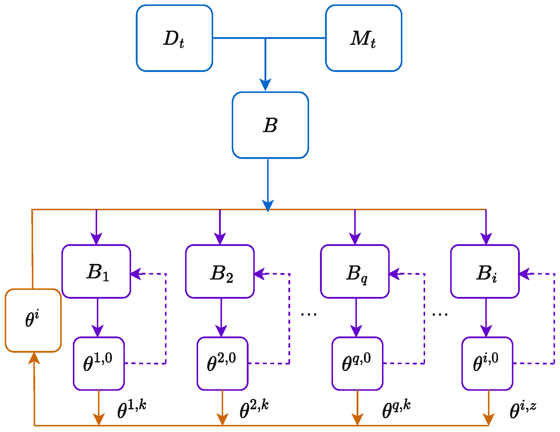
• In addition, we propose an optimization strategy for beam prediction based on MER. The data samples selected through the experience playback strategy are fed back to the main hierarchy to influence the update of the weights $\theta$. This model is able to learn a new task while maintaining the memory of the old task, realizing the goal of continuous learning.
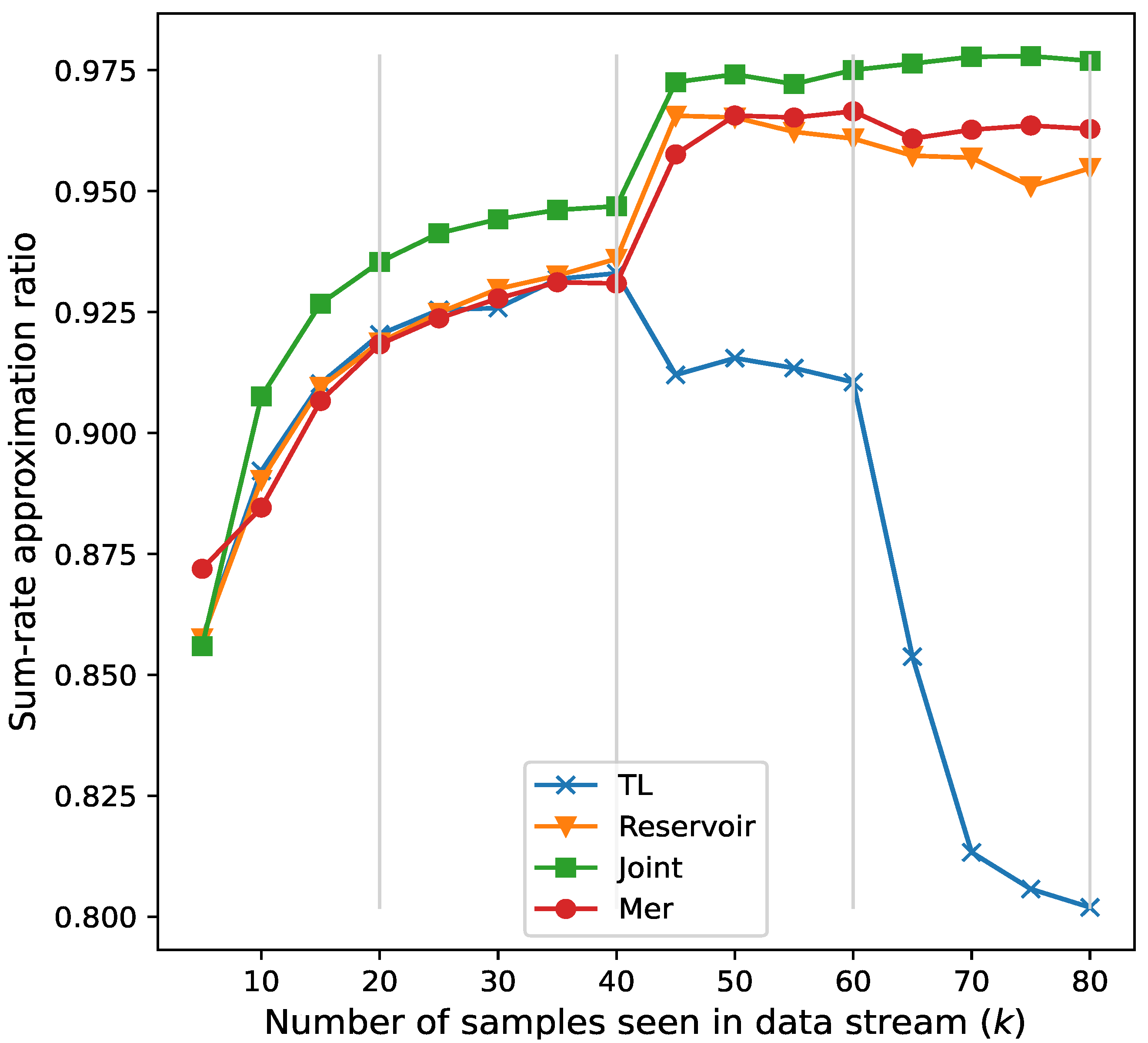
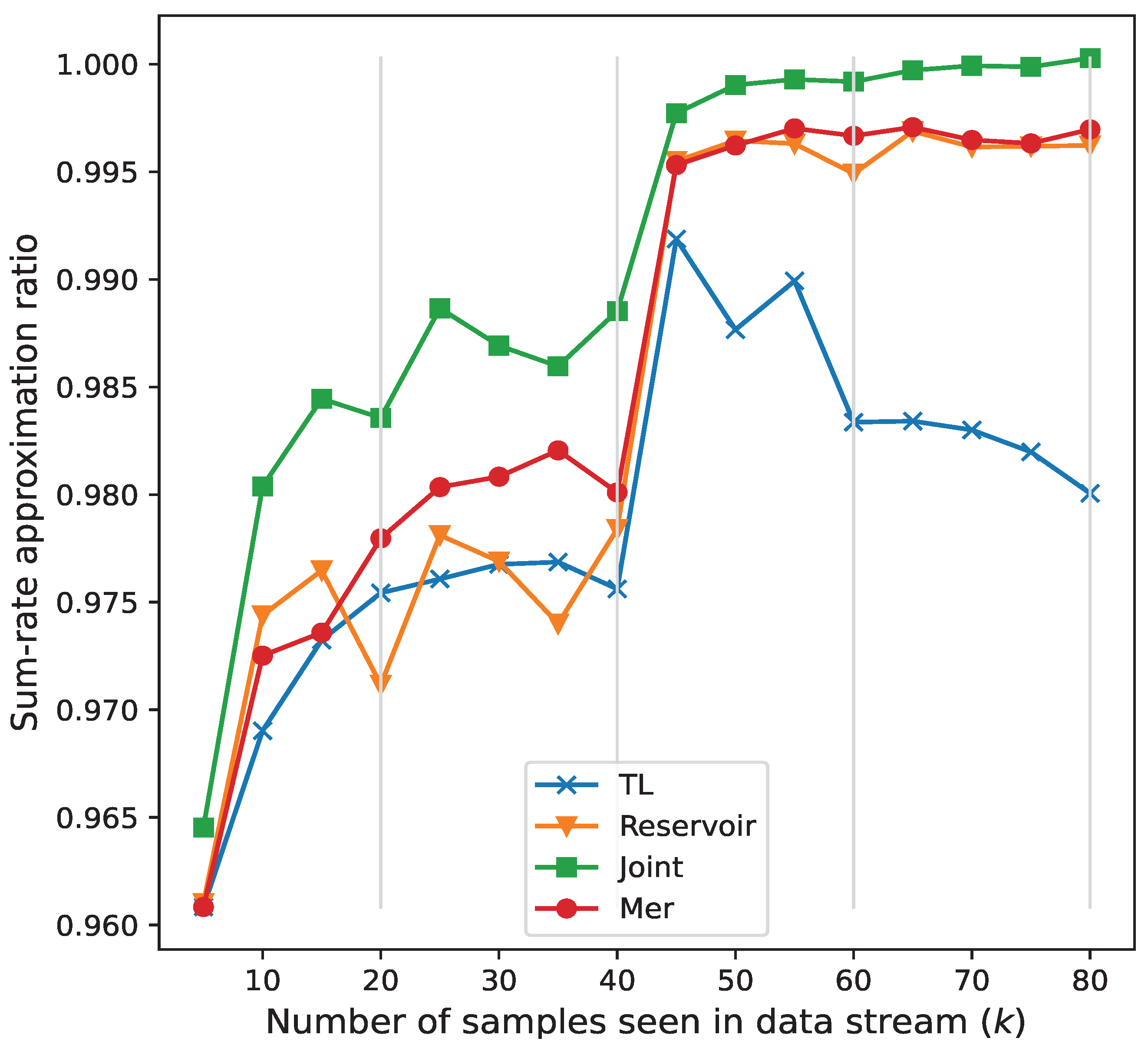
• Finally, we propose an MER-based continuous learning beam prediction model for dynamic downlink multiple-input single-output (MISO) systems. The model uses meta-learning to optimize beamforming and adapt quickly to dynamic environments. Experiments show that it outperforms transfer learning (TL) [26] and Reservoir [34], maintaining strong performance in dynamic task assignments.

• Notations: The boldface lowercase letters and capital letters are used to represent column vectors and matrices, respectively. ${|·|}^2$ is the square of the modulus used to compute the vector, and the notation $Tr(·)$ represents the trace operator of the matrix. The notation $a^H$ denotes the Hermitian conjugate transpose of a vector, and $\mathcal{CN}(M,K)$ denotes the Gaussian distribution.

2. System Model and Problem Formulation

Consider a downlink MISO broadcast channel system in which a base station (BS) is assumed to be equipped with N antennas to serve K single-antenna users (UEs). Then, the signal observed at the kth UE can be expressed as

$$\begin{array}{c}\hfill y_k={\mathbf{h}}_k^H{\mathbf{v}}_k{s}_k+\sum _{i=1,i\ne k}^K{\mathbf{h}}_k^H{\mathbf{v}}_i{s}_i+n_k,\end{array}$$

(1)

where ${\mathbf{v}}_i\in {\mathbb{C}}^M$ is the transmit beamforming vector for user i. Let $s_i\sim$$\mathcal{CN}(0,1)$ be the independent data symbol transmitted to the ith user, and ${\mathbf{h}}_i\sim \mathcal{CN}(\mathbf{0},{\mathbf{I}}_M)$ denotes the channel between the BS and the ith UE.

The signal-to-interference-plus-noise ratio (SINR) is given by

$${\mathbf{SINR}}_k={\displaystyle \frac{|{\mathbf{h}}_k^H{\mathbf{v}}_k{|}^2}{{\sum }_{i=1,i\ne k}^K{|{\mathbf{h}}_k^H{\mathbf{v}}_i|}^2+{\sigma }^2}},$$

(2)

constrained by the transmit power; assuming that its maximum transmission power is P and α_k is the user weight of the kth user, then the weighted sum rate (WSR) maximization problem of the downlink channel with respect to the total transmit power constraint can be expressed based on the channel knowledge as

$$\begin{array}{c}\underset{\mathbf{V}}{max}\sum _{k=1}^K{\alpha }_k{\log }_2(1+{\mathbf{SINR}}_k)\hfill \\ s.t.Tr\left({\mathbf{VV}}^H\right)\le P,\hfill \end{array}$$

(3)

where $Tr(·)$ denotes the trace of a square matrix operation. $\mathbf{V}$ = $[{\mathbf{v}}_1,\dots ,{\mathbf{v}}_K]$ ∈ ${\mathbb{C}}^{N\times K}$ is the transmit beamforming matrix for K UEs at each time instance.

3. MER-Based Beam Prediction Optimization

In this section, we detail an innovative optimization strategy based on meta-learning and experience replay, specifically for dynamic beamforming in mmWave communication systems. The core of this strategy lies in the meta-learning technique, which enables the system to quickly adapt to new tasks and environments and at the same time effectively retains and utilizes the previously accumulated knowledge and experience by means of the experience replay mechanism. Through this organic combination, the strategy not only achieves efficient real-time learning but also significantly improves the optimization performance of beamforming. Details are as follows.

3.1. Beamforming Vector Decomposition

As the number of transmitting antennas and users increases, directly estimating the beamforming matrix imposes a heavy training burden on neural networks. To address this, we decompose the beamforming vector prediction into three lower-dimensional components, inspired by [35,36]. These components are then recombined via Equation (4) to form the beamforming vector for each user. This approach effectively reduces the prediction complexity by decomposing and reorganizing the process. Thus, the beamforming vector for the kth user can be formulated as

$${\mathbf{v}}_k={\alpha }_k{u}_k{w}_k{\mathbf{h}}_k{(\mathbf{S}+\mu \mathbf{I})}^{-1},$$

(4)

where $\mathbf{S}\triangleq {\sum }_{k=1}^K{\alpha }_k{\left|u_k\right|}^2{w}_k{\mathbf{h}}_k{\mathbf{h}}_k^H$, and $\mu$ ≥ 0 is a Lagrange multiplier.

In summary, the weighted minimum mean square error (WMMSE) algorithm first initializes V so that it satisfies the power constraints. Subsequently, it is iteratively updated according to the above equation until the stopping criterion is satisfied, where ${\alpha }_k$ is the system weight of user k, which is a value controlled by the communication system. The expressions $w_k$ and ${\mu }_k$ are as follows for the beamforming vector of the receiving user k and the positive user weight of user k, respectively, while $\mu$ is a Lagrange multiplier attached to the power constraints when finding the first-order optimality condition of the beamforming matrix in the WMMSE.

$$w_k={\displaystyle \frac{{{\sum }_{j=1}^K\left|{\mathbf{h}}_k^H{\mathbf{v}}_j\right|}^2+{\sigma }^2}{{\sum }_{j=1,j\ne k}^K{\left|{\mathbf{h}}_k^H{\mathbf{v}}_j\right|}^2+{\sigma }^2}},$$

(5)

$$u_k={\displaystyle \frac{{\mathbf{h}}_k^H{\mathbf{v}}_k}{{\sum }_{j=1}^K{\left|{\mathbf{h}}_k^H{\mathbf{v}}_j\right|}^2+{\sigma }^2}}.$$

(6)

In the training phase, we employ three independent neural networks, each responsible for predicting the three basic components of the beamforming vector: U, W, and $\mu$. The training starts with a random initial value of V, followed by the prediction of U and W using the current estimate of V, while $\mu$ is determined by a dichotomous search method, which is different from the neural network prediction approach employed in our method. This iterative process is similar to the WMMSE algorithm, which continues until a preset error criterion is reached. The difference is that the method in this paper simplifies the iterative process by directly predicting U, W, and $\mu$ through neural networks and reconstructing the value of V based on these predictions.

In the training phase, we specifically design the loss function by referring to [35], which is defined as the negative value of the WSR as follows:

$$R\left(i\right)=\log det(\mathbf{I}+{\mathbf{h}}_i{\mathbf{v}}_i{\mathbf{v}}_i^H{\mathbf{h}}_i^H{(\sum _{j\ne i}^K{\mathbf{h}}_j{\mathbf{v}}_j{\mathbf{v}}_j^H{\mathbf{h}}_j^H+{\sigma }^2\mathbf{I})}^{-1}),$$

(7)

$$L\left(v\right)=-\sum _{i=1}^{K}R\left(i\right).$$

(8)

3.2. A System for Learning to Learn Without Forgetting

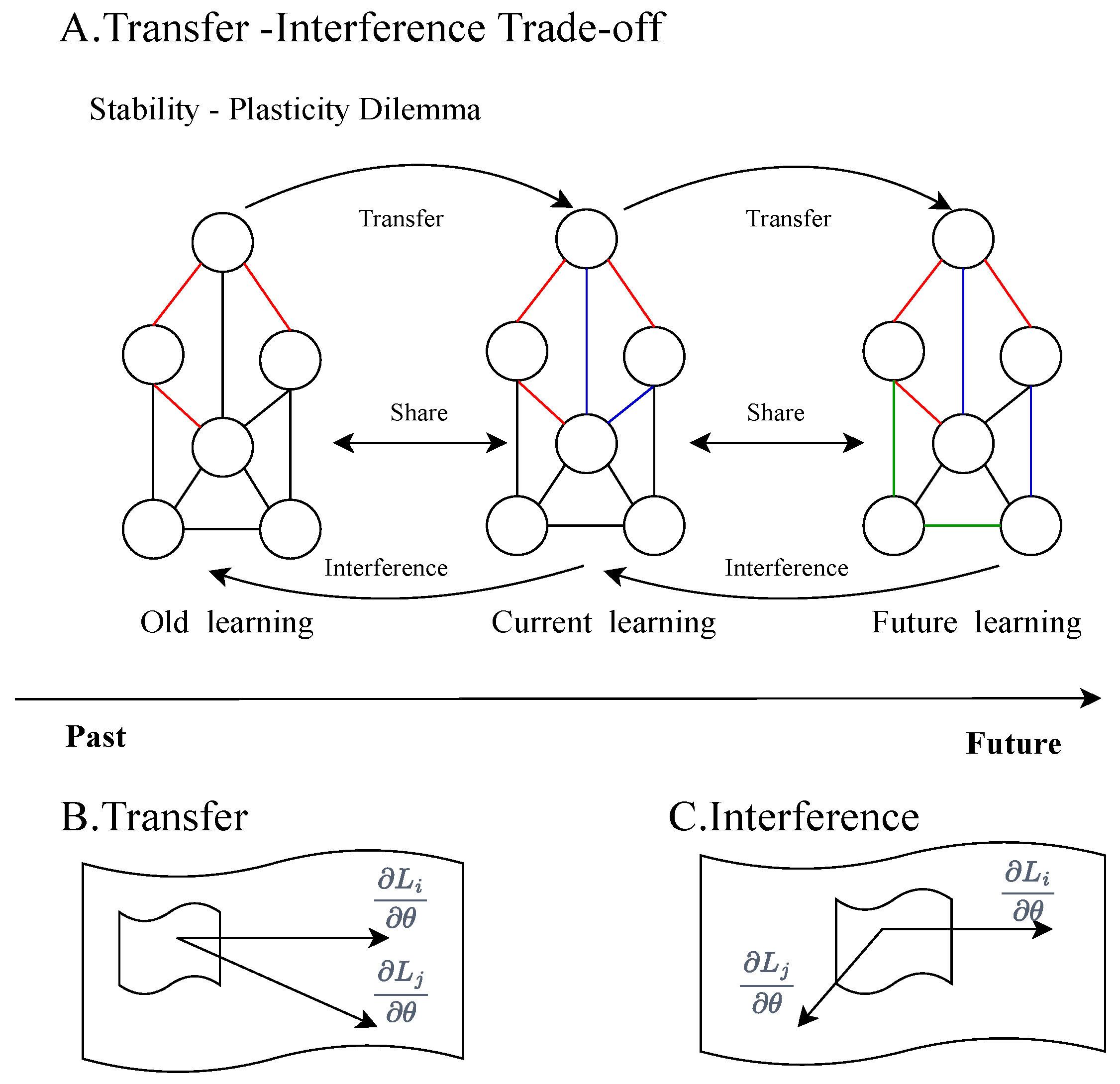
Neural network models need to allow the model to acquire new knowledge in real time and combine it with the current model as insight classes or tasks emerge. If only the current set of examples is considered in an ever-changing environment, performance on older data may suddenly degrade, a phenomenon known as catastrophic forgetting. This behavior is also infeasible if all examples are stored, requiring training from scratch. CL methods aim to train neural network samples from non-i.i.d. data streams, thus mitigating catastrophic forgetting while limiting computational cost and memory footprint.

Figure 2 in this paper demonstrates the concepts of the stability–plasticity dilemma and the transfer–interference trade-off [37,38].

(A)

The trade-off between stability and malleability is a long-standing challenge in the field of machine learning, especially in continuous or lifelong learning scenarios. This dilemma concerns how to effectively maintain stability with respect to old knowledge while learning the current task. If a learning system is too stable, it may exhibit low plasticity when integrating new knowledge, making it difficult to adapt to new tasks or environmental changes. Conversely, if a system is too malleable, it may quickly forget old tasks as it learns new ones, a phenomenon known as catastrophic forgetting [39,40,41]. To address this problem, researchers have been exploring how to find the right balance between stability and plasticity so that the learning system can learn new knowledge while maintaining mastery of old knowledge. This balance is crucial for improving the overall performance and adaptability of learning systems, especially in application scenarios that require long-term memory and rapid adaptation to new situations.

(B)

A portion of what is shown in the figure reveals the phenomenon of shifting in the weight space, a phenomenon that indicates the potential positive impact that may be exerted on older tasks when learning the current task. In machine learning models, if the gradient directions of different tasks are the same or very close to each other, learning one of them may not only improve the performance of that task but may also positively contribute to the performance of other tasks. This phenomenon is particularly important in multi-task learning or continuous learning environments because it implies that the efficiency and effectiveness of the model in dealing with diverse tasks can be improved by effectively sharing and transferring knowledge. The consistency of this gradient can be viewed as the existence of some form of knowledge association between different tasks, allowing the model to reuse existing knowledge when learning a new task, leading to faster adaptation and better generalization capabilities.

(C)

The other part describes the interference phenomenon in the weight space, which is the opposite of transfer and refers to the negative impact on the old task when learning the current task. When the gradients of the old and new tasks are in opposite or conflicting directions, learning the new task may result in forgetting the knowledge of the old task or performance degradation. All in all, this figure aims to illustrate how to maintain the memory of the old task while learning the new task in a CL environment and how to balance the learning of the old and new tasks by sharing the weights in a reasonable way to avoid catastrophic forgetting. The algorithm proposed in the paper is designed to address this problem by optimizing this trade-off through experience playback and meta-learning.

In this paper, in order to effectively deal with the catastrophic forgetting problem that may occur during the training process of dynamic scenarios, we propose an innovative continuous learning beam prediction model based on MER [42].

The MER method is a state-of-the-art machine learning strategy that skillfully combines empirical replay and optimization-based meta-learning techniques. The core goal of this approach is to enhance the performance and adaptability of neural networks in the face of non-stationary data distributions by maximizing the knowledge transfer from one task to another and minimizing the disturbances that may occur during the continuous learning process.

The MER model intelligently leverages knowledge from previous tasks to facilitate learning new tasks, reducing the forgetting of old knowledge. This strategy enhances the model’s adaptation speed to new environments and maintains performance in dynamic task assignments, which is crucial for beamforming optimization in wireless communication systems.

3.3. Experience Reply Based CL

The memory-based application dynamically adapts to scene transitions by capturing a representative subset of $M_t$ from historical training data. Specifically, key samples from the past scene data $D_{0:t-1}$ are selected to populate a fixed-size memory $M_t$ and the neural network is trained at each time step t using $M_t$ ∪ $D_t$.

Experience replay [43] is widely used in dynamic deep learning scenarios and aims to maintain memory of encountered scenarios by integrating them with current training data, stabilizing the training process. This concept can be mathematically expressed in Equation (9),

$$\begin{array}{c}\hfill \theta =arg\underset{\theta }{min}{\mathbb{E}}_M\left[L\left(v\right)\right],\end{array}$$

(9)

where M has a current size $M_{size}$ and maximum size $M_{max}$. Reservoir sampling is a random technique that maintains a fixed-size buffer to draw representative samples from a continuous data stream. When the buffer is not full, new samples are added directly. If full, samples are replaced with equal probability. This ensures each sample’s inclusion probability is the ratio of buffer size to the total observed samples.

In this paper, we use reservoir sampling to maintain an experience replay buffer with capacity $M_{size}$ and maximum capacity $M_{max}$. This method ensures that all previously encountered samples $D_{t-1}$ are stored in the buffer with equal probability, specifically $M_{size}/D_{t-1}$. The specific Algorithm 1 for Reservoir Sampling to perform empirical playback is as follows, where s is the size of the $D_t$.

In a continuous learning environment, the algorithm dynamically processes a non-static data stream, prioritizing the most recent sample for its up-to-date information. It optimizes this sample using random samples from the buffer in each iteration, ensuring equal training probability for each sample. This balances responsiveness to new data and retention of old data.

Algorithm 1 Proposed MER-Based Beam Prediction Strategy

1: Input: Initial the parameter model $\theta$ and the memory buffer M, which has a maximum capacity of $M_{max}$, beamforming matrix V, counter of time slots $t=0$.   2: We decompose the beamforming matrix into low-dimensional vectors w, u and $\mu$ and predict the three status vectors.   3: for  $T=1,2\dots$do   4:     if $M_{T-1}\cup D_T$ <$M_{max}$ then $$M_t=M_{T-1}\cup D_T$$   5:     else   6:           for $l=1,\dots ,s$ do      \\F denotes an equation representing the selection of a random number. $$j=F(min=0,max=N)$$ $$M_t=M_{T-1}\cup D_T^l$$   7:           end for   8:     end if   9: end for 10: for  $t=1,\dots ,T$  do 11: Predict the instantaneous values of the low-dimensional components $u_t$, $w_t$, ${\mu }_t$ and reconstruct the beamforming matrix according to (4). 12: According to the minimization loss function in (7) and (8), batches of size k are randomly selected from memory for in-batch updating. 13: end for 14: for  $t=1,\dots ,T$  do 15: Predict the instantaneous values of the low-dimensional components $u_t$, $w_t$, ${\mu }_t$ and reconstruct the beamforming matrix according to (4). 16: Perform cross-batch updates. 17: end for

3.4. Meta-Learning Based Experience Replay Optimization

First-Order MAML (FOMAML) [44] and Reptile [45] are both efficient meta-learning algorithms designed to quickly adapt to new tasks by omitting the calculation of the second-order derivatives and using only the first-order derivatives. FOMAML reduces complexity by simplifying the computational process of MAML while maintaining performance comparable to that of the full MAML, suggesting that model improvement relies heavily on gradient information. Reptile further simplifies the computation process by performing gradient updates on multiple tasks to adjust the model parameters, making it possible to quickly fine-tune the model to new tasks.The optimization objective of Reptile for a set of s batches can be approximated as

$$\begin{array}{c}\hfill \begin{array}{cc}\hfill {\theta }_u=& arg\underset{{\theta }_u}{min}{\mathbb{E}}_{\mathbb{D}}[2\sum _{i=1}^s[L\left(V_{B_i}\right)-\sum _{j=1}^{i-1}\alpha {\displaystyle \frac{\partial L\left(V_{B_i}\right)}{\partial {\theta }_u}}·{\displaystyle \frac{\partial L\left(V_{B_j}\right)}{\partial {\theta }_u}}]],\hfill \end{array}\end{array}$$

(10)

$$\begin{array}{c}\hfill \begin{array}{cc}\hfill {\theta }_w=& arg\underset{{\theta }_w}{min}{\mathbb{E}}_{\mathbb{D}}[2\sum _{i=1}^s[L\left(V_{B_i}\right)-\sum _{j=1}^{i-1}\alpha {\displaystyle \frac{\partial L\left(V_{B_i}\right)}{\partial {\theta }_w}}·{\displaystyle \frac{\partial L\left(V_{B_j}\right)}{\partial {\theta }_w}}]],\hfill \end{array}\end{array}$$

(11)

$$\begin{array}{c}\hfill \begin{array}{cc}\hfill {\theta }_{\mu }=& arg\underset{{\theta }_{\mu }}{min}{\mathbb{E}}_{\mathbb{D}}[2\sum _{i=1}^s[L\left(V_{B_i}\right)-\sum _{j=1}^{i-1}\alpha {\displaystyle \frac{\partial L\left(V_{B_i}\right)}{\partial {\theta }_{\mu }}}·{\displaystyle \frac{\partial L\left(V_{B_j}\right)}{\partial {\theta }_{\mu }}}]],\hfill \end{array}\end{array}$$

(12)

where $B_1,\dots ,B_s$ are batches within D. In addition, $\alpha$ denotes the learning rate, which is used to control the step size of gradient descent for each sample. In this paper, we integrate the Reptile algorithm with experience replay to enhance continuous learning, aiming to maximize migration and minimize interference. Since the Reptile objective is only partially achievable in online learning, we propose that the MER algorithm needs to optimize the following objectives in continuous learning:

$$\begin{array}{c}\hfill {\theta }_u=arg\underset{{\theta }_u}{min}{\mathbb{E}}_{\mathbb{M}}[2\sum _{i=1}^s\sum _{j=1}^k[L\left(v_{i,j}\right)-\sum _{q=1}^{i-1}\sum _{r=1}^{j-1}\alpha {\displaystyle \frac{\partial L\left(v_{i,j}\right)}{\partial {\theta }_u}}·{\displaystyle \frac{\partial L\left(v_{q,r}\right)}{\partial {\theta }_u}}]],\end{array}$$

(13)

$$\begin{array}{c}\hfill {\theta }_w=arg\underset{{\theta }_w}{min}{\mathbb{E}}_{\mathbb{M}}[2\sum _{i=1}^s\sum _{j=1}^k[L\left(v_{i,j}\right)-\sum _{q=1}^{i-1}\sum _{r=1}^{j-1}\alpha {\displaystyle \frac{\partial L\left(v_{i,j}\right)}{\partial {\theta }_w}}·{\displaystyle \frac{\partial L\left(v_{q,r}\right)}{\partial {\theta }_w}}]],\end{array}$$

(14)

$$\begin{array}{c}\hfill {\theta }_{\mu }=arg\underset{{\theta }_{\mu }}{min}{\mathbb{E}}_{\mathbb{M}}[2\sum _{i=1}^s\sum _{j=1}^k[L\left(v_{i,j}\right)-\sum _{q=1}^{i-1}\sum _{r=1}^{j-1}\alpha {\displaystyle \frac{\partial L\left(v_{i,j}\right)}{\partial {\theta }_{\mu }}}·{\displaystyle \frac{\partial L\left(v_{q,r}\right)}{\partial {\theta }_{\mu }}}]].\end{array}$$

(15)

In our beam prediction model, the MER algorithm plays a pivotal role. Its core objective is two-pronged: first, to mitigate interference between various tasks, and second, to expedite knowledge migration. Through the meticulous optimization of gradient alignment, we aim to ensure that when model parameters are shared across different tasks, the gradient direction of each task remains as consistent as feasible.

In the context of multi-task learning and continuous learning, models need to continuously adapt to new tasks while making full use of the knowledge and experience accumulated in past tasks. This consistency is a core element in achieving positive knowledge transfer. By maintaining consistency, the model is able to seamlessly integrate and utilize the knowledge accumulated in previous tasks as it learns new tasks. This seamlessness not only avoids conflicts between old and new knowledge but also provides the model with a solid knowledge base that enables it to cope with new challenges more efficiently. This gradient-aligned optimization strategy ensures that the learning goals between different tasks do not hinder each other by subtly adjusting the direction of parameter updates during the learning process.

Instead, this strategy promotes synergy between tasks. It allows the past learning outcomes to not only be preserved but also further enhance the model’s performance in new tasks. This optimization strategy enables the model to rapidly adjust parameters and adapt to new environments, mitigating performance degradation during task switching. By balancing learning efficiency and multi-task performance, it reduces training time for new tasks while maintaining high accuracy in dynamic scenarios. This approach enhances the model’s adaptability and generalization, ensuring consistent performance across complex, changing environments.

When the case of $\frac{\partial L\left(v_{i,j}\right)}{\partial \theta }·{\displaystyle \frac{\partial L\left(v_{q,r}\right)}{\partial \theta }}>0$ is satisfied, it denotes the case of transfer; i.e., when the gradient direction of two different samples $v_{i,j}$ and $v_{q,r}$ is the same, it means that learning sample i will improve the performance of sample j. Conversely, it denotes the case of interference; i.e., when the gradient direction of two different samples $v_{i,j}$ and $v_{q,r}$ is opposite, it means that learning sample i will lead to a decrease in the performance of sample j.

We use the previously proposed approach of experience playback to maintain a memory buffer M that stores previously seen data samples. At each training session, $z-s$ history samples are randomly sampled from M, where s means the size of $D_t$, and are combined with the current sample $D_t$ to form a batch B of size z. The batch B consists of all the samples in the memory buffer.

In this paper, beam decomposition is used to decompose the complex high-dimensional beamforming matrix into low-dimensional components, which significantly reduces the computational complexity; thus, u, w, and $\mu$ are in each batch $B_i$, and the gradient is updated for each sample:

$$\begin{array}{c}\hfill {\theta }_u^{i,j}={\theta }_u^{i,j-1}-\alpha ({\nabla }_{{\theta }_u^{i,j-1}}L(V_{B_i\left[j\right]})),\end{array}$$

(16)

$$\begin{array}{c}\hfill {\theta }_w^{i,j}={\theta }_w^{i,j-1}-\alpha ({\nabla }_{{\theta }_w^{i,j-1}}L(V_{B_i\left[j\right]})),\end{array}$$

(17)

$$\begin{array}{c}\hfill {\theta }_{\mu }^{i,j}={\theta }_{\mu }^{i,j-1}-\alpha ({\nabla }_{{\theta }_{\mu }^{i,j-1}}L(V_{B_i\left[j\right]})),\end{array}$$

(18)

At the heart of this step is the sample-by-sample gradient optimization of the prediction parameters to minimize the loss function for each sample, allowing for a refined fit of the current batch data distribution. For each batch $B_i$, apply the Reptile meta-update:

$$\begin{array}{c}\hfill {\theta }_u={\theta }_u^{i,0}+\beta ({\theta }_u^{i,z}-{\theta }_u^{i,0}),\end{array}$$

(19)

$$\begin{array}{c}\hfill {\theta }_w={\theta }_w^{i,0}+\beta ({\theta }_w^{i,z}-{\theta }_w^{i,0}),\end{array}$$

(20)

$$\begin{array}{c}\hfill {\theta }_{\mu }={\theta }_{\mu }^{i,0}+\beta ({\theta }_{\mu }^{i,z}-{\theta }_{\mu }^{i,0}),\end{array}$$

(21)

where the core idea of this step is to simulate a multi-task optimization scenario with “parameter shift” so that the update results of the current batch are closer to the “cross-task optimal parameters”. Figure 3 shows the direction of the shift from the initial parameter ${\theta }^{i,0}$ to the final parameter ${\theta }^{i,z}$ of the batch, reflecting the “knowledge transfer potential” of meta-learning. A weighted average of all batches was performed to obtain the final parameter update:

$$\begin{array}{c}\hfill {\theta }_u^i={\theta }_u^0+\gamma ({\theta }_u^s-{\theta }_u^0),\end{array}$$

(22)

$$\begin{array}{c}\hfill {\theta }_w^i={\theta }_w^0+\gamma ({\theta }_w^s-{\theta }_w^0),\end{array}$$

(23)

$$\begin{array}{c}\hfill {\theta }_{\mu }^i={\theta }_{\mu }^0+\gamma ({\theta }_{\mu }^s-{\theta }_{\mu }^0),\end{array}$$

(24)

where $\beta$ denotes the meta-learning rate and is used to control the step size of meta-updates within each batch. $\gamma$ denotes the cross-batch meta-learning rate, which is used to control the step size of cross-batch meta-updates after all batches have been completed. Additionally, z denotes the number of times the gradient update is performed within each batch. Moreover, s denotes the total number of batches.

3.5. Computational Complexity Analysis

It is worth mentioning that directly predicting the high-dimensional beamforming matrix V, which has a size of $N\times K$, using DNN-based solutions [31] can lead to significant training overhead, especially when the network size is large. After decomposing it into low-dimensional components of u, w, and $\mu$, the predictor dimension is reduced from $2(N\times K)$ to $2K$, which greatly reduces the computational complexity. Reservoir sampling is used for memory updates, and the average complexity of the maintenance buffer is $O\left(1\right)$. Meta-learning, combined with the Reptile algorithm, is optimized based on the first derivative, which avoids the calculation of the second derivative, and reduces the complexity of the calculation by reducing the amount of data processed across batch updates.

4. Simulation Results

4.1. Implementation Details

We performed all experiments on a single computer running Ubuntu 18.04, equipped with two 8-core Intel Haswell CPUs and 128 GB RAM. The software environment included Python 3.6, PyTorch 1.6.0, and MATLAB R2023a.

4.2. Randomly Generated Channel

The experiments consider a BS equipped with 10 antennas serving 10 users simultaneously in a downlink transmission environment, with each user using a single antenna. In order to construct a dynamic channel model, we employ four different channel types, including Rayleigh fading, Rician fading, and two geometric channels, the latter of which simulates the distribution of users over areas of different sizes (10 m × 10 m and 50 m × 50 m). In this paper, the characteristics of these different channels and their impact on system performance are described in detail.

• Under Rayleigh fading conditions, the downlink channel of a user is modeled as ${\mathbf{h}}_k$, whose coefficients are randomly drawn from a standard normal distribution; i.e., for all users k, the channel coefficients ${\mathbf{h}}_k$ follow the complex Gaussian distribution $\mathcal{CN}(0,{\mathbf{I}}_N)$.
• Under Rician fading conditions, the user’s downlink channel ${\mathbf{h}}_k$ is constructed as a Gaussian process with a 0 dB K-factor; i.e., for all users k, the channel coefficients ${\mathbf{h}}_k$ follow the distribution $1+\mathcal{CN}$$(0,{\mathbf{I}}_N)$.
• Under the geometric channel condition, all users are uniformly and randomly distributed in an $R\times R$ region. The channel gain ${|{\mathbf{h}}_k|}^2$ follows a path loss function, i.e., ${|{\mathbf{h}}_k|}^2={\displaystyle \frac{1}{1+d_k^2}}\left|f_k^2\right|$, where $f_k\sim \mathcal{CN}$$(0,{\mathbf{I}}_N)$ is the small-scale fading coefficient.

In our experimental setup, we prepared a total of 80,000 training data points and 4000 testing data points. Each channel is treated as an independent set and we learn and evaluate them in each training phase. The training set $T{r}_t$ consists of the concatenated set of the current training data sets $M_t$ = 2000 and $D_t$. In addition, the test set is divided into four subsets based on the distribution. At the beginning of each training phase, the training set is randomly disordered. We used a small batch of 100 samples for training and trained for 100 cycles.

In our experimental design, the dynamic changes in the channel are simulated by changing the channel conditions in different time periods, the channel change conditions are shown above, and in each time period, the change in channel conditions simulates the dynamic characteristics of the channel in the real-world communication environment, which poses a significant challenge to the beamforming strategy as the model needs to adapt to the new channel conditions while retaining the knowledge gained in the previous time period.

We compare our proposed MER-based continuous learning scheme with four other training schemes, which are described as follows:

• TL [26]: Only the current moment is used for training, i.e., transfer learning;
• Reservoir [34]: Random sampling will be performed from the previous data of the current training in the memory, i.e., reservoir sampling;
• Joint: Training all the data from the entire training process, i.e., joint training.

From Figure 4 and Figure 5, we compare the performance of the proposed scheme in three different training scenarios. The gray line indicates the time at which the distribution of the training environment changes to become the next set. The x-axis indicates the total amount of trained data, and the y-axis indicates the sum-rate ratios obtained on the test data.

In terms of the performance of different methods, as can be seen in Figure 4 and

Table 1. The memory storage size in the current continual learning experiment is presented, assuming each element is stored as 4 bytes.

Method	Proposed	Reservoir	Joint	TL
Memory Cost	0.76 M	0.76 M	30.4 M	0 M
Randomly Generated Channel Time Loss	0.15 s	0.17 s	0.33 s	0.35 s
Real Channel Time Loss	0.12 s	0.15 s	0.35 s	0.37 s

, TL trains the data in this environment every time it arrives, and does not store the data of the past environment, so there is no memory consumption, but its training time is very long. The TL’s scheme can only perform better in trained scenarios, with the drawback that the model poorly adapts to new environments. Reservior trains the model randomly during sample selection, resulting in a certain degree of randomness in data selection, which may cause the model’s performance to vary. The joint scheme achieves the best performance, yet its shortcoming is that it accumulates data from all past training sessions to train the model, leading to a high computational delay in the training process. Referring to Table 1, the memory cost of the joint scheme is 30.4 M, which is much higher than the 0.76 M of the proposed and reservoir methods, while its time consumption is 0.33 s, also higher than the others. The meta-based beam prediction model outperforms the first three models. It optimizes the dynamics of weight sharing via meta-learning, balancing knowledge transfer and interference between old and new tasks, enabling the model to better adapt to new tasks in a continuous learning environment while retaining memory of old tasks. Figure 5 shows the average sum ratios for all four subgraphs in Figure 4.

4.3. Real Measured Channel

• Hyperparameters Settings: In our experimental setup, we prepared a total of 80,000 training data points and 4000 testing data points. Each channel is treated as an independent set and we learn and evaluate them in each training phase. The training set $T{r}_t$ consists of the concatenated set of the current training data sets $M_t$ = 2000 and $D_t$. In addition, the test set is divided into four subsets based on the distribution. At the beginning of each training phase, the training set is randomly disordered. We used a small batch of 100 samples for training and trained for 100 cycles. We adopt the Adam optimizer for optimization and set the learning rate to be $\alpha$ = 0.01, $\beta$ = 0.001, and $\gamma$ = 0.001.
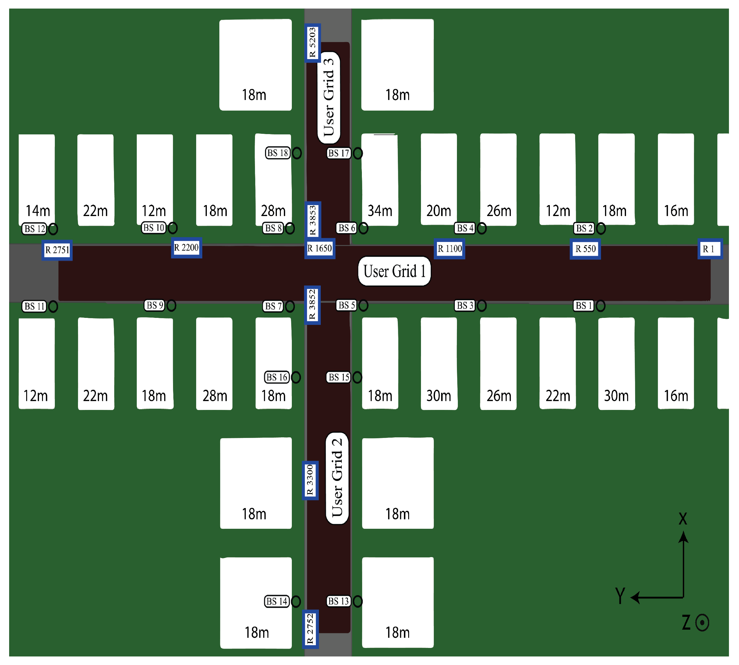
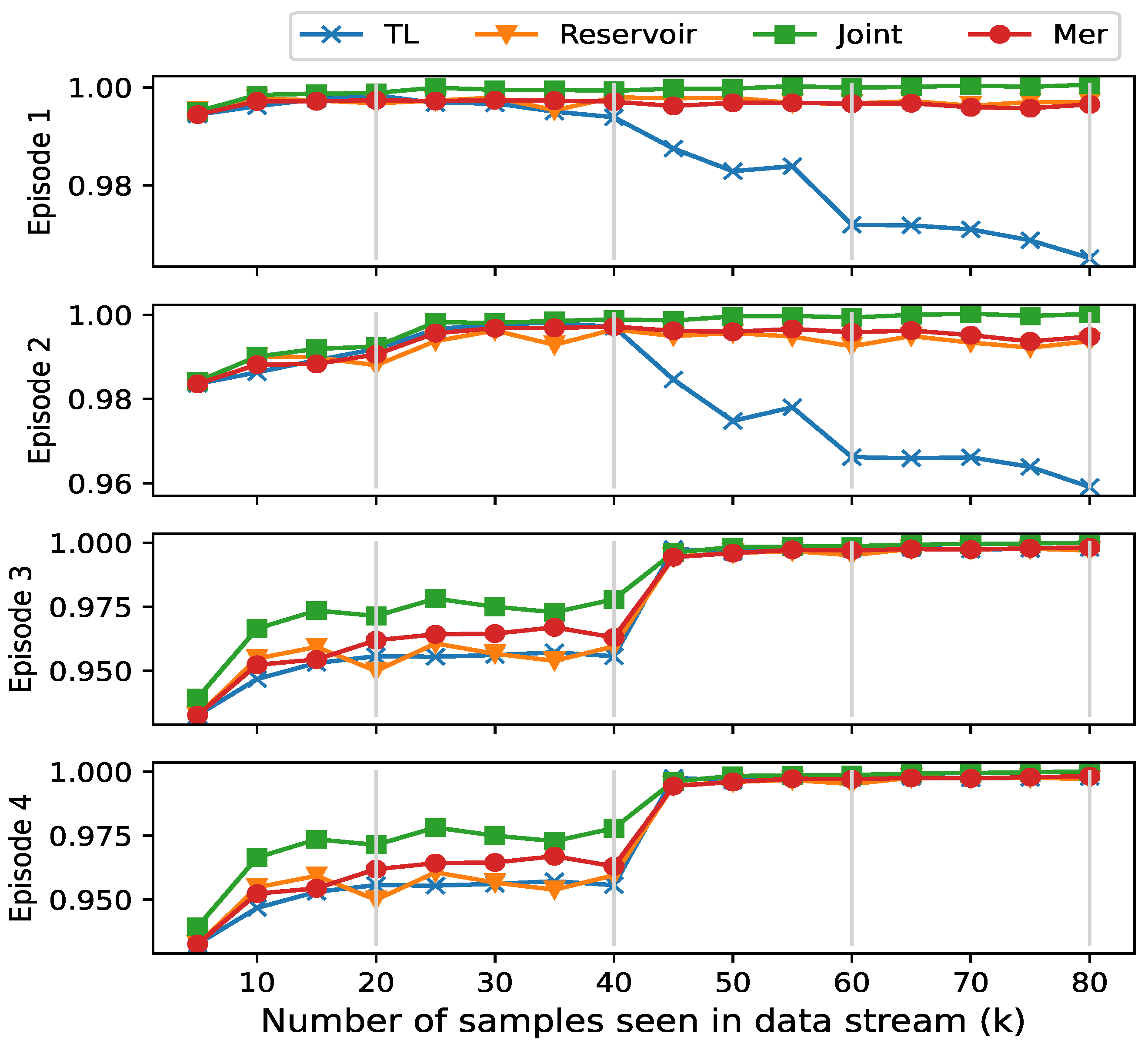
• Dataset Settings: The DeepMIMO dataset, generated by the Remcom Wireless Insite tool [46], is used to verify the effectiveness of our method through three distinct scenarios. As shown in Figure 6, in the DeepMIMO dataset, “O1_28” represents a specific simulation scenario. Specifically, “O1_28” is an outdoor environment at 28 GHz with two streets and an intersection. In this scenario, a total of 18 base stations (BS1-BS18) are deployed on both sides of the street, and the mobile users (MS) are located in three uniform x-y grids. Columns are indexed from C1 on the far right to C2751 on the far left. For each episode, 20,000 channel realizations are generated for training and 1000 for testing, derived from a configuration of 10 base stations with randomly selected K = 10 user positions from a predefined set. The scenarios are as follows: Episode 1 features UEs within rows 550 to 700 served by BS 1; Episode 2 has UEs within rows 800 to 1050, also served by BS 1; Episode 3 includes UEs within rows 1000 to 1250 served by BS 9; and Episode 4 involves UEs within rows 1300 to 1550 served by BS 9.

In this experiment, we compare the performance of four different training schemes in a dynamic environment. From Figure 7 and Figure 8, the experimental results show that the joint scheme performs the best in terms of performance and is able to quickly adapt to new training environments, but it suffers from the disadvantage of needing to accumulate data from all past training sessions, which leads to higher computational latency and memory consumption. In contrast, the MER scheme exhibits higher sum ratios while maintaining lower memory and time consumption, showing superior performance in adapting to new tasks. However, the TL scheme performs better in training scenarios, but the model is less adaptable to new environments, while the reservoir scheme leads to higher fluctuations in model performance due to its stochastic nature.

Taken together, despite its performance advantages, the joint scheme has high resource consumption and may not be suitable for resource-constrained environments. On the contrary, the MER scheme has a more balanced performance in terms of resource consumption and time efficiency and is better able to adapt to new tasks in a continuous learning environment while retaining the memory of old tasks. These findings emphasize the need to consider the trade-off between performance and resource consumption when designing training scenarios to ensure the feasibility and efficiency of the model in real-world applications. In addition, the experimental results also show that the meta-learning-based weight sharing dynamic optimization approach can effectively balance knowledge migration and interference between old and new tasks, thus achieving better model adaptation in a continuous learning environment.

In order to visually demonstrate the performance advantages of the MER algorithm in the real dynamic channel environment, 20 independent repeat experiments were carried out based on the DeepMIMO dataset, and the system compared MER with TL, reservoir, joint, and other baseline methods through rigorous non-parametric statistical tests.

Table 2. Real channel statistical test tables and analysis.

Method	Proposed	Reservoir	Joint	TL
Average Sum-rate	0.975	0.955	0.960	0.990
Standard Deviation	0.015	0.025	0.020	0.030
p-value	-	<0.001	0.003	0.012 s

quantitatively presents the performance differences of each algorithm in complex channel scenarios from three dimensions, mean-to-rate ratio, standard deviation, and statistical significance, so as to provide data support for evaluating the effectiveness of algorithms.

In terms of average and rate ratios, MER reached 0.975, significantly higher than TL’s 0.955 and reservoir’s 0.960 (p < 0.001 and p = 0.003), which verifies its performance superiority in dynamic channels. Although the average-to-rate ratio of the joint method is 0.990, it has a p-value of 0.012 with MER, which is close to the significance threshold, and combined with its memory consumption of 40 times that of MER (see Table 1), the overall price/performance ratio is not as good as that of MER. This shows that MER not only performs well in terms of performance but also in terms of resource efficiency.

In terms of stability, MER’s standard deviation is only 0.015, which is significantly lower than other methods, which means that its performance fluctuates less and is more robust in the face of complex situations such as channel mutations, such as rapid user movement and sudden obstruction of obstacles.

5. Conclusions

We propose a MER-based continuous learning beam prediction model to solve the beam formation adaptation problem in dynamic downlink MISO systems. It utilizes a meta-learning strategy to optimize the beam formation process and remembers historical data by means of an empirical playback method to achieve fast adaptation in a changing communication environment. It aims to address the problem of how to maintain model performance and achieve beam formation optimization in dynamically changing task assignments. We validate the performance of the proposed model in dynamic communication environments by conducting comparative experiments under randomly generated channel and real channel models. The results show that the model performs well in dealing with beam formation adaptation and rate maximization problems.

6. Future Work

In the current study, we have focused on the simulation of our proposed MER-based continuous learning beam prediction model, demonstrating its effectiveness in dynamic communication environments through extensive experiments. However, the practical deployment of such a model in real-world scenarios would require integration with actual hardware, such as FPGAs or GPUs, which are commonly used in base stations. This integration is crucial for ensuring the model’s real-time performance and computational efficiency.

Feasibility of Hardware Integration

The integration of our proposed model with actual hardware, such as FPGAs or GPUs, is a promising direction for future work. FPGAs offer high customization and parallel processing capabilities, making them suitable for real-time processing of complex algorithms like the ones used in our beam prediction model. GPUs, on the other hand, provide significant computational power and are well-suited for tasks that require massive parallel processing, such as deep learning and machine learning algorithms. By leveraging these hardware platforms, we can achieve low-latency and high-throughput processing, which are essential for dynamic beamforming in millimeter-wave (mmWave) communications. Future work will explore the practical implementation of our model on these hardware platforms, addressing challenges such as power efficiency, scalability, and real-time performance. This will involve optimizing the model’s architecture and training processes to ensure efficient deployment in resource-constrained environments, such as base stations. Additionally, we will investigate the use of hardware accelerators to further enhance the model’s performance and adaptability in dynamic communication scenarios.

References

1. Tariq, F.; Khandaker, M.R.; Wong, K.-K.; Imran, M.A.; Bennis, M.; Debbah, M. A speculative study on 6G. IEEE Wirel. Commun. 2020, 27, 118–125. [Google Scholar] [CrossRef]
2. Dai, G.; Huang, R.; Yuan, J.; Hu, Z.; Chen, L.; Lu, J.; Fan, T.; Wan, D.; Wen, M.; Hou, T.; et al. Towards Flawless Designs: Recent Progresses in Non-Orthogonal Multiple Access Technology. Electronics 2023, 12, 4577. [Google Scholar] [CrossRef]
3. Mao, B.; Liu, Y.; Guo, H.; Xun, Y.; Wang, J.; Liu, J.; Kato, N. On a hierarchical content caching and asynchronous updating scheme for non-terrestrial network-assisted connected automated vehicles. IEEE J. Sel. Areas Commun. 2025, 43, 64–74. [Google Scholar] [CrossRef]
4. Li, X.; Jin, S.; Suraweera, H.A.; Hou, J.; Gao, X. Statistical 3-D beamforming for large-scale MIMO downlink systems over Rician fading channels. IEEE Trans. Commun. 2016, 64, 1529–1543. [Google Scholar] [CrossRef]
5. Chen, S.; Gu, J.; Duan, W.; Wen, M.; Zhang, G.; Ho, P.-H. Hybrid Near-and Far-Field Communications for RIS-UAV System: Novel Beamfocusing Design. IEEE Trans. Intell. Transp. Syst. 2025, 1, 1–13. [Google Scholar] [CrossRef]
6. Cao, Y.; Maghsudi, S.; Ohtsuki, T.; Quek, T.Q.S. Mobility-aware routing and caching in small cell networks using federated learning. IEEE Trans. Commun. 2024, 72, 815–829. [Google Scholar] [CrossRef]
7. Yuan, Y.; Zhou, W.; Fan, M.; Wu, Q.; Zhang, K. Deformable Perfect Vortex Wave-Front Modulation Based on Geometric Metasurface in Microwave Regime. Chin. J. Electron. 2025, 34, 64–72. [Google Scholar] [CrossRef]
8. Ohtsuki, T. Machine learning in 6G wireless communications. IEICE Trans. Commun. 2023, 106, 75–83. [Google Scholar] [CrossRef]
9. Larsson, E.G.; Edfors, O.; Tufvesson, F.; Marzetta, T.L. Massive MIMO for next generation wireless systems. IEEE Commun. Magezine 2014, 52, 186–195. [Google Scholar] [CrossRef]
10. El Ayach, O.; Rajagopal, S.; Abu-Surra, S.; Pi, Z.; Heath, R.W. Spatially sparse precoding in millimeter wave MIMO systems. IEEE Trans. Wirel. Commun. 2014, 13, 1499–1513. [Google Scholar] [CrossRef]
11. Wang, T.; Wen, C.-K.; Wang, H.; Gao, F.; Jiang, T.; Jin, S. Deep learning for wireless physical layer: Opportunities and challenges. China Communucations 2017, 14, 92–111. [Google Scholar] [CrossRef]
12. Zhang, C.; Patras, P.; Haddadi, H. Deep learning in mobile and wireless networking: A survey. IEEE Commun. Surv. Tutor. 2019, 21, 2224–2287. [Google Scholar] [CrossRef]
13. He, H.; Wen, C.-K.; Jin, S.; Li, G.Y. Deep learning-based channel estimation for beamspace mmWave massive MIMO systems. IEEE Wirel. Commun. Lett. 2018, 7, 852–855. [Google Scholar] [CrossRef]
14. Liang, F.; Shen, C.; Wu, F. An iterative BP-CNN architecture for channel decoding. IEEE J. Sel. Top. Signal Process. 2018, 12, 144–159. [Google Scholar] [CrossRef]
15. Elbir, A.M.; Mishra, K.V.; Shankar, B.; Ottersten, B.E. A family of deep learning architectures for channel estimation and hybrid beamforming in multi-carrier mm-wave massive MIMO. IEEE Trans. Cogn. Commun. Netw. 2019, 8, 642–656. [Google Scholar] [CrossRef]
16. Elbir, A.M.; Papazafeiropoulos, A.K. Hybrid precoding for multiuser millimeter wave massive MIMO systems: A deep learning approach. IEEE Trans. Veh. Technol. 2020, 69, 552–563. [Google Scholar] [CrossRef]
17. Liang, F.; Shen, C.; Yu, W.; Wu, F. Towards optimal power control via ensembling deep neural networks. IEEE Trans. Commun. 2020, 68, 1760–1776. [Google Scholar] [CrossRef]
18. Sun, H.; Chen, X.; Shi, Q.; Hong, M.; Fu, X.; Sidiropoulos, N.D. Learning to optimize: Training deep neural networks for interference management. IEEE Trans. Signal Process. 2017, 66, 5438–5453. [Google Scholar] [CrossRef]
19. Hassan, S.U.; Mir, T.; Alamri, S.; Khan, N.A.; Mir, U. Machine Learning-Inspired Hybrid Precoding for HAP Massive MIMO Systems with Limited RF Chains. Electronics 2023, 12, 893. [Google Scholar] [CrossRef]
20. Zhang, T.; Dong, A.; Zhang, C.; Yu, J.; Qiu, J.; Li, S.; Zhou, Y. Hybrid Beamforming for MISO System via Convolutional Neural Network. Electronics 2022, 11, 2213. [Google Scholar] [CrossRef]
21. Echigo, H.; Cao, Y.; Bouazizi, M.; Ohtsuki, T. A deep learning-based low overhead beam selection in mmWave communications. IEEE Trans. Veh. Technol. 2021, 70, 682–691. [Google Scholar] [CrossRef]
22. Jang, S.; Lee, C. DNN-driven single-snapshot near-field localization for hybrid beamforming systems. IEEE Trans. Veh. Technol. 2024, 73, 10799–10804. [Google Scholar] [CrossRef]
23. Cao, Y.; Ohtsuki, T.; Maghsudi, S.; Quek, T.Q.S. Deep learning and image super-resolution-guided beam and power allocation for mmWave networks. IEEE Trans. Veh. Technol. 2023, 72, 15080–15085. [Google Scholar] [CrossRef]
24. Xia, W.; Zheng, G.; Zhu, Y.; Zhang, J.; Wang, J.; Petropulu, A.P. A deep learning framework for optimization of MISO downlink beamforming. IEEE Trans. Commun. 2020, 68, 1866–1880. [Google Scholar] [CrossRef]
25. Cao, Y.; Ohtsuki, T.; Quek, T.Q.S. Dual-ascent inspired transmit precoding for evolving multiple-access spatial modulation. IEEE Trans. Commun. 2020, 68, 6945–6961. [Google Scholar] [CrossRef]
26. Shen, Y.; Shi, Y.; Zhang, J.; Letaief, K.B. LORM: Learning to optimize for resource management in wireless networks with few training samples. IEEE Trans. Wirel. Commun. 2020, 19, 665–679. [Google Scholar] [CrossRef]
27. Zeng, J.; Sun, J.; Gui, G.; Adebisi, B.; Ohtsuki, T.; Gacanin, H.; Sari, H. Downlink CSI Feedback Algorithm With Deep Transfer Learning for FDD Massive MIMO Systems. IEEE Trans. Cogn. Commun. Netw. 2021, 7, 1253–1265. [Google Scholar] [CrossRef]
28. Zhang, B.; Li, H.; Liang, X.; Gu, X.; Zhang, L. Model Transmission-Based Online Updating Approach for Massive MIMO CSI Feedback. IEEE Commun. Lett. 2023, 27, 1609–1613. [Google Scholar] [CrossRef]
29. Cui, Y.; Guo, J.; Wen, C.-K.; Jin, S.; Han, S. Unsupervised Online Learning in Deep Learning-Based Massive MIMO CSI Feedback. IEEE Commun. Lett. 2022, 26, 2086–2090. [Google Scholar] [CrossRef]
30. Guo, J.; Zuo, Y.; Wen, C.-K.; Jin, S. User-Centric Online Gossip Training for Autoencoder-Based CSI Feedback. IEEE J. Sel. Top. Signal Process. 2022, 16, 559–572. [Google Scholar] [CrossRef]
31. Zhou, H.; Xia, W.; Zhao, H.; Zhang, J.; Ni, Y.; Zhu, H. Continual learning-based fast beamforming adaptation in downlink MISO systems. IEEE Wirel. Commun. Lett. 2023, 12, 36–39. [Google Scholar] [CrossRef]
32. Sun, H.; Pu, W.; Fu, X.; Chang, T.-H.; Hong, M. Learning to continuously optimize wireless resource in a dynamic environment: A bilevel optimization perspective. IEEE Trans. Signal Process. 2022, 70, 1900–1917. [Google Scholar] [CrossRef]
33. Sun, H.; Pu, W.; Zhu, M.; Fu, X.; Chang, T.-H.; Hong, M. Learning to Continuously Optimize Wireless Resource in Episodically Dynamic Environment. In Proceedings of the IEEE International Conference on Acoustics, Speech, and Signal Processing (ICASSP), Toronto, ON, Canada, 6–11 June 2021; pp. 4945–4949. [Google Scholar]
34. Isele, D.; Cosgun, A. Selective experience replay for lifelong learning. In Proceedings of the Thirty-Second AAAI Conference on Artificial Intelligence, New Orleans, LA, USA, 2–7 February 2018; pp. 226–231. [Google Scholar]
35. Cao, Y.; Lu, W.; Ohtsuki, T.; Maghsudi, S.; Jiang, X.-Q.; Tsimenidis, C. Memristor-based meta-learning for fast mmWave beam prediction in non-stationary environments. arXiv 2025, arXiv:2502.09244. [Google Scholar]
36. Lyu, M.; Ng, B.K.; Lam, C.-T. Downlink beamforming prediction in MISO system using meta learning and unsupervised learning. In Proceedings of the ICCT, Wuxi, China, 20–22 October 2023; pp. 188–194. [Google Scholar]
37. Lopez-Paz, D.; Ranzato, M. Gradient Episodic Memory for Continual Learning. In Proceedings of the 31st Annual Conference on Neural Information Processing Systems, Long Beach, CA, USA, 4–9 December 2017. [Google Scholar]
38. Chaudhry, A.; Dokania, P.K.; Ajanthan, T.; Torr, P.H. Riemannian Walk for Incremental Learning: Understanding Forgetting and Intransigence. arXiv 2018, arXiv:1801.10112. [Google Scholar]
39. Hintze, A. The role weights play in catastrophic forgetting. In Proceedings of the 2021 8th International Conference on Soft Computing & Machine Intelligence (ISCMI), Cario, Egypt, 26–27 November 2021; pp. 160–166. [Google Scholar]
40. Masarczyk, W.; Tautkute, I. Reducing catastrophic forgetting with learning on synthetic data. In Proceedings of the 2020 IEEE/CVF Conference on Computer Vision and Pattern Recognition Workshops (CVPRW), Seattle, WA, USA, 14–19 June 2020; pp. 1019–1024. [Google Scholar]
41. Zhang, M.; Li, H.; Pan, S.; Chang, X.; Zhou, C.; Ge, Z.; Su, S. One-shot neural architecture search: Maximising diversity to overcome catastrophic forgetting. IEEE Trans. Pattern Anal. Mach. Intell. 2021, 43, 2921–2935. [Google Scholar] [CrossRef]
42. Riemer, M.; Cases, I.; Ajemian, R.; Liu, M.; Rish, I.; Tu, Y.; Tesauro, G. Learning to learn without forgetting by maximizing transfer and minimizing interference. arXiv 2018, arXiv:1810.11910. [Google Scholar]
43. Lahiri, S.; Ganguli, S. A memory frontier for complex synapses. In Proceedings of the NeurIPS, Lake Tahoe, NV, USA, 5–10 December 2013; pp. 1034–1042. [Google Scholar]
44. Finn, C.; Abbeel, P.; Levine, S. Model-agnostic meta-learning for fast adaptation of deep networks. In Proceedings of the ICML, Sydney, NSW, Australia, 6–11 August 2017; pp. 1126–1135. [Google Scholar]
45. Nichol, A.; Schulman, J. Reptile: A scalable metalearning algorithm. arXiv 2018, arXiv:1803.02999. [Google Scholar]
46. Alkhateeb, A. DeepMIMO: A generic deep learning dataset for millimeter wave and massive MIMO applications. In Proceedings of the Information Theory and Applications Workshop (ITA), San Diego, CA, USA, 10–15 February 2019. [Google Scholar]
Figure 1. A dynamic channel distribution scenario where different data follow different distributions and the set of data collected in each time period t is denoted as D t .
Electronics 14 02734 g001
Figure 2. (A) The stability–plasticity dilemma focuses on how to maintain network stability to preserve old knowledge while allowing the network to remain sufficiently plastic with respect to current learning content. The transfer–interference trade-off further extends this dilemma by considering not only the impact on past knowledge but also the impact of weight sharing on future knowledge acquisition during the learning process. This trade-off perspective is critical because simply reducing weight sharing may not be sufficient to support effective knowledge transfer in future learning. (B) demonstrates the concept of knowledge transfer in weight space, where weight updates during the learning process can mutually reinforce each other and enhance existing learning outcomes. (C) depicts the phenomenon of interference in weight space, illustrating how weight updates during the learning process may interfere with each other, leading to the forgetting or impairment of existing learning outcomes.
Electronics 14 02734 g002
Figure 3. MER algorithm model.
Electronics 14 02734 g003
Figure 4. Average sum ratios of different training scenarios across all episodes for different schemes.
Electronics 14 02734 g004
Figure 5. Sum ratios of different training scenarios per episode between different scenarios.
Electronics 14 02734 g005
Figure 6. “O1_28” an outdoor scenario of two streets and one intersection at operating frequencies of 28 GHz in DeepMIMO version v3.
Electronics 14 02734 g006
Figure 7. Average sum ratios of different training scenarios across all episodes for different schemes.
Electronics 14 02734 g007
Figure 8. Sum ratios of different training scenarios per episode between different scenarios.
Electronics 14 02734 g008