A K-Means Approach to Temperature Estimation in Non-Linear Power Inductors

Abstract

The temperature of a power inductor operated up to saturation in a DC/DC converter is estimated based on its current profile. A dataset built by a proper model of the non-linear inductor was generated, reproducing its current profiles in different operating points. The measured current waveform is compared with the dataset values. The K-means classification is adopted to obtain clusters characterizing the operation in saturation, in which a precise estimation can be carried out. The linear and the deep saturation zones give poor information about the temperature; on the other hand, the temperature evaluation is of interest up to saturation. The K-means clustering allows for a relevant reduction in the computational effort. The proposed approach avoids direct measurement of the current by dedicated sensing; the temperature can be forecast before reaching the steady state, enhancing the converter’s reliability. Finally, experimental tests are used to assess the goodness of the proposed method.

1. Introduction

Power inductors are crucial in the operation of Switched-Mode Power Supplies (SMPS); they store and release energy according to the converter’s switching frequency. A magnetic core boosts the inductance, but it also increases weight and size, allowing the power density to be lowered [1,2]. The magnetic material introduces a dependency of the inductance on the current; however, the traditional exploitation of a power inductor considers, as the operating zone, the current interval in which a maximum decrease of 10% from the rated value obtained with a small current occurs [3]. Within this interval, the inductance can be considered constant. A more recent approach considers the extension of the current interval up to the value at which the rated inductance is reduced by 50%; this threshold is named the saturation value [4,5]; in this way, a smaller and cheaper inductor can be used, improving power density. This extension raises some issues. First of all, the current flowing through the inductor is non-linear, showing a cusp-like shape instead of the well-known triangular waveform [6,7]; as a consequence, a higher current peak flows through the inductor and the series connected components like the power MOSFET [8,9]. Moreover, due to the modified current shape, its spectrum contains more harmonics requiring suitable filtering [10,11], losses are increased, leading to a higher operating temperature of the core, and the behavior of the magnetic core must be considered as a function of the temperature, potentially causing a thermal runaway [8,12].

These issues can be addressed during the design with a suitable inductor model considering the inductance vs. the current with the temperature as a parameter [13,14,15,16]. A relevant feature encompassed in the current shape, particularly concerning the temperature, is extracted in this paper by the K-means clustering method. There has been a growing interest in clustering techniques in power applications. As an example, the authors of [17] exploit clustering to define self-efficiency maps for prosumers, equipped with a hybrid photovoltaic-battery energy storage system (PV-BESS), based on their self-sufficiency expectations. In [18], K-means clustering is emphasized as a well-recognized and frequently used algorithm in modern power systems such as forecasting in wind power management [19], and solar energy [20], or in power transmission and management [21]. Finally, the paper [22] proposes clustering applied to environmental conditions based on their impact on the power electronics reliability.

The current waveform through a non-linear power inductor needs a suitable model to be properly reproduced. The literature proposes different models taking into account the core temperature as well. The literature proposes two main models dedicated to power inductors operated up to saturation, considering the core temperature as well. The first model is based on the shape of the arctangent curve; this curve also shows a continuous derivative. The identification of this model is based on the knowledge of four coefficients corresponding to the inductance values measured at low current, to the drop of the nominal inductance of 30% and 70%, and to the deep saturation value [4,23]. The latter model exploits a third-order curve. The model can be identified based on the same parameters as the Arctan model; however, better results can be retrieved by an augmented dataset obtained by a measurement system. A comparison between these two models shows that both models can reproduce the inductance curve when the current approaches saturation, which represents the main operating region. The polynomial model reproduces the increase in the inductance when the current increases from low values, but it cannot reproduce the behavior after the deep saturation point. The arctan model exhibits a slightly decreasing trend when the current increases from a small value, but the deep saturation behavior is also well reproduced for higher currents [24]. In order to overcome these issues, a new model is proposed in this paper. The key issue is knowledge of the temperature of the power inductor core as the control algorithms designed for SMPS exploiting the saturating inductor, such as the Quasi-Constant On-Time Control, could require the temperature as an input [25]. A dedicated sensor can acquire this parameter, increasing the overall cost. In principle, the temperature can be calculated based on losses [26,27,28], and on the thermal constant of the inductor [12]; unfortunately, losses are difficult to estimate precisely, particularly concerning magnetic losses, since the Steinmetz formulas would require suitable coefficients taking into account the non-sinusoidal waveforms [29,30,31,32].

The method proposed in this paper is based on a dataset built by simulation containing the waveforms of the currents flowing through an inductor in a DC/DC converter. The current sampled in the real converter is compared with the waveforms of the dataset once the mean square error (MSE) is minimized. The K-means classification reduces the computational effort to achieve clusters characterizing the operation in which a precise estimation can be carried out. The novel contributions of the paper are as follows: (a) a new model of aq power inductor is proposed overcoming the limitations of those proposed in the literature, and (b) clustering, which allows for reduction in the computational effort.

The paper is organized as follows: After the introduction, which summarizes the main issues concerning the modeling of power inductors and temperature estimation, the new model is explained in Section 2. Section 3 explains the structure of the converter adopted for simulation and retrieving the experimental data. Section 4 describes how the dataset has been obtained by implementing the DC/DC converter with the proposed model. Section 5 presents the data clustering by K-means. Section 6 describes the experimental test rig. Finally, some tests are proposed in Section 7, considering different operating points to show the advantages of the proposed approach.

2. Non-Linear Inductor Modeling

A linear inductor is an electrical component characterized by a differential equation where the voltage at its terminals is proportional to the current derivative, as described by Equation (1). The proportionality constant is called the inductance L. In a linear inductor, the inductance is constant.

$$V_L=L{\displaystyle \frac{di}{dt}}$$

(1)

The inductors are formed by a metallic coil, typically copper, wound on a magnetic core. Different materials are adopted for the magnetic core depending on the application; in the power electronic field, ferrite cores are preferred due to their low losses and high magnetic permeability, which ranges from 1 × ${10}^3$ to 20 × ${10}^3$, and deep saturation, which ranges from 0.25 T to 0.45 T [33,34,35]. The magnetic core allows an increase in inductance while maintaining a low size; however, it introduces an inductance that lowers the current. This inductance variation represents a non-linear behavior that is highly temperature-dependent. Usually, the inductors are exploited within the range of current such that the inductance remains constant (up to 10% of the inductance drop) and the behavior of the inductor is linear as expressed in (1). By exceeding this range, the inductance is heavily reduced, and the inductor current waveform results in a distorted cusp-like waveform.

The inductors’ non-linear behavior is characterized by an inductance value that depends on the current and the core temperature, $T_{core}$, as in Equation (2):

$$V_L=L(i,T_{core}){\displaystyle \frac{di}{dt}}$$

(2)

Such behavior impacts the performance of the DC-DC converter, since it introduces a higher current peak that stresses the switches. Therefore, a thorough analysis of the converter implementing such an inductor is needed when exploiting the inductors in the non-linear range. A proper inductor model is essential for this purpose. For this reason, many behavioral inductor models have been proposed in the literature [4,6,8,24,25,36,37,38,39].

The inductor vs. current characteristics are sigmoid, with a region at low current where the inductance is practically constant to the nominal value, a region of deep saturation where the inductance is constant but at a value much lower than the nominal value, and an in-between transition in which the inductance value corresponding to one half of the nominal value (called the saturation point) is located.

A new behavioral model is presented; it is based on the generalized logistic curve, which is used in a variety of fields to model s-shape behaviors. The analytical expression of the inductance is given by:

$$L\left(i\right)=L_{nom}-{\displaystyle \frac{L_{nom}-L_{deep}}{1+\exp [-\gamma (i-I_0)]}}$$

(3)

where $L_{nom}$ is the nominal inductance, $L_{deep}$ is the inductance value at deep saturation, $\gamma$, which in this context is positive, represents the decline rate of the inductance, and $I_0$ is the current value at which the inductance reach its inflection point, defined as $(L_{nom}+L_{deep})/2$. This inductance behavioral model is also temperature-dependent through the parameters $L_{nom}$, $L_{deep}$, $\gamma$, and $I_0$. The temperature-dependency of the parameters for an inductor model can be assumed to be linear [40,41] as follows:

$$L_{nom}\left(T_{core}\right)=L_{nom,0}+L_{nom,1}·T_{core}$$

(4)

$$L_{deep}\left(T_{core}\right)=L_{deep,0}+L_{deep,1}·T_{core}$$

(5)

$$\gamma \left(T_{core}\right)={\gamma }_0+{\gamma }_1·T_{core}$$

(6)

$$I_0\left(T_{core}\right)=I_{0,0}+I_{0,1}·T_{core}$$

(7)

This model is composed of two terms—a first term that gives the nominal value and a second term that addresses the non-linearity given by the saturation. The model exhibits two main advantages with respect to other assessed models such as the polynomial and the arctangent models: (i) the proposed expression is a sigmoid function that is capable of reproducing the overall inductance characteristics from the linear region to the deep saturation region (contrary to the polynomial expansion), and (ii) its expression is simpler than the arctangent model so the magnetic flux is easily achievable by integrating the inductance as a function of the current and setting the zero flux condition at zero current:

$$\mathrm{\Phi }=L_{nom}·i-{\displaystyle \frac{L_{nom}-L_{deep}}{\gamma }}\log \left[{\displaystyle \frac{1+\exp \left(\gamma (i-I_0)\right)}{1+\exp (-\gamma ·I_0)}}\right]$$

(8)

Remarkably, the expression of the magnetic flux $\mathrm{\Phi }$ given by (8) is composed of a term that is linearly dependent on the nominal current (linear regime) and by a non-linear term that includes the saturation of the core. This function describes a continuous and differentiable curve that approximates linear flux behavior with slope $L_{nom}$ for current $i\ll I_0$ and transitions smoothly to linear behavior with slope $L_{deep}$ for $i\gg I_0$. 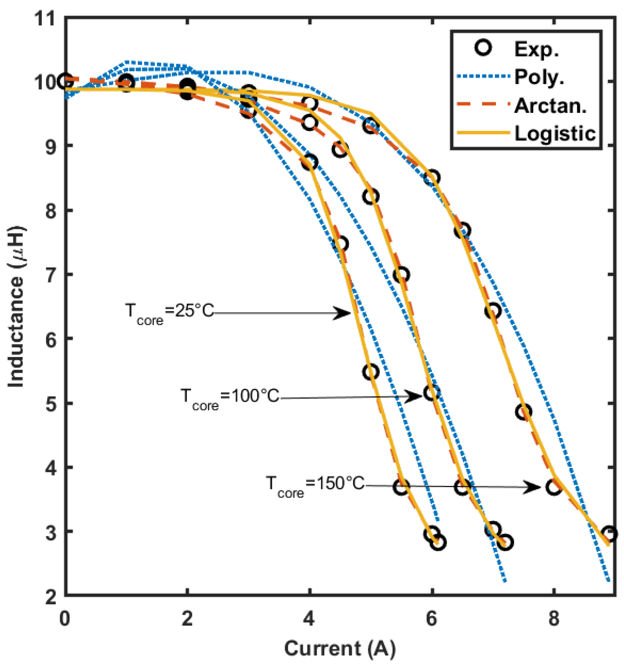The parameter $I_0$ defines the center of the transition, while $\gamma$ controls its sharpness: larger values of $\gamma$ produce a steeper transition between the two linear regimes. A quantitative comparison was carried out to assess the performance of the proposed logistic-based inductor model against a third-order polynomial fit and an arctangent-based model, which are commonly adopted to represent non-linear magnetic behavior. The evaluation was based on the root mean square error (RMSE) between the model output and the experimental inductance values over the full current range. The comparison was performed using the characterization data of the MSS1246-103 inductor from Coilcraft, UK, Europe [42] within a temperature range from 25 °C to 150 °C. The resulting RMSE was 0.5076 for the polynomial model, 0.05870 for the arctangent model, and 0.1172 for the proposed logistic model. A graphical comparison is provided in Figure 1, where the model responses are plotted against the experimental data at 25 °C, 100 °C, and 150 °C. Furthermore, unlike the polynomial approach, it accurately captures both the linear and saturation regions. As previously stated, the logistic model also allows for direct and smooth computation of the magnetic flux via integration, which is advantageous for subsequent analytical developments.

The data needed for modeling (3) can be retrieved from the power inductors datasheet, which includes information regarding the reduction in the inductance with current. Manufacturers often define the saturation current differently, e.g., with the current at which the inductance is reduced by 10%, 20% or 30% without a common standard and rarely showing the value of inductance at complete saturation (deep saturation) and the temperature dependency; therefore, power electronic engineers rely on laboratory testing to evaluate the full inductance vs. current curve, also including the temperature [43].

3. The Converter Under Study

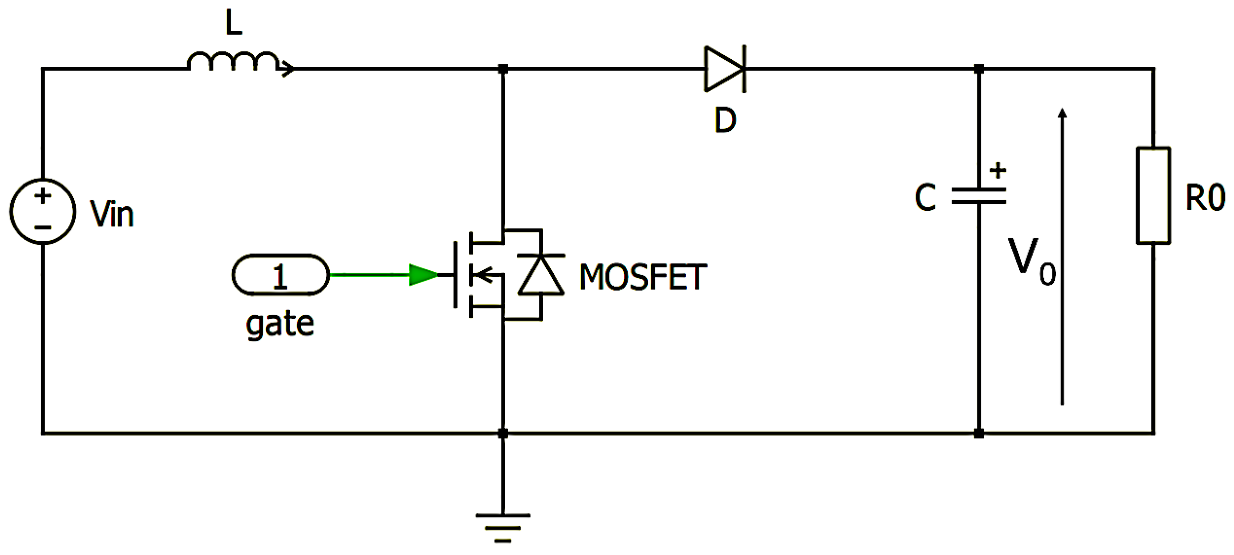
The non-linear inductor was tested as a component of a DC/DC boost converter, which is described in this section. The boost converter is classified as a transformerless, single-inductor, step-up DC-DC converter. The circuit layout does not involve a transformer, meaning the input and output sections share a common ground. The circuit exploits only one inductor, which serves as the energy transfer element of the SMPS. Furthermore, the boost converter can only generate an output voltage value higher than the input voltage value, thus boosting the input voltage to the desired output voltage. The inductor current represents the input current of the boost converter.

To properly reproduce the inductor behavior, the model is crucial; it must be enclosed in the converter simulation. The Equation (3) was implemented to obtain the current waveforms varying the temperature. Figure 2 shows an example of inductance versus the inductor current under different operating temperature conditions based on Equation (3). In the linear region, the inductance is almost constant at the nominal value $L_{nom}$; the inductance defines the boundary of this region, which drops to 90% of its nominal value. Increasing the current, the power inductor enters the weak saturation region; at saturation, the inductance is reduced to 50%, then the inductance value drops to 10 ÷ 20% of its nominal value, reaching the so-called deep saturation region. For such current values, the inductor is almost constant between 10% and 20% of its nominal value ($L_{deep}$). By varying the operating temperature, the nominal and the deep saturation inductance slightly vary; by contrast, relevant variations occur in the intermediate regions [4].

Figure 3 shows the boost converter circuit, including the ideal components. The common node between the power inductor, the MOSFET, and the power diode is usually referred to as the switching node.

By assuming a constant switching frequency control, a square-wave signal with constant period ($T_{sw}$) and variable duty cycle (d) serves as the MOSFET gate drive signal, dictating the length of the converter sub-periods $T_{on}$ and $T_{off}$ and, consequently, the input–output gain. Assuming constant input voltage $V_{in}$, constant duty cycle D, and constant power load R, the analysis is carried out under steady-state conditions. The sub-period $T_{on}$ corresponds to the MOSFET conduction sub-period. The on-time, by definition of the duty-cycle d, is given by:

$$T_{on}=d·T_{sw}$$

(9)

The analysis assumes that only two states per switching cycle exist, corresponding to the so-called continuous conduction mode of operation. Therefore, the $T_{off}$ period is given by:

$$T_{off}=T_{sw}-T_{on}=(1-d)·T_{sw}$$

(10)

When the MOSFET is turned on, it ideally behaves as a short-circuit, thus clamping the switching node to ground. Since a positive output voltage is generated, the diode is reverse-biased throughout the sub-period, thus ideally acting as an open circuit. The equivalent circuit during $T_{on}$ is shown in Figure 4a.

During $T_{on}$, the inductor is connected in parallel to the constant positive input and stores energy from the input source. During the on-time, the voltage across the inductor is given by:

$$v_{L,on}=V_{in}$$

(11)

Considering the constitutive equation of the inductive dipole, as given by (12), a linear increase in the power inductor current occurs during the on-time, corresponding to energy storage.

$$v_L=L{\displaystyle \frac{di}{dt}}$$

(12)

During the on-time, the output capacitor supplies the constant current required by the power load, which is modeled by a resistor.

When the MOSFET is turned off, thus equivalent to an open circuit, the inductor, resisting the potential current interruption, compels the diode to turn on. Then, the diode is forced into conduction by the inductor current. During the $T_{off}$, the MOSFET acts as an open circuit and the ideal diode as a short-circuit, as shown in Figure 4b.

The inductor is now connected between the input and output, releasing the previously stored energy to the output section. The inductor voltage is now given by:

$$v_{L,off}=V_{in}-V_o$$

(13)

Under steady-state conditions, the energy stored during the on-time by the power inductor is counterbalanced by the energy released. Therefore, the energy stored during the on-time should equal the energy released during the off-time. Otherwise, a net variation in the stored energy occurs, thus violating the steady-state assumption. Therefore, during the off-time, an inductor current decrease occurs, induced by a constant negative inductor voltage, thus meaning that the output voltage is always higher than the input voltage according to Equation (13).

The inductor current variation $\Delta I_L$ in a period $\Delta T$ can be calculated from the constitutive equation of the inductor, as given by:

$$\Delta I_L={\displaystyle \frac{V_L}{L}}\Delta T$$

(14)

The output voltage equation is given by equating the current increase during the on-time and the current decrease during the off-time.

$$\Delta I_{L,on}={\displaystyle \frac{V_{in}D{T}_{sw}}{L}}=\left|\Delta I_{L,off}\right|={\displaystyle \frac{(V_o-V_{in})(1-D)T_{sw}}{L}}$$

(15)

By Equation (15), the input–output relationship (16) is obtained.

$$V_o={\displaystyle \frac{V_{in}}{1-D}}$$

(16)

Since D ranges from 0 to 1, the output voltage is always higher than the input voltage. This relationship equates the output voltage to the input voltage as D approaches zero. The ratio between the output and the input voltage increases ideally unbounded as D approaches one.

Since steady-state conditions are assumed, the average capacitor current over one switching cycle equals zero. Consequently, the average diode current over one switching cycle must equal the load current. The diode current is zero during the on-time, whereas during the off-time, the diode current is equal to the inductor current. Consequently, the relationship between the input (inductor) current and the output current is given by (17).

$$I_{D,\mathrm{avg}}=I_{L,\mathrm{avg}}{\displaystyle \frac{T_{off}}{T_{sw}}}=I_{L,\mathrm{avg}}(1-D)=I_{out}$$

(17)

From Equation (17), Equation (18) is given.

$$I_{L,\mathrm{avg}}={\displaystyle \frac{I_{out}}{1-D}}$$

(18)

By taking into account the constitutive equation of the capacitor (Equation (19)), assuming steady-state operating conditions, and keeping in mind that the modulus of the capacitor current is equal to the load current throughout the on-time, the output voltage ripple can be obtained by Equation (20).

$$i_c=C{\displaystyle \frac{d{v}_c}{dt}}$$

(19)

$$\Delta V_o={\displaystyle \frac{I_{out}{T}_{on}}{C}}={\displaystyle \frac{I_{out}D{T}_{sw}}{C}}$$

(20)

A boost converter with parameters listed in the

Table 1. The parameters in the dataset.

Symbol	Units	Description	Values Range
$V_{in}^{*}$	[V]	Input supply voltage	$9–20$
$R^{*}$	[$\mathrm{\Omega }$]	Load resistance	$4–30$
C	[$\mathsf{\mu }$F]	Output capacitance	1000
$V_f$	[V]	Diode drop forward voltage	1
$r_C$	[$\mathrm{\Omega }$]	Parasitic resistance of output capacitance	$0.05$
$r_L$	[$\mathrm{\Omega }$]	Parasitic resistance of inductor	$0.04$
$r_{DS}$	[$\mathrm{\Omega }$]	MOSFET conduction resistance	$0.0042$
$T_{sw}$	[s]	Switching period	$4\times {10}^{-6}$
$D^{*}$	-	Duty cycle	-
$T_{core}$	[ °C]	Inductor core temperature	$25–150$
$T_{camp}$	[s]	Sampling time	$2\times {10}^{-7}$
$V_o$	[V]	Output voltage	24
$i_L^{*}$	[A]	Inductor current (20 samples)	-
L	[H]	Inductance (20 samples)	-

* These values vary according to the operating conditions.

was simulated in the MATLAB^® R2024b/Simulink environment; this allows a dataset to be retrieved. An example of simulation obtained with $V_{in}=$ 12 V, $D=$ 0.5, $R=$30 $\mathrm{\Omega }$, assuming a constant inductance of 10 μH, is shown in Figure 5. It can be noted that a constant inductance original triangular waveform is produced. Using the non-linear model of the inductor including the temperature, as shown in Figure 6, a cusp-like waveform of the inductor current is obtained. The parameters of Equations (4)–(7) needed for the implementation of the model (3) are given in

Table 2. The parameters for the inductor model.

Parameter	Value
$L_{nom,0}$	$10\times {10}^{-6}$
$L_{nom,1}$	0
$L_{deep,0}$	$2\times {10}^{-6}$
$L_{deep,1}$	0
${\gamma }_0$	$1.178$
${\gamma }_1$	$4.547\times {10}^{-3}$
$I_{0,0}$	$7.558$
$I_{0,1}$	$-1.790\times {10}^{-2}$

. It should be noted that the temperature dependency of $L_{nom}$ and $L_{deep}$ has been neglected and the corresponding temperature coefficients have been set to zero.

In Figure 5a, from the top to the bottom screen, the gate drive signal, the inductor current, and the output voltage waveforms are shown. The $T_{on}$ and $T_{off}$ periods are highlighted in the figure. According to Equation (16), the average output voltage value equals 24 V, double the input voltage. The measured ripple voltage is equal to 16 mV, according to Equation (20). The load current equals 0.8 A and the average inductor current equals 1.6 A, according to Equation (18). The inductor current ripple is equal to 2.4 A, according to Equation (15).

Figure 5b shows, from the top to the bottom screen, the gate drive signal, the inductor current, the MOSFET current, the diode current, and the capacitor current waveforms. The MOSFET current is equal to the inductor current during the on-time, whereas it is equal to zero during the off-time. The diode current is equal to the inductor current during the off-time, whereas it is equal to zero during the on-time. The capacitor current is equal to the diode current waveform shifted towards negative values by the load current value. In fact, during the on-time, the capacitor entirely supplies (a negative value according to the passive dipole sign convention) the load current, whereas during the off-time, it is equal to the difference between the diode current and the load current, according to Kirchhoff’s current law, at the output node.

The current ripple does not depend on the load current. If the load current decreases, the inductor current waveform is strictly shifted towards lower average values. Yet, a critical point exists where the inductor current’s minimum value equals zero. At this point, any further decrease in the load current leads to the diode interdiction during the off-time. Consequently, until the next on-time, neither the MOSFET nor the diode conducts, and the inductor current is maintained at zero value. This condition corresponds to the so-called discontinuous conduction mode of operation. The switching period is now divided into three parts: the on-time, where the MOSFET is turned-on and the diode is reverse-biased, the off-time, where the diode is turned on and the MOSFET is turned off, and the so-called dead time, where neither the MOSFET nor the diode are in the conductive state and the inductor current is constant at a zero value. The analysis in the discontinuous conduction mode is more complex than in the continuous conduction mode, and the output relationship depends on the switching frequency, the power inductor, the power load, and the input voltage and duty cycle. A continuous conduction mode is provided for all converter operating conditions to prevent the complexity of the analysis from increasing. For this paper, the waveforms corresponding to the current flowing through the inductor are acquired with the main operating parameters of the converter, building the dataset.

4. Simulation and Dataset Building

The dataset is built by simulation, aiming to reproduce different working conditions and exploiting the power inductor from the linear behavior exhibited at low currents, passing through the operation in saturation where the non-linear behavior is solicited, up to deep saturation where the inductance is linear again but showing a value much lower compared with the rated one. From the curves describing the inductance versus current as reported in Figure 6, obtained with a real inductor (delivered by Coilcraft, model MSS1246-103), it can be noted that the curves are superimposed both for low and high currents. As a consequence, low accuracy of the temperature estimation is expected in these regions. On the other hand, in regions with low currents, the temperature does not show an appreciable increase from the environment. Moreover, deep saturation, occurring for higher currents, is not of practical interest due to the high current potentially affecting the other components of the converter. This issue is faced with clustering, allowing for identifying regions in which good accuracy can be retrieved and avoiding regions where the temperature has poor interest. This situation is depicted in Figure 7, where three different subsets of inductor current waveforms are shown for different operating temperature values, ranging from 25 °C to 150 °C. The current waveforms are retrieved with the same operating input voltage and duty-cycle, corresponding to $V_{in}=12\mathrm{V}$ and $D=50\%$. In contrast, the load resistance varies the load current since it is proportional to the average current flowing through the inductor according to Equation (18). The behavior in the linear region is shown in Figure 7a. The inductance value is nearly constant with varying operating temperature conditions; consequently, the boost inductor current is triangular, and the temperature value does not significantly affect the current waveform. In Figure 7c, the full deep saturation region, for extremely high current values, is shown. The inductance value is almost constant at the deep saturation value $L_{deep}$. Consequently, a triangular inductor current waveform is expected. If the current ripple is sufficiently high, the non-linear power inductor goes through the weak saturation region at the lowest ripple current values, according to the corresponding temperature curve. Compared to high-temperature curves, the effect is more pronounced at low temperatures, where the deep saturation current limit is higher and the weak saturation steepness is lower. As shown in Figure 7b, the inductor current crosses the linear region towards the weak saturation region for intermediate currents. The temperature has a significant impact on the non-linear inductor behavior. At 25 °C, the steepness is low and the weak saturation current limit is high. As a result, the non-linear impact might not be noticeable. However, at 150 °C, the inductor current is heavily distorted by the non-linearities of the power inductor. The peak current rises as the temperature rises because, under the same operating conditions for the input voltage, duty cycle, and output current, the limit current of the weak saturation region decreases, and the steepness increases. In conclusion, the temperature estimation can be accurately retrieved when the non-linear inductor behavior is exploited, corresponding to the curves of Figure 7b. This is of practical interest in power converters.

The dataset contains 4368 samples, represented as rows, each containing the parameters shown in Table 1. The table shows three kinds of parameters as follows: the fixed parameter of the circuit, which represents the circuit components ($C,V_f,r_C,r_L,r_{DS},T_s,V_o$) or the simulation parameter $T_{camp}$; parameters imposed for the different operating conditions ($V_{in},R,D,T_{core}$); and parameters varying during the switching period for given operating conditions ($i_L,L$). The output voltage $V_o$ is kept constant by the converter’s feedback. The current and the inductance are sampled during the switching period to provide 20 samples.

The clustering method, explained in the next section, aims to consider only this reduced dataset, reducing the computational burden of a searching algorithm.

5. Methods: Dataset and Clustering

Clustering is the task of grouping a set of objects using similarity criteria that involve measuring defined characteristics. According to these criteria, objects in the same cluster should be more similar to each other than objects belonging to different clusters. Usually, these characteristics are measurable and are converted into numbers; in this case, the similarity can be transformed into a metric distance (e.g., Euclidean distance or Manhattan distance). Clustering algorithms are developed to achieve this grouping automatically and efficiently. Usually, these algorithms have some parameters that need to be adjusted.

One of the simplest clustering algorithms is the so-called K-means, which starts with a predefined number of cluster centers, called centroids, randomly positioned concerning the set of objects, called samples, to group $x_i\in Xi=1,2,\dots ,N$. Each centroid ${\mu }_{j}j=1,2,\dots ,K$ is distinct from the samples but in the same space. The presence of the K centroids separates the objects into K clusters $C_j$, where:

$$\left\{x_i\in C_j\mathrm{if}d(x_i,{\mu }_j)<d(x_i,{\mu }_l)\forall {\mu }_l\mathrm{with}l\ne j\right\}$$

(21)

The K-means clustering algorithm is based on the following steps:

• assign the sample $x_i$ to the cluster using Equation (21)
• update the position of the centroids using the following equation:

  $${\mu }_j^{(t+1)}={\displaystyle \frac{1}{|C_j^{\left(t\right)}|}}\sum _{x_i\in C_j}{x}_i$$

  (22)

where $|C_j|$ is the number of samples in $C_j$.

The algorithm tries to minimize the following equation:

$$\arg \underset{C_j}{\min }\sum _{j=1}^K\sum _{x_i\in C_j}\left|\right|x_i-{\mu }_j{\left|\right|}^2$$

(23)

where ${\mu }_j$ is given in Equation (22).

Usually, the ${\mu }_j$ are initialized with some random sample values. The algorithm does not guarantee convergence to the global minimum.

One application of the K-means algorithm is vector quantization, which involves dividing a large set of points into groups, each represented by its centroid.

In the K-means clustering algorithm, the only parameter to decide is the number of clusters. This decision requires prior knowledge about the number of clusters that could be in the dataset or some knowledge about the physical phenomena under observation. There are some techniques, e.g., the calculation of silhouette coefficients, that help in the selection of the K value; the investigation of this value for the clustering is presented in Appendix A. When the appropriate number of clusters is decided, the clustering algorithm is started using a random initial position of the cluster centers. The obtained position of the cluster centers is the algorithm’s output. Due to the random initialization of the position of the cluster centers in the clustering space, this output can also be different among the trials. In this study, we decided to use the $i_{L\max }$ as the input variable for the clustering algorithm. In our case, we need to separate three specific situations: linear behaviors of the inductor, and consequently, linear variations of the current, as indicated in Figure 7a; linear variation of the $i_L$ due to the saturation of the inductor, as indicated in Figure 7c; and the non-linear phenomena in-between, indicated in Figure 7b.

Due to these considerations, the minimum number of clusters is three, while the maximum number of clusters cannot be decided but should not be too large. A sensible consideration can involve the movement of the cluster centers in the clustering space during the repetition of many clustering trials: a stable position of the cluster centers makes it easier to consider the characteristics of the data within each cluster.

Figure 8 shows the mean position of the cluster centers together with their minimum and maximum positions, from $k=3$ to $k=11$. It is possible to see that for three clusters, the cluster center positions are very stable, i.e., independent from the initialization values, and they do not intersect up to $k=7$; for $k=9$ or $k=11$, the position of the cluster centers varies too much with the random initialization values.

According to the considerations above, the ideal number of clusters is $k=3$. However, in the obtained cluster, the $i_L$ current behaviors are mixed: in the same cluster, it is possible to find many superimposed curves at the same temperature. The more significant number of clusters is $k=5$, where the cluster centers’ positions do not overlap, and the current on the inductor has homogeneous characteristics. Moreover, curves with different temperatures are clearly separated, making it possible to identify the temperature using the waveform of $i_L$. It is worth noting that the cluster number reflects the physical phenomena that give the temperature estimation.

The clustering allows us to distinguish five regions according to the accuracy of the temperature estimation. Clusters 0 and 4 contain the current waveforms, which are expected to have poor accuracy since all waveforms are superimposed independently of the temperature; on the other hand, such evaluation is not of practical interest in these regions, so they are not considered (these regions are mainly represented by the waveforms of Figure 7a,c). Clusters 1, 2, and 3 correspond to regions where the temperature can be estimated; they represent a reduced-size dataset. Particularly, the reduction corresponds to roughly 50% of the samples of the curves of the inductor current; this means that a search on the curves dataset is sped-up accordingly. 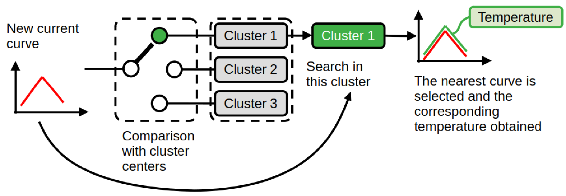A graphical representation is provided by Figure 9. The search for the inductor core temperature using its current curve as a key input can be accomplished by identifying the cluster of the input and then searching in the cluster itself by finding the most similar curve (nearest vector using the Euclidean distance calculated on the samples of the current given by the dataset and experimentally, see Figure 10); this means that the other samples belonging to other clusters are excluded from the search. As it is the similarity query based on a threshold on RMSE, it follows that a search on clusters with superimposed current profiles (such as clusters 0 and 4) will result in several nearest curves complying with the query having different temperature values, resulting in a higher variance or poor accuracy. On the contrary, a cluster in which the curves are different will give a better estimation precision.

The clustering results are obtained using a 10-fold cross-validation technique (the dataset is divided into 10 subsets, and the clustering is repeated 10 times, rotating one subset each time for the test and nine subsets for training, so that all the samples are in the test set once). Using this procedure, and assuming a specific distance range, we considered each curve of the test set as a query for the clustering results and found the nearest current curves in the clustered training set. These current curves are similar to the query curves within the distance range and are members of the same cluster. These retrieved curves are similar to the actual current in the inductor and should reflect its actual operating conditions. In particular, we are interested in the inductor’s temperature, which can be estimated by comparing it to the temperature of the retrieved ones. It is possible to calculate the mean and the standard deviation of the temperature of this set of retrieved curves, and the result is depicted in Figure 11, where it is possible to see that the standard deviation is higher in the clusters number 0 and 4, the two clusters discarded in the considerations before.

6. The Experimental Test Rig

The experimental tests were performed on the LM5122EVM-1PH Evaluation Module (EVM), provided by Texas Instruments Inc. (Dallas, TX, USA), shown in Figure 12. It implements a synchronous DC/DC boost converter using the Texas Instruments LM5122 synchronous boost controller IC. The circuit gives a 24 V output with an input voltage ranging from 9 V to 20 V; the maximum output current is 4.5 A, and the switching frequency is set to 260 kHz. The board is equipped, as standard equipment, with a 10 µH SMD Flat Wire Inductor with linear behavior up to about 9 A, delivered by Würth Elektronik GmbH & Co. KG Circuit Board Technology–Niedernhall-Germany, code 74435561100; however, for the purpose of this paper, the EVM was equipped with the inductor Coilcraft MSS1246-103 exploited as a non-linear inductor. This Coilcraft inductor has the same rated value of 10 µH of the original linear inductor, but its inductance is halved at a lower current, as can be deduced from the manufacturer’s data sheet. Additionally, the manufacturer gives the current values measured with a drop of 10%, 20% and 30% of the rated inductance [44]. The power MOSFETs are N-CH 100 A, 40 V PSMN4R0-40YS by NXP semiconductor, R&D, Milan, Italy. The components are the same as those implemented to build the dataset. The operation mode is set to “forced PWM”; other operations can be set for different purposes, for example, to increase efficiency at light load [45,46].

The measurement system is composed of a power supply GH30-34 from TDK-Lambda (R&D, Milan, Italy), able to vary the supply voltage, and a digital oscilloscope MSO2024B from TEKTRONIX (R&D, Milan, Italy) (with a sample rate of 1 Gs/s) equipped with a current probe TEKTRONIK TCP0020 (20 $A_{rms}$ Maximum Current Capability, and bandwidth from DC to >50 MHz), connected to a terminal of the power inductor to sample its current. A thermal camera FLIR C5, Teledyne (Thousand Oaks, CA, USA) FLIR LLC (±3 °C) provides the inductor temperature. Thermal measurements were conducted using a calibrated thermal camera equipped with analysis tools for defining a rectangular box of interest (Bx1). A fixed box was selected to encompass the expected hotspot region, including the inductor and avoiding other heat sources. For each acquisition, the maximum temperature within Bx1 was recorded and used for validation. It should be noted that the thermal camera captures the surface temperature of the component. While this may raise concerns regarding the internal temperature gradients, in the specific case of the power inductor under test, such gradients are expected to be negligible. This assumption is justified by the small size and low thermal mass of the component, which allows for a rapid thermal equilibrium and limits the formation of internal hotspots. Furthermore, ref. [12] demonstrated in a comparable setup that the surface temperatures show a minimal thermal gradient under steady-state conditions. Based on this, the surface temperature can be considered an adequate approximation of the core temperature for the purpose of validation.

A picture of the inductor is provided in Figure 13; the whole test rig is shown in Figure 14. The EVM board implements the converter described in Section 3. The experimental waveforms of the inductor current are sampled by the oscilloscope allowing comparison with the simulated data.

7. Temperature Estimation

The temperature estimation was carried out on current profiles belonging to different clusters. The comparison is based on the calculation of the root mean square error ($RMSE$), defined as:

$$RMSE(\mathit{x},\mathit{y})=\sqrt{{\displaystyle \frac{1}{N}}\sum _{i=1}^N{(x_i-y_i)}^2}$$

(24)

where $\mathit{x}$ is the simulated inductor current vector, $\mathit{y}$ is the experimental inductor current vector, and N is the number of samples. To assess the accuracy of each profile, the relative root mean square error ($RRMSE$) is employed. It is defined as the ratio between the RMSE and the RMS value of the experimental current:

$$RRMSE(\mathit{x},\mathit{y})={\displaystyle \frac{RMSE(\mathit{x},\mathit{y})}{RMS\left(\mathit{y}\right)}}={\displaystyle \frac{\sqrt{\frac{1}{N}{\sum }_{i=1}^N{(x_i-y_i)}^2}}{\sqrt{\frac{1}{N}{\sum }_{i=1}^N{y}_i^2}}}$$

(25)

The use of the $RRMSE$ allows defining a threshold as a unique adimensional parameter for the whole dataset. The experimental curve is compared with all the simulated profiles within the selected cluster, where clustering is performed based on the current peak value to reduce computational effort.

All simulated current profiles satisfying the condition $RRMSE<threshold$ are kept for further analysis. These M profiles represent plausible candidates that yield sufficiently low error. Since the peak current is particularly sensitive to temperature variations, an additional weighting mechanism is introduced to emphasize this region. For each selected profile, a peak-relative $RMSE$ is computed based only on the current peak:

$$RRMS{E}_{peak}(\mathit{x},\mathit{y})=\sqrt{{\displaystyle \frac{{(\max \left(\mathit{y}\right)-\max \left(\mathit{x}\right))}^2}{\max {\left(\mathit{y}\right)}^2}}}$$

(26)

This value serves as a local sensitivity metric. Its inverse is used to assign a weight to each candidate:

$$w_j={\displaystyle \frac{1}{RRMS{E}_{peak,j}}}$$

(27)

The weights are normalized such that their sum equals one, as follows:

$$w_j^{\prime }={\displaystyle \frac{w_j}{{\sum }_{j=1}^M{w}_j}}$$

(28)

The estimated mean temperature ($\widehat{T}$) is computed as the weighted mean of the M selected temperature values ($T_j$):

$$\widehat{T}=\sum _{j=1}^M{w}_j^{\prime }{T}_j$$

(29)

The associated uncertainty is expressed as a symmetric single $\sigma$ interval as:

$$\sigma =\sqrt{\sum _{j=1}^M{w}_j^{\prime }{(T_j-\widehat{T})}^2}$$

(30)

It is worth noting that clustering reduces the computational effort by limiting the profile comparison to a subset of candidates with similar peak current values.

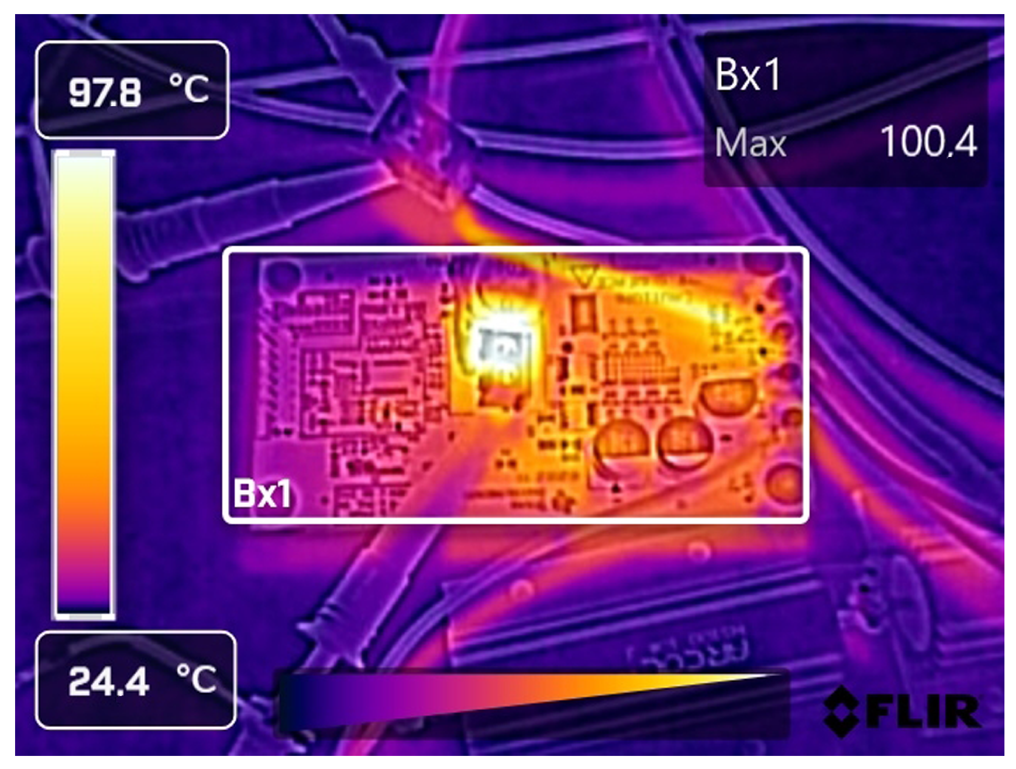
Some characteristic curves were selected for the test; as an example, seven curves are represented in Figure 15 and Figure 16, together with a thermal image, as depicted in Figure 17. The thermal image also shows that the inductor temperature is much higher than the other components of the converter. This operating condition is suitable for converters with inductors operated up to saturation, and justifies the temperature monitoring.

The temperature estimation was carried out firstly by comparing the current waveform spanning the whole dataset. As a final result, the estimated temperature ($\widehat{T}$) with its accuracy was obtained. Furthermore, some other parameters of interest are obtained, such as the estimated input voltage (${\widehat{V}}_{in}$) and the estimated load resistance ($\widehat{R}$). They are provided with the variance ($\sigma$) and coefficient of variation ($CV(\%)=\sigma /\widehat{X}$, where $\widehat{X}$ is the estimated mean value); they are retrieved by the corresponding rows of the dataset belonging to the selected current waveforms. It should be borne in mind that the condition $RRMSE<threshold$ gives several currents, among which, by Equations (29) and (30), the estimation and the uncertainty are calculated. Results were retrieved by assuming a threshold on the $RRMSE=40\%$. To justify the choice of the 40% $RRMSE$ threshold used for filtering candidate current profiles, a sensitivity analysis was performed. The temperature estimation process was repeated for threshold values ranging from 10% to 60% in increments of 10%. As a sensitivity metric, the $CV$ of the estimated temperature was computed for each threshold level. Figure 18 shows the results for the test case at $R=10\mathrm{\Omega }$, depicting the $CV$ as a function of the $RRMSE$ threshold. The analysis reveals that for thresholds above 20%, the $CV$ remains within a narrow range for most temperatures. An exception is observed at 150 °C, where the $CV$ saturates around 40%. Similar results are obtained for the other test cases. This suggests that for $RRMSE$ thresholds larger than 40%, the method becomes relatively insensitive to the threshold, confirming that the estimation is robust and not critically dependent on this parameter.

The results obtained are summarized as the “RMS tolerance method” in

Table 3. Estimation results based on the whole dataset.

RMS tolerance method
Test #	Tcore ( °C)	R ($\mathrm{\Omega }$)	Vin (V)	Current peak (A)	Tolerance (%)	$\widehat{T}$ ( °C)	${\sigma }_T$ ( °C)	$CV$ (%)	${\widehat{V}}_{in}$ (V)	${\sigma }_V$ (V)	$CV$ (%)	$\widehat{R}$ ($\mathrm{\Omega }$)	${\sigma }_R$ ($\mathrm{\Omega }$)	$CV$ (%)
1	50	30	12	2.76	40	107.4	28.5	26.6	13.8	3.0	21.6	26.5	5.8	22.0
2	90	30	12	2.68	40	83.8	36.9	44.1	16.1	2.8	17.5	23.5	5.3	22.4
3	150	30	12	2.68	40	83.8	36.9	44.1	16.1	2.8	17.4	23.5	5.3	22.4
4	30	15	12	4.30	40	87.9	30.4	34.5	13.7	2.0	14.3	14.6	2.7	18.5
5	50	15	12	4.50	40	72.4	34.3	47.4	12.7	3.2	24.9	15.4	4.0	25.9
6	30	10	12	6.36	40	79.1	47.8	60.4	12.8	3.8	29.5	10.9	3.3	30.3
7	50	10	12	6.44	40	67.4	34.3	50.9	13.0	3.1	23.5	9.9	2.5	24.9
8	75	10	12	7.00	40	85.8	42.9	50.0	14.0	3.1	22.2	9.3	2.7	29.0
9	100	10	12	7.80	40	91.2	39.2	42.9	14.2	3.6	25.2	9.0	3.1	34.2
10	120	10	12	9.00	40	78.8	41.0	52.1	14.2	3.1	21.9	7.7	2.8	36.8
11	150	10	12	10.2	40	106.2	35.0	32.9	12.4	2.8	22.7	8.6	2.2	25.8
12	50	15	15	3.68	40	135.8	31.0	22.9	9.9	2.2	22.2	24.5	3.5	14.3
13	90	15	15	3.6	40	82.8	37.2	44.9	13.4	2.7	20.1	19.2	4.1	21.4
14	100	15	15	3.68	40	135.8	31.0	22.9	9.9	2.2	22.2	24.5	3.5	14.3
15	80	10	15	4.96	40	83.5	31.4	37.6	14.4	3.9	27.5	12.4	4.1	32.9
16	100	10	15	5.12	40	75.8	28.0	37.0	12.1	2.5	20.4	13.5	2.5	18.5
17	150	10	15	6.4	40	85.1	38.4	45.1	15.4	3.7	23.7	9.0	3.2	35.6
18	70	20	10	4.08	40	101.4	27.9	27.5	14.5	2.7	18.5	14.6	2.9	19.7
19	100	20	10	6.32	40	80.0	35.0	43.7	13.1	3.4	25.7	10.4	2.9	27.4
20	70	15	10	5.2	40	80.2	37.9	47.2	14.2	3.4	23.7	11.8	3.7	31.1
21	90	15	10	5.2	40	80.2	37.9	47.2	14.2	3.4	23.7	11.8	3.7	31.1
22	100	15	10	5.44	40	88.5	34.2	38.7	12.9	3.5	27.4	12.6	3.6	28.3
23	70	10	10	9	40	78.5	35.1	44.8	14.3	2.7	18.7	7.5	2.2	28.7
24	50	30	9	3.28	40	85.5	31.2	36.4	15.8	4.7	29.8	18.6	7.6	40.6
25	100	15	9	5.52	40	53.3	16.1	30.3	10.5	1.7	16.2	13.7	1.5	10.8
Clustering method
Test #	Tcore ( °C)	R ($\mathrm{\Omega }$)	Vin (V)	Current peak (A)	Cluster #	$\widehat{T}$ ( °C)	${\sigma }_T$ ( °C)	$CV$ (%)	${\widehat{V}}_{in}$ (V)	${\sigma }_V$ (V)	$CV$ (%)	$\widehat{R}$ ($\mathrm{\Omega }$)	${\sigma }_R$ ($\mathrm{\Omega }$)	$CV$ (%)
1	50	30	12	2.76	0	107.1	28.8	26.8	13.8	3.0	21.8	26.4	5.9	22.4
2	90	30	12	2.68	0	84.0	37.0	44.0	16.1	2.9	17.8	23.2	5.4	23.4
3	150	30	12	2.68	0	84.0	37.0	44.0	16.1	2.9	17.8	23.2	5.4	23.4
4	30	15	12	4.30	1	87.9	30.2	34.3	13.7	1.9	13.9	14.3	2.3	15.7
5	50	15	12	4.50	1	71.5	33.9	47.4	12.7	3.2	25.0	15.1	3.7	24.8
6	30	10	12	6.36	1& 2	79.4	47.4	59.8	12.8	3.8	29.3	11.1	3.5	31.5
7	50	10	12	6.44	1&2	68.0	34.5	50.7	13.0	3.1	23.5	10.1	2.8	28.0
8	75	10	12	7.00	1&2	85.9	42.5	49.5	14.0	3.1	22.4	9.7	3.3	34.0
9	100	10	12	7.80	2	92.7	39.7	42.8	14.4	3.6	25.2	8.3	2.5	34.2
10	120	10	12	9.00	2	78.4	41.8	53.4	14.3	3.2	22.0	7.4	2.4	32.7
11	150	10	12	10.2	2&3	102.2	37.0	36.2	13.1	3.4	25.8	7.8	2.2	28.3
12	50	15	15	3.68	0	135.7	31.1	22.9	10.0	2.3	23.0	24.6	3.4	13.8
13	90	15	15	3.6	0	82.8	37.2	44.9	13.6	2.8	20.3	19.7	4.3	21.7
14	100	15	15	3.68	0	135.7	31.1	22.9	10.0	2.3	23.0	24.6	3.4	13.8
15	80	10	15	4.96	1	83.3	31.2	37.4	14.4	4.0	27.5	12.2	3.9	32.2
16	100	10	15	5.12	1	75.5	27.7	36.8	12.1	2.4	20.1	13.5	2.4	17.6
17	150	10	15	6.4	1&2	84.9	38.4	45.3	15.4	3.7	23.9	8.9	3.1	34.9
18	70	20	10	4.08	0&1	101.2	28.1	27.7	14.5	2.7	18.5	14.7	3.1	20.9
19	100	20	10	6.32	1&2	80.1	35.1	43.8	13.1	3.4	25.7	10.5	3.0	28.3
20	70	15	10	5.2	1	80.0	37.9	47.4	14.2	3.4	23.7	11.7	3.6	30.6
21	90	15	10	5.2	1	80.0	37.9	47.4	14.2	3.4	23.7	11.7	3.6	30.6
22	100	15	10	5.44	1	88.3	34.2	38.8	12.9	3.5	27.4	12.6	3.5	28.1
23	70	10	10	9	2	78.4	35.1	44.8	14.3	2.6	18.4	7.4	2.0	27.4
24	50	30	9	3.28	0	85.5	31.3	36.6	15.8	4.7	29.5	18.7	7.6	40.4
25	100	15	9	5.52	1	53.2	16.0	30.1	10.5	1.7	16.2	13.7	1.5	10.8

, where the experimental values are compared with the estimated ones. Secondly, the same estimation is performed by exploiting the clustering features. This means that, instead of the whole dataset, the spanning covers only the cluster to which the current waveform (identified by its maximum) belongs. The results are identified in Table 3 by “Clustering method”. To evaluate the robustness of the temperature estimation approach, the method was tested across a variety of operating conditions. The experimental setup was configured to operate the boost converter with input voltages of 9 V, 10 V, 12 V, and 15 V, and load resistances of 10 $\mathrm{\Omega }$, 15 $\mathrm{\Omega }$, 20 $\mathrm{\Omega }$, and 30 $\mathrm{\Omega }$. The converter is equipped with a regulation loop that maintains a fixed output voltage of 24 V by automatically adjusting the duty cycle of the switching signal based on the input voltage value. These test cases span a range of input voltage and power levels, resulting in different current waveforms.

The measured temperature values used for validation are acquired through the thermal camera with an accuracy of ±3 °C; each obtained value defines the reference temperature in our evaluation. The estimation process, however, does not involve any direct temperature measurement and is entirely based on simulation and profile matching. The uncertainty of the estimated temperature is obtained by computing the weighted standard deviation over the accepted candidate temperatures. The weights reflect the relative matching quality, and the resulting spread provides an indication of the internal confidence of the estimation process. This approach does not explicitly include uncertainty from the simulation model, which is not trivial to assess. However, the scope of this paper is to determine whether the method yields a reliable estimate that falls within the accuracy range of the thermal camera. In all tested conditions, the estimated temperature lies within this range, supporting the robustness of the proposed estimation strategy. Similar consideration can be extended for the waveforms acquisition equipment, i.e., oscilloscope and current probe, which introduce a modest measurement error.

Concerning results obtained by spanning the whole dataset in the “RMS tolerance method”, as expected, the estimation in the linear operating region of the inductor, where the current waveforms are superimposed, as depicted in Figure 7a, gives a poor accuracy, resulting in high error between the real value and the estimated one and a high coefficient of variation. The same situation occurs for high temperature and high currents, corresponding to Figure 7c. On the contrary, the estimation performed on currents as described by Figure 7b gives better values.

The results obtained by the clustering method are similar; however, they are obtained by searching within a reduced dataset defined by the clusters. When a current waveform belongs to two contiguous clusters they are both considered (as an example, the notation “1&2” means that clusters 1 and 2 are taken into account). A graphical representation of the results is provided by Figure 19 for the experiments identified as $Test6$, $Test8$, $Test9$, $Test11$, $Test17$, $Test19$, and $Test25$ conducted at $T_{core}$, ranging from 30 to 150 °C (Figure 19a), $V_{in}$, ranging from 9 to 15 V (Figure 19b), and with R from 10 to 20 $\mathrm{\Omega }$ (Figure 19c). Low and very high temperature ($Test6,Test9$ and, $Test11$ of Figure 19a) are poorly estimated; however, they do not have a practical interest. Instead, for $Test8,Test9,$ and $Test19$, the real value is near the estimated one and the $\sigma$ interval always contains the real value. The last diagram represents a test case within cluster 0 and the temperature is underestimated. With reference to voltage and load resistance estimation, the real estimated value approaches the real one within one $\sigma$ interval; instead, for the case with high resistance ($Test25$ at 20 $\mathrm{\Omega }$), the resistance is underestimated. To visually represent the dispersion and reliability of the temperature estimation across different test cases, weighted boxplots were constructed based on the empirical distribution of temperatures for the $Test6$, $Test8$, $Test9$, $Test11$, $Test17$, $Test19$, and $Test25$ in Figure 20. The box spans from the 25th to the 75th percentile, capturing the interquartile range (IQR) in the same way as the coefficient of variation, while the whiskers extend from the 5th to the 95th percentile. This representation avoids assumptions of normality and provides a robust description of the central tendency and spread. The median temperature (50th percentile) is shown as a thick black line, while the weighted mean is overlaid as a red circle to highlight its role as the main estimator used throughout the study. Values falling outside the 5th–95th percentile range are shown as crosses and represent potential outliers. In $Test25$, the boxplot displays an unusually narrow interquartile range with a high concentration of outliers. This behavior is caused by the specific weighted distribution used for this estimation. Specifically, the cumulative sum of the normalized weights reveals a sharp transition from 0.05 to 0.91 between two consecutive temperature values, indicating that approximately 86% of the total weight is concentrated in a single candidate. This means that the estimation process heavily favored one particular current profile due to its exceptionally low peak error, while all other profiles, despite being within the same cluster, received negligible weights and appear as statistical outliers in the boxplot. Interestingly, this dominant solution does not coincide with the reference value measured by the thermal camera, highlighting a potential sensitivity of the weighting mechanism to local minima in the error residuals.

Finally, the main advantages in terms of computational saving are summarized in

Table 4. Computational effort reduction.

Cluster Number	Number of Samples in Cluster	Computational Effort Reduction
0	2477	43%
1	1005	77%
2	419	90%
3	330	92%
4	137	97%

. The estimation for temperature belonging to clusters 2 and 3 shows a computational effort reduction of 88% and 90%, respectively.

8. Discussion and Method’s Generalization

Although the adopted dataset is relatively small, by varying other parameters, such as the input voltage or converter output capacitance, it can become much larger in size, justifying the need to reduce the computational effort. In perspective, modern switching converters will adopt higher switching frequencies, posing an upper limit on the computational time. In fact, in most applications, the elaboration must be performed in a time interval defined by the inverse of the switching frequency. Finally, power density and cost design constraints require embedded low-cost hardware. The proposed estimation method requires accurate acquisition of the inductor current waveform within a switching period. In the experimental setup, the converter operates at a switching frequency of 260 kHz, and a sampling resolution of 20 points per cycle is adopted. This implies a minimum required bandwidth of 5.2 MHz for the acquisition system. Thermal variations, however, occur over significantly longer timescales (tens to hundreds of seconds), due to the thermal inertia of the components. Therefore, the estimation process can be performed asynchronously and averaged over multiple switching cycles, mitigating the impact of high-frequency noise. In the laboratory, inductor current measurements were obtained using a 50 MHz bandwidth current probe connected to a digital oscilloscope. For embedded implementations, a Hall-effect current sensor interfaced with a microcontroller is a viable alternative. Such sensors typically exhibit 1–2% full-scale accuracy and bandwidths that are sufficient to capture the relevant features of the current waveform necessary for temperature estimation.

The proposed method can be generalized to applications in which a similarity comparison among many time-series, with a characteristic parameter, is required; although many classification methods based on neural networks exist, the K-means clustering, being based on characteristic parameters, is explainable, meaning that the decision is transparent and understandable to humans.

9. Conclusions

The temperature of an inductor magnetic core, operated in a switching converter, can be retrieved based on its current profile. The proposed method allows estimating the steady-state temperature for given operating conditions, allowing forecasting of dangerous working conditions. The estimation is carried out by comparison with a dataset obtained by simulation. The K-means clustering applied to current waveforms, with their maximum value as parameters, allowed identification of the regions in which the estimation can be retrieved with better accuracy and reduction in the computational effort by up to 90% in the region of interest.

The proposed method can be applied to a large dataset to reduce computation time and foster implementation in low-cost hardware platforms.