Article

A Novel FMCW LiDAR Multi-Target Denoising Method Based on Optimized CEEMDAN with Singular Value Decomposition

1
School of Microelectronics, Tianjin University, Tianjin 300072, China
2
Tianjin Key Laboratory of Imaging and Sensing Microelectronic Technology, Tianjin 300072, China
*
Authors to whom correspondence should be addressed.
Electronics 2025, 14(13), 2697; https://doi.org/10.3390/electronics14132697
Submission received: 5 May 2025 / Revised: 30 June 2025 / Accepted: 1 July 2025 / Published: 3 July 2025
(This article belongs to the Section Circuit and Signal Processing)

Abstract

Frequency-modulated continuous-wave (FMCW) LiDAR systems frequently experience noise interference during multi-target measurements in real-world applications, resulting in target overlapping and diminished detection accuracy. Conventional denoising approaches—such as Empirical Mode Decomposition (EMD) and wavelet thresholding—are often constrained by challenges like mode mixing and the attenuation of weak target signals, which limits their detection precision. To address these limitations, this study presents a novel denoising framework that integrates an optimized Complete Ensemble Empirical Mode Decomposition with Adaptive Noise (CEEMDAN) algorithm and singular value decomposition (SVD). The CEEMDAN algorithm’s two critical parameters—the noise standard deviation and the number of noise additions—are optimally determined using particle swarm optimization (PSO), with the envelope entropy of the intrinsic mode functions (IMFs) serving as the fitness criterion. IMFs are subsequently selected based on spectral and amplitude comparisons with the original signal to facilitate initial signal reconstruction. Following CEEMDAN-based decomposition, SVD is employed with a normalized soft thresholding technique to further suppress residual noise. Validation using both synthetic and experimental datasets demonstrates the superior performance of the proposed approach over existing methods in multi-target scenarios. Specifically, it reduces the root mean square error (RMSE) by 45% to 59% and the mean square error (MSE) by 34% to 69%, and improves the signal-to-noise ratio (SNR) by 1.85–4.38 dB and the peak signal-to-noise ratio (PSNR) by 1.18–6.94 dB. These results affirm the method’s effectiveness in enhancing signal quality and target distinction in noisy FMCW LiDAR measurements.

1. Introduction

Frequency-modulated continuous-wave (FMCW) LiDAR is a promising sensing technology that integrates LiDAR with FMCW radar principles, combining optical, mechanical, and electronic components to enable high-resolution distance and velocity measurements [1]. It has gained widespread application in fields such as autonomous driving and atmospheric monitoring due to its robustness and precision [2,3]. However, in complex and dynamic environments, FMCW LiDAR signals are often subject to various sources of interference during transmission and reception. These include photodetector dark currents, thermal noise from electronic circuits, and ambient stray light, particularly solar radiation [4,5,6]. In scenarios involving multi-target detection at close range, such interference becomes more pronounced, often leading to signal aliasing, degradation of weak targets, and reduced recognition accuracy due to low signal-to-noise ratios (SNRs).
To mitigate noise and improve target recognition, a variety of denoising techniques have been employed. Classical methods such as the Fourier transform and Savitzky–Golay filtering are effective for stationary or linear signals but tend to underperform with nonlinear and nonstationary data [7,8,9,10]. Empirical Mode Decomposition (EMD) [11,12,13], a fully data-driven technique, is better suited for such signals, offering adaptive decomposition without requiring a priori basis functions [14,15]. However, EMD suffers from mode mixing and poor frequency resolution, which limits its reliability in practical applications [16,17,18].
To address these shortcomings, Ensemble Empirical Mode Decomposition (EEMD) was proposed, introducing white noise to the original signal and averaging multiple decompositions to suppress mode mixing [19,20,21]. While EEMD improves decomposition stability, it also introduces new issues in denoising applications—particularly for FMCW LiDAR—where the frequency content varies with target distance. As a result, useful signal components may be spread across multiple intrinsic mode functions, complicating their isolation and reconstruction.
Building on EEMD, the Complete Ensemble Empirical Mode Decomposition with Adaptive Noise (CEEMDAN) algorithm was developed to further enhance decomposition accuracy and reduce reconstruction error [22]. Unlike EEMD, CEEMDAN progressively adds adaptive white noise and computes IMFs by decomposing the residual at each stage. This results in improved mode separation and reduced interference between components. Nevertheless, CEEMDAN’s effectiveness is highly sensitive to the selection of key parameters, particularly the standard deviation of added noise and the number of noise realizations. Inappropriate parameter settings can lead to either insufficient decomposition or the inclusion of residual noise, highlighting the need for robust and automated parameter optimization.
To address this challenge, this paper proposes a novel denoising method that combines CEEMDAN with particle swarm optimization (PSO) [23] and singular value decomposition (SVD) [24,25] to improve multi-object detection performance in FMCW LiDAR. The PSO algorithm is employed to optimize the noise-related parameters of CEEMDAN, using the envelope spectral entropy as the fitness function to ensure optimal IMF separation. After decomposition, windowed FFT is applied to the IMFs to obtain frequency and amplitude spectrum information. Based on the system’s spatial resolution and the amplitude of the target signals, useful IMFs are identified and filtered, followed by further SVD processing. By normalizing and soft thresholding the singular values, the most significant signal components are retained while significantly reducing noise components. Finally, low-rank signal reconstruction is performed to obtain the final signal denoising results. Experimental results demonstrate that this approach achieves superior noise suppression and signal fidelity in both synthetic and real-world multi-target scenarios.
In summary, the principal contributions of this paper are outlined as follows:
(1)
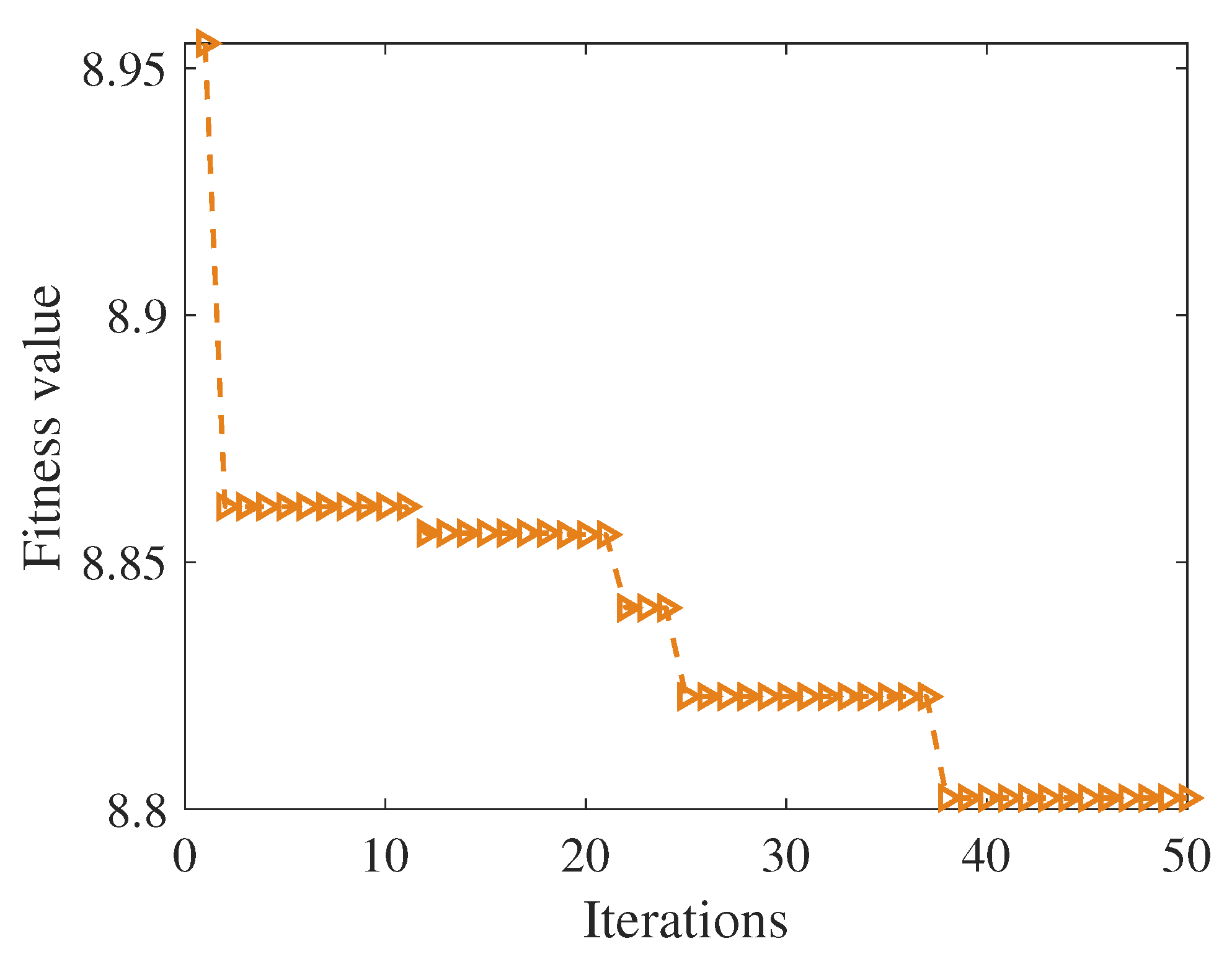
Integration of the particle swarm optimization (PSO) algorithm optimizes the noise addition frequency and standard deviation parameters in the CEEMDAN method. This optimization enhances decomposition, minimizes mode mixing, and ensures modal functions do not carry excess interference or lose valuable information. Envelope entropy serves as the optimization fitness function, refining the CEEMDAN algorithm’s effectiveness.
(2)
For the IMFs generated by the CEEMDAN algorithm, this study proposes a method that performs windowed FFT operations on the original signal and the CEEMDAN-processed IMFs, and then uses a comparison algorithm that combines frequency and amplitude spectra to determine the IMFs containing useful signals and filter out other IMFs that are mainly noise.
(3)
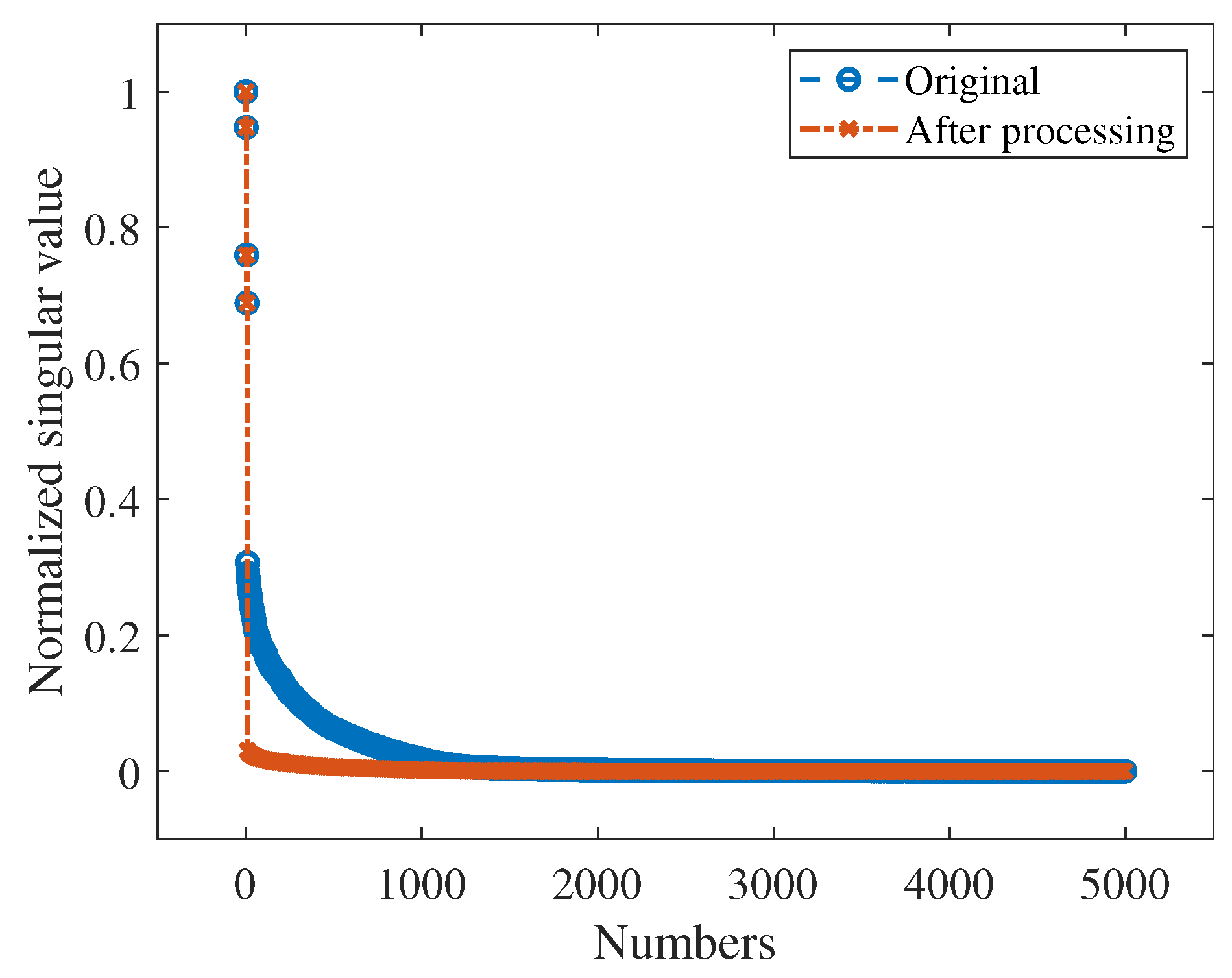
The SVD algorithm is used to further decompose the retained IMF components. The value with the largest change in the singular value difference is used as the basis for determining the reconstruction order, so as to achieve a low-rank singular value matrix and thereby achieve efficient signal denoising.
The remainder of this article is organized as follows: Section 2 explicates the principles of the proposed denoising method; Section 3 validates its effectiveness through simulations and experimental data, comparing it to documented methods to demonstrate its superior performance; and Section 4 concludes the paper.

2. Methodology

For FMCW LiDAR, the IF signal can be expressed by (1):
f I F = 4 × R × B c × T
where c represents the speed of light, approximately 3 × 10 8 m / s , T is time range of the triangular wave sweeping periods, R is the object’s distance, and B is the modulation bandwidth. The signal after ADC (Analog-to-Digital Converter) sampling and the FFT (Fast Fourier Transform) is as follows:
X k = w ( n ) n = 0 N 1 x n e j 2 π k n / N
Here, we use the Hanning window function w ( n ) to effectively reduce spectrum leakage and side lobe interference. After a peak search in the frequency spectrum to determine the frequency of the target corresponding to the location X j ( 1 j k ) , when several targets’ echo is reflected back, there will be more than one target component in the signal spectrum X j 1 , X j 2 , X j 3 , ( 1 j 1 , j 2 , j 3 , k ) . Due to the impact of the target distance and reflectivity, the echo signal frequency and amplitude are not the same, and both of them directly reflect the target distance and intensity of the feature information; therefore, the denoising algorithm needs to try to ensure the characteristics of the echo signal and, at the same time, remove the excess noise in the frequency band.

2.1. CEEMDAN Method

The CEEMDAN method introduces several notable advancements over the conventional EEMD (Ensemble Empirical Mode Decomposition) algorithm. One key enhancement in CEEMDAN is the adaptive introduction of white noise at each stage of the signal decomposition process, which is followed by the computation of a unique residual for each iteration. This iterative incorporation of noise facilitates the superposition and eventual cancellation of noise components across multiple iterations. Through this process, reconstruction errors are progressively minimized at each stage, allowing for significantly improved accuracy in the decomposition of complex signals. As a result of this iterative noise-cancellation mechanism, CEEMDAN achieves an almost negligible reconstruction error for each decomposed IMF. This refinement ensures that CEEMDAN is highly effective in separating individual signal components, thereby providing a more robust solution for analyzing and processing.
x ( t ) is the original signal and a Gaussian white noise sequence with standard normal distribution is added to x ( t ) for the ith time to obtain x i ( t ) :
x i ( t ) = x ( t ) + ε 0 ω i ( t ) , ( i = 1 , 2 , 3 , , I )
where ε 0 is the noise factor and ω i is the ith Gaussian white noise with N ( 0 , σ 2 ) . The SNR is adjusted at each stage of the signal differently so as to achieve the process of adaptive decomposition. E k ( · ) is denoted as the kth IMF decomposed by the EMD algorithm, and the first IMF obtained by CEEMDAN for the signal is denoted as follows:
i m f ˜ 1 ( t ) = 1 I i = 1 I i m f 1 i ( t ) , ( i = 1 , 2 , 3 , , I )
Then, the residue r 1 ( t ) of the first IMF i m f ˜ 1 ( t ) is as follows:
r 1 ( t ) = x ( t ) i m f ˜ 1 ( t )
We can obtain I group signals r 1 ( t ) + ε 1 E 1 ( ω i ( t ) ) ( i = 1 , 2 , 3 , , I ) and decompose these signals using the EMD algorithm, and then the second-order IMF i m f 2 ˜ ( t ) can be expressed as follows:
i m f 2 ˜ ( t ) = 1 I i = 1 I E 1 ( r 1 ( t ) + ε 1 E 1 ( ω i ( t ) ) )
For the remaining j = 2 , 3 , 4 , , J , (4)–(6) are repeated, and the jth residue r j ( t ) is defined as follows:
r j ( t ) = r j 1 ( t ) i m f ˜ j ( t )
EMD is performed on the Gaussian white noise ω i ( t ) to obtain the adaptive noise, the decomposed adaptive noise is added to the residual, and the new signal to be separated is obtained as follows:
x i ( t ) = r j 1 ( t ) + ε j 1 E j 1 ( ω i ( t ) )
where ε j 1 represents the added noise amplitude when solving for the jth IMF i m f ˜ j ( t ) , and operations (3) and (4) are performed on x i ( t ) . Then, we can obtain i m f ˜ j ( t ) as follows:
i m f ˜ j ( t ) = 1 I i = 1 I E 1 ( r j 1 ( t ) + ε j 1 E j ( ω i 1 ( t ) ) )
The jth residue can be represented as follows:
r j ( t ) = r j 1 ( t ) i m f ˜ j ( t )
Therefore, the original signal x ( t ) can be expressed as follows:
x ( t ) = j = 1 J i m f ˜ j ( t ) + r j ( t )
After obtaining i m f ˜ j ( t ) using the CEEMDAN algorithm, each IMF needs to be screened. We choose IMF automatic screening based on spectral analysis. First, FFT is performed on the original signal x ( t ) to obtain the amplitude spectrum | X ( f ) | , and N significant peaks { f 1 , f 2 , f 3 , } from the amplitude spectrum. For each target frequency f k , we set a bandwidth range Δ f . Here, the bandwidth range of the signal is determined by the maximum spatial resolution of the FMCW LiDAR, which is c / 2 B [26]. Substituting into Equation (1), we obtain Δ f = 2 / T . Therefore, the target frequency neighborhood is defined as follows:
f k m i n = f k Δ f f k m a x = f k + Δ f
Then, IMF selection is performed, and FFT is performed on each i m f ˜ j ( t ) to obtain its amplitude spectrum | I M F ˜ j ( f ) | . Then, the target peaks in the IMF spectrum are detected to see if there are significant peaks in the target frequency neighborhood [ f k min , f k max ] . If there are peaks, (13) is used to finally determine whether the IMF contains the target signal component and decide whether to keep it or discard it, where we can set α = 0.3 .
| I M F j ˜ ( f k ) | > α · max ( | I M F j ˜ ( f ) | )
Then, the new processed original signal x ˜ ( t ) after IMF selection can be expressed as follows:
x ˜ ( t ) = j = k i m f ˜ j ( t ) + r j ( t )
However, the choice of white noise addition amount i and noise standard deviation σ has an important influence on obtaining the best SNR for the main IMF signal. Therefore, we choose the PSO algorithm to optimize these parameters.

2.2. CEEMDAN Parameters Optimized by PSO Method

While the CEEMDAN algorithm successfully mitigates the issues of modal aliasing and endpoint effects inherent in the EMD algorithm, the method still requires an optimization process to determine two critical parameters: the number of white noise realizations, denoted as i, and the noise standard deviation, ε . These parameters are not predefined, and their selection significantly impacts the effectiveness of the CEEMDAN. Typically, the values for these parameters are determined based on empirical knowledge, lacking formalized or rigorous justification, which can introduce variability and uncertainty in the results.
In the CEEMDAN algorithm, the optimization of the parameters i and σ constitutes a low-dimensional optimization problem, rendering the computational cost particularly sensitive. Given that each CEEMDAN requires repeated noise additions and iterative extraction of intrinsic mode functions (IMFs), an optimization method with rapid convergence is essential. In this study, the particle swarm optimization (PSO) algorithm is employed to optimize these two parameters. Compared to alternative approaches such as Genetic Algorithms (GA) and Bayesian Optimization (BO), PSO demonstrates superior convergence efficiency in low-dimensional settings. This advantage can be attributed to its mechanism of velocity and position updates, which enables efficient exploration and exploitation of the search space. In contrast, GA involve computationally intensive operations including crossover, mutation, and selection, while BO requires the construction and updating of surrogate models. Consequently, PSO offers a more streamlined and computationally efficient optimization process particularly suitable for problems involving a limited number of parameters [27]. Additionally, PSO’s swarm intelligence characteristics make it robust to initial parameter distributions, enabling efficient exploration of global optima across a wider parameter range. Meanwhile, GA’s crossover and mutation operations are inefficient in low-dimensional problems and require extensive population iterations, leading to high computational costs and potential local optima traps. BO performs excellently in high-dimensional problems but faces issues such as high computational overhead and strong prior dependencies in low-dimensional parameter optimization tasks.
The PSO algorithm primarily adjusts the adaptability of particles to the environment through particle state initialization, continuous optimization search, and iterative comparison of the optimal solution of individuals with the global optimal solution, thereby searching for the optimal solution within the target region. The PSO algorithm can be described in detail as follows: In a D-dimensional space, there is a population X consisting of m particles. The ith particle moves at velocity V i = ( v i 1 , v i 2 , , v i D ) , the position of each particle in space is denoted as X i = ( x i 1 , x i 2 , , x i D ) , the optimal position of each particle is denoted as P i = ( p i 1 , p i 2 , , p i d ) , and the optimal position of the population is P g = ( p g 1 , p g 2 , , p g d ) . The k + 1 th dimension velocity v i d k + 1 and x i d k + 1 can be expressed as follows:
v i d k + 1 = w v i d k + c 1 η ( p i d x i d k ) + c 2 η ( p g d x i d k ) x i d k + 1 = x i d k + v i d k + 1
where 1 i m , 1 d D , k is the number of current iterations, c 1 and c 2 are learning factors, w is the inertia weight, and η is a random number within 0 , 1 .
The envelope spectral entropy value of a signal [28] reflects its randomness and complexity. The more periodic the signal, the lower its complexity and the smaller the entropy value. Conversely, the more non-periodic noise interference there is, the more complex the signal and the larger the entropy value. Therefore, this paper adopts the envelope spectrum entropy as the fitness function for the PSO algorithm. The envelope spectrum entropy of the IMF components obtained after decomposing the original signal using the CEEMDAN algorithm can be expressed as follows:
E i = j = 1 N p i , j lg p i , j p i , j = a i ( j ) / j = 1 N a i ( j )
where i represents the index of IMF components derived from the CEEMDAN of the original signal. The envelope spectrum of the i-th IMF, denoted as a i ( j ) , is obtained through the application of the Hilbert transform, and its normalized form is expressed as p i , j . When CEEMDAN successfully isolates IMFs with well-defined laser intermediate-frequency components, the associated envelope spectrum entropy assumes relatively low values, reflecting the presence of strong periodic structures. In contrast, a higher entropy value indicates a reduced presence or increased irregularity of periodic components within the IMFs. Accordingly, the envelope spectrum entropy serves as the objective function in the PSO algorithm, guiding the optimization process toward enhanced identification of IF signals with pronounced periodic characteristics.
The PSO-CEEMDAN algorithm determines the search process for two parameters as follows:
Step 1: The parameters of the PSO are initialized and the minimum value of the envelope entropy E i is used as the fitness function of the particle swarm algorithm.
Step 2: Particle positions ( k , σ ) and particle velocities v i d are randomly generated in the particle population.
Step 3: CEEMDAN calculates the E i value corresponding to each particle position for the signal at different particle positions ( k , σ ) .
Step 4: Individual extremes and population global extremes are updated by constantly comparing the size of E i .
Step 5: The particle travel speed and position are updated using (12) and (13).
Step 6: Steps 3∼5 are looped, and when the number of iterations reaches the preset maximum value, the loop ends and outputs the best particle position ( k , σ ) .

2.3. IMF Decomposition by SVD Method

After optimizing the parameters of CEEMDAN using the PSO algorithm and decomposing it to obtain the preliminary denoised signal x ˜ ( t ) , although the useful signal is more concentrated, there is still a large amount of residual noise. In this paper, we choose the singular value decomposition method to further denoise x ˜ ( t ) , and then reconstruct it to obtain the final denoised result. First, the input signal x ˜ = [ x ˜ ( 1 ) , x ˜ ( 2 ) , , x ˜ ( N ) ] is transformed into a Hankel matrix as follows:
H = x ˜ ( 1 ) x ˜ ( 2 ) . . . x ˜ ( n ) x ˜ ( 2 ) x ˜ ( 3 ) . . . x ˜ ( n + 1 ) x ˜ ( m ) x ˜ ( m + 1 ) . . . x ˜ ( n + m 1 )
Here, N = m + n 1 , and the Hankel matrix H is composed of a set of row vectors, where each subsequent row vector lags behind the previous row vector by one data point. When this matrix is constructed using ideal noise-free signals, it becomes a singular matrix, exhibiting high correlation between adjacent row vectors. In such matrices, the initial singular values are large but rapidly decay to near zero, with the decay threshold being related to the matrix rank, indicating a significant transition phenomenon in the singular values. In contrast, Hankel matrices constructed from noisy data exhibit similar delays between row vectors but lack such correlations, thereby maintaining a full rank. Therefore, accurately characterizing the singular value fluctuations caused by noise signals is a core challenge when applying singular value decomposition for denoising. According to singular value decomposition theory, for a matrix H of dimension m × n and rank r, the decomposition form is as follows:
H = U Σ 0 0 0 V T
where U and V are unitary matrices of dimensions m × m and n × n , respectively, Σ is an r-dimensional diagonal matrix whose diagonal elements are the nonzero singular values ξ i ( i = 1 , 2 , , r ) of the matrix H, and the sequence formed by all the singular values in descending order is S = ξ 1 ξ 2 ξ r , where r = min ( m , n ) .
The singular values represent the energy contained in each component of the signal. Larger singular values typically correspond to important components of the signal, while smaller values indicate noise components. When the signal strength is much greater than the noise strength and the noise source is singular, a hard threshold method can be used to retain only the largest k singular values in the diagonal matrix and set all values below k to zero. Common methods include those based on the singular value difference spectrum [25]. The threshold k is typically chosen based on the point of maximum variation in the singular values, which marks the boundary between the signal and noise. However, in multi-target FMCW LiDAR systems, due to high noise intensity and complex noise sources, traditional hard thresholding methods may fail to effectively distinguish between signals and noise. In such cases, normalized soft thresholding methods are more effective. This method normalizes singular values by calculating the ratio of each singular value to the maximum singular value, thereby quantifying the amount of useful information carried by each value while preserving the distribution pattern of singular values. Normalization is used to determine an appropriate denoising level, and the effective denoising order k is determined based on the normalized singular value intensity μ .
ξ i ¯ = ξ i ξ 1 ( i = 1 , 2 , , r )
μ = 0.5 and the largest integer k are taken such that ξ ¯ k μ is found. The singular values greater than k represent the singular value portion where the main signal energy is concentrated, while those less than k represent the singular value portion where weak signal energy and main noise are concentrated. Here, unlike in the hard threshold method, singular values of less than k are no longer directly set to 0, but are instead divided by a coefficient β . The value of β is set to the value corresponding to the kth original singular value, as shown in Equation (19).
ξ i i = 1 , 2 , , k 1 ξ i / β others
If the threshold β = 0 , it degenerates into hard threshold singular value denoising. This method can maximize the retention of useful signal components, making the denoising results smoother and better preserving signal continuity compared to the abrupt truncation of hard thresholds. The signal is then reconstructed according to the new singular value sequence ξ i as follows:
H = i = 1 r u i ξ i v i T
where u i , v i are the ith vector of U and V . Then, the reconstructed signal x ¯ obtained by the SVD algorithm can be expressed as follows:
x ¯ = H 1 , p H m , q n + 1 , ( p = 1 , 2 , , n ; q = n , n + 1 , , 2 n 1 )
As depicted in Figure 1, the algorithm presented herein initiates by conducting an FFT on the noisy IF signal to identify the frequency associated with the maximal spectral peak. Subsequent to this, the CEEMDAN algorithm is applied to the noisy IF signal. Concurrently, the particle swarm optimization algorithm is employed to refine the input parameters for the CEEMDAN, specifically the number of noise additions i and the standard deviation of the noise σ . The optimization targets the minimization of the envelope entropy of the ultimately decomposed noise signal, which serves as the fitness function guiding the cessation of optimization. Following this, additional IMFs are extracted via FFT and peak detection techniques. These IMFs are either retained or discarded based on a comparison with predetermined parameters. The next phase involves the application of the SVD technique on the preserved IMFs, whereby larger singular values associated with predominant signal components are retained as by (18). The singular values ξ , predominantly affiliated with noise components and fewer signal components, are reduced via a coefficient β , facilitating soft thresholding denoising. Ultimately, the refined singular values are utilized to reconstruct the denoised signal as delineated in (19)–(21), completing the signal-processing workflow.

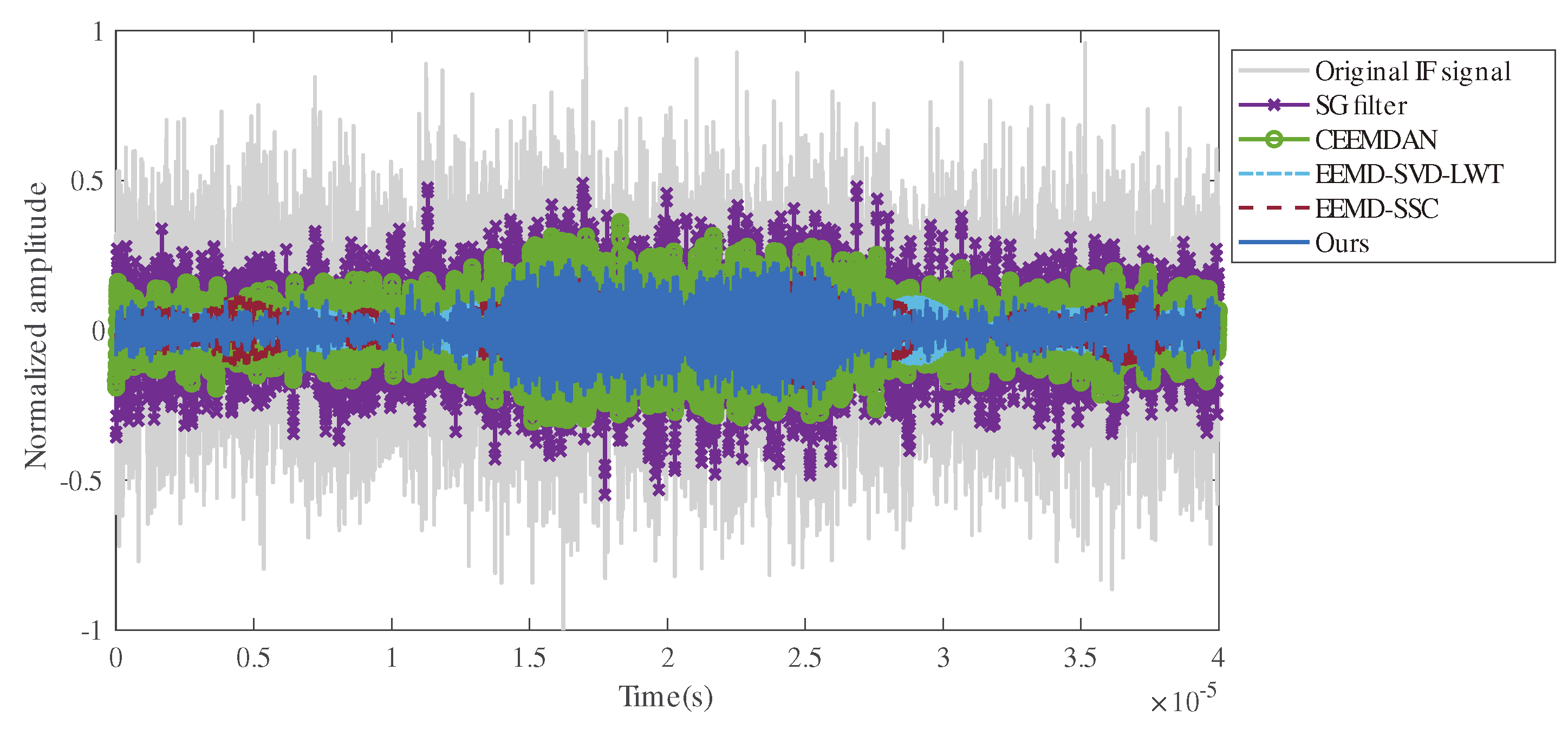
3. Performance Evaluation

In this chapter, the efficacy and performance of the proposed algorithm are validated using both simulated and real signal data.

3.1. Synthetic Signal Evaluation

In this study, the synthetic signal superimposed with Gaussian white noise was used as the simulation signal to verify the effectiveness of the proposed method in MATLAB v2021a (MathWorks Inc. (Natick, MA, USA)) on a Lenovo R9000P laptop (AMD (Santa Clara, CA, USA) Ryzen7 5800H, 32GB memory). Two numerical experiments were used to verify the validity and superiority of our proposed method with the following simulation parameters: a sampling period of 5 μs, a number of samples of 10,000, a sampling rate of 200 MHz, and a signal bandwidth of 100 MHz.
Based on the FMCW LiDAR realistic multi-target scenario, it is known from (1) that different targets correspond to different frequency values; therefore, we synthesized the echo signals of multiple targets, and the setting parameters were as shown in Table 1.
f ( t ) = A 1 sin ( 2 π f 1 t + φ 1 ) + A 2 sin ( 2 π f 2 t + φ 2 ) + A 3 sin ( 2 π f 3 t + φ 3 ) + A 4 sin ( 2 π f 4 t + φ 4 )
We set a Gaussian white noise of −8 dB, −6 dB, −4 dB, and −2 dB separately, and the sampling rate was 100 MHz, the number of sampling points 5000, and the sampling period 50 μs. The synthetic signals are shown in Figure 2.
Subsequently, the parameters of the CEEMDAN method were optimized through the application of the PSO algorithm. Specifically, this optimization targets two key parameters: the number of noise realizations and the noise standard deviation. The permissible range for the number of noise additions was defined within the interval of [0.01, 0.4], while the noise standard deviation was constrained within [10, 400]. Other parameter settings were as shown in Table 2.
This process of optimization is critical for balancing the trade-off between noise suppression and signal preservation within the CEEMDAN framework. By employing the PSO algorithm, optimal or near-optimal parameter values that minimize noise interference while retaining the essential features of the original signal are efficiently located. The iterative nature of the PSO allows for progressively improved solutions, which are tracked and evaluated over the course of multiple runs. The results of this optimization process are visually depicted in Figure 3. The figure illustrates how variations in iteration count and parameter settings influence the performance of the CEEMDAN algorithm, providing insights into the trade-offs involved in selecting the optimal balance between noise addition and standard deviation for different noise environments. Through this comprehensive evaluation, the PSO-enhanced CEEMDAN approach demonstrated improved adaptability and robustness in handling complex signal denoising tasks.
After 50 iterations, the fitness value reached 8.8, with a corresponding noise addition amount i of 67 and a noise standard deviation σ of 0.09. Subsequently, we ran the CEEMDAN algorithm again and obtained multiple IMF components and a residual through Equations (4) and (5). We then selected the useful IMF components from the decomposed results using Equations (12) and (13), reconstructed the selected IMF components, and applied the SVD algorithm according to Equations (17) and (18). From the diagonal elements of the resulting singular value matrix Σ , we obtained the singular value sequence S. We then applied the soft threshold normalization method shown in (19) and (20) to process the singular value sequence, obtaining a new singular value sequence, as shown in Figure 4. Finally, we obtained the new reconstructed denoised signal using (21) and (22).
The Savitzky–Golay filtering algorithm [8], CEEMDAN algorithm [22], EEMD-SVD-LWT algorithm [24], EEMD-SSC algorithm [25], and our method were used to denoise noisy signals with different signal-to-noise ratios, and then to assess the various denoising algorithms’ performance. Our proposed method could effectively suppress the noise, and its corresponding frequency distribution accurately reflected the position of the target. Figure 5 and Figure 6 verify the effectiveness of our proposed method in the time domain and frequency domain, respectively.
As depicted in Figure 6b, the Savitzky–Golay filtering algorithm was effective in preserving the intrinsic characteristics of the main signal; however, its capacity for noise suppression within the frequency band was relatively limited, as evidenced by the continued prominence of spectral noise power. Conversely, Figure 6c illustrates the performance of the CEEMDAN algorithm, which, in comparison to the Savitzky–Golay method, demonstrated enhanced noise attenuation within the carrier band while still maintaining the fundamental features of the main signal. Figure 6d displays the noise reduction effectiveness of the EEMD-SVD-LWT algorithm. This approach significantly lowered the noise power external to the primary signal within the frequency spectrum and was markedly efficacious in denoising. Nonetheless, it compromised the detailed attributes of the main signal, thereby diminishing spectral resolution. Figure 6e presents the outcomes obtained using the EEMD-SSC algorithm. Although this algorithm was proficient at mitigating noise across a broad frequency range, it did so at the expense of the main signal’s integrity, leading to a loss of the characteristic features of the primary signal. Finally, Figure 6f showcases the denoising results of the method proposed in this work. This method was capable of significantly reducing noise components over an extensive frequency range while concurrently preserving the primary characteristics of the signal. When compared with Figure 6b,c, our method maintained almost identical power levels in the main signal component, indicating a superior denoising performance.
To further evaluate the denoising algorithm, we set several noise power synthesizers of different levels to the original clean signal to obtain the noise signal, and then used the several denoising algorithms above to denoise the noise signal. An array of metrics was employed, including the mean squared error (MSE) [29], mean absolute error (MAE) [30], signal-to-noise ratio (SNR) [31], and peak signal-to-noise ratio (PSNR) [32], and these indicators are defined as follows:
S N R ( d B ) = 10 · lg t = 1 N x 2 ( t ) t = 1 N [ x n r ( t ) x ( t ) ] 2
M A E = 1 N t = 1 N x n r ( t ) x n r ^ ( t )
M S E = 1 N t = 1 N x n r ( t ) x n r ^ ( t ) 2
P S N R = 10 · lg m a x ( x n r ( t ) ) 2 M S E
where x ( t ) is the original signal, x n r ( t ) is the signal after noise reduction, and N is the length of the signal sequence. In denoising contexts, a lower MAE indicates a minimal deviation between the denoised and the original signals, suggesting a more effective denoising outcome. The MSE represents the average squared deviations between predicted and actual values, offering a measure of model accuracy. This metric is particularly sensitive to larger errors due to its emphasis on squared differences, making it valuable for highlighting significant anomalies in signal reconstruction. Furthermore, PSNR is used to quantify the ratio of the peak power of the processed signal to the noise power, compared to the original signal. A higher PSNR value implies a much smaller disparity between the denoised and original signals, indicative of superior denoising performance. The denoised results are as detailed in Table 2.
Table 3 shows that, when adding noise with different signal-to-noise ratios (SNR), our denoising method outperformed other methods in multiple metrics, including mean absolute error (MAE), mean squared error (MSE), signal-to-noise ratio (SNR), and peak signal-to-noise ratio (PSNR). We also evaluated the execution time of various denoising algorithms to assess the trade-off between performance improvement and computational complexity. As shown in Table 4, the Savitzky–Golay algorithm had the shortest execution time, at just 1.2 s; however, its denoising performance was limited. The CEEMDAN algorithm followed closely behind, with an execution time of 2.3 s. Although CEEMDAN outperformed the Savitzky–Golay method in suppressing background noise, it performed poorly in removing noise around signal edges. In contrast, the execution times for the EEMD-SVD-LWT and EEMD-SSC algorithms were 5.1 s and 4.6 s, respectively, with the former having a higher computational cost primarily due to the inclusion of the LWT algorithm processing step. Among all of the evaluated methods, our proposed algorithm, despite having a computation time of 6.2 s—21.5% longer than the EEMD-SVD-LWT algorithm and 34.7% longer than the EEMD-SSC algorithm—demonstrated stable noise reduction performance and better adaptability under different signal-to-noise ratio conditions, primarily due to the introduction of the PSO algorithm for parameter optimization, which resulted in an increase in computational time. That is, our algorithm outperformed these algorithms in terms of noise reduction metrics such as the MAE, MSE, SNR, and PSNR under different signal-to-noise ratio conditions, achieving the most effective noise suppression. Therefore, the increase in algorithm runtime remained within an acceptable range.

3.2. Real Signal Evaluation

We have developed an FMCW LiDAR system designed for multi-target detection, and the schematic of the hardware configuration is depicted in Figure 7a. The laser emission section consists of an internally modulated tunable laser (PHX-C-T-M-C34-16-4-1, PHOTONX Inc. (Shenzhen, China)) with a 1550 nm wavelength and approximately 80 mW average power, a beam splitter (Ashow Inc. (Shanghai, China)), a circulator (Ashow Inc. (Shanghai, China)), a polarization controller (Ashow Inc. (Shanghai, China)), a four-port polarization-maintaining fiber coupler (PMC-1550, Ashow Inc. (Shanghai, China)), a collimator, and a telescope. The receiving module incorporates a low-noise amplifier (LNA) and a data acquisition system (DAQ). The processed signal is subsequently transmitted to a personal computer (PC) for further analysis. The system was built upon a coaxial optical architecture, where the collimator and telescope were employed to generate a beam spot approximately 3 cm in diameter. This beam simultaneously illuminated four targets located 10 m away, with a spacing of 10 cm between each target. The reflected optical signal encoded the distance information for all four targets concurrently. Subsequent signal processing was performed on the received data. The actual test scenarios are illustrated in Figure 7b,c. The modulation bandwidth of the laser and the sampling rate of the ADC are listed in Table 5.
Subsequently, the noisy IF signals were processed using the proposed algorithms developed in this research. Comparative illustrations of the noisy IF signals and those denoised by the respective algorithms are provided in Figure 6, while the performance metrics of the evaluated signals are detailed in Table 5.
Figure 8 and Figure 9 show the results for the noisy IF signal captured by the FMCW LiDAR system and the denoising results in the time and frequency domains obtained using the algorithms from the literature and our proposed algorithm, respectively. We can see from the time domain denoising results shown in Figure 8 that our denoising algorithm performed better than the other algorithms in terms of retaining the main middle part of the IF signal while suppressing the noise in the non-dominant signal parts on both sides. Figure 9a shows the spectrum of the four detected targets. At this time, the power of the background noise was relatively high, and the noise power density around the main signal part was high. After denoising with the Savitzky–Golay filtering algorithm, as shown in Figure 9b, the power of the band noise decreased, but the noise power density around the signal was still high. Figure 9c shows that, although the CEEMDAN algorithm significantly reduced the noise in the high-frequency part of the signal, the background noise around the main signal was not significantly improved. On the other hand, after denoising using the EEMD-SVD-LWT algorithm and the EEMD-SSC algorithm, shown in Figure 9d and Figure 9e, respectively, the results obtained could greatly suppress high-frequency noise. However, the characteristics of the main signal were sacrificed. The result of denoising the noisy IF signal using the denoising algorithm proposed by us is shown in Figure 9f. While retaining the characteristics of the main signal, it could greatly suppress both the low-frequency noise and high-frequency noise of the main signal. An analysis of several indicators of the denoising results, such as the MAE, MSE, SNR, and PSNR, as shown in Table 6, proved that our method had the best denoising effect on actual signals.

4. Conclusions

This paper proposes a noise suppression strategy for FMCW LiDAR targeting multiple objectives. The effectiveness of CEEMDAN depends on the amount of added additive white noise and its standard deviation, which are optimally adjusted using the PSO method. By using the envelope entropy of each IMF as the fitness function, the optimal parameter configuration is determined. After optimization, the IMF is subjected to FFT to obtain the frequency spectrum and amplitude spectrum, which are compared with the original signal to retain the IMF where the main signal occupies the dominant components and perform preliminary signal reconstruction. The reconstructed signal is then subjected to SVD. The decomposed singular values are screened using a normalized soft thresholding method, retaining those with larger normalized values. To ensure signal smoothness, the remaining singular values are reduced by dividing them by a threshold coefficient. The final singular value sequence is obtained, and signal reconstruction is performed. Tests using synthetic and experimental data demonstrate that our method significantly outperforms existing methods in multi-object detection. It reduces the mean absolute error by 45% to 59% and the mean squared error by 34% to 69% while improving the SNR by 1.85 to 4.38 dB and the peak signal-to-noise ratio by 1.18 to 6.94 dB. These results demonstrate that our proposed method exhibits excellent performance in suppressing noise in multi-object signals from FMCW LiDAR.

Author Contributions

Conceptualization, Z.L.; formal analysis, Z.L. and N.W.; investigation, Z.L. and Y.L.; project administration, Y.Z. and J.H.; resources, Z.L., Y.L. and N.W.; data curation, N.W. and Y.Z.; supervision, Y.Z. and J.H.; visualization, Z.L. and Y.Z.; writing manuscript, Z.L.; review and editing, Z.L., N.W., Y.L., J.H. and Y.Z. All authors have read and agreed to the published version of the manuscript.

Funding

This research received no external funding.

Data Availability Statement

Data are contained within the article.

Conflicts of Interest

The authors declare no conflicts of interest.

References

  1. Behroozpour, B.; Sandborn, P.A.; Wu, M.C.; Boser, B.E. Lidar system architectures and circuits. IEEE Commun. Mag. 2017, 55, 135–142. [Google Scholar] [CrossRef]
  2. Bastos, D.; Monteiro, P.P.; Oliveira, A.S.; Drummond, M.V. An overview of LiDAR requirements and techniques for autonomous driving. In Proceedings of the 2021 Telecoms Conference (ConfTELE), Leiria, Portugal, 11–12 February 2021; IEEE: New York, NY, USA, 2021; pp. 1–6. [Google Scholar]
  3. Pang, Z.; Song, C.; Liu, B.; Wang, X.; Deng, M.; Su, H. Accurate ranging of dual wavelength FMCW laser fuze under different types of aerosol interference. IEEE Sens. J. 2022, 22, 18953–18960. [Google Scholar]
  4. Chang, J.; Zhu, L.; Li, H.; Xu, F.; Liu, B.; Yang, Z. Noise reduction in Lidar signal using correlation-based EMD combined with soft thresholding and roughness penalty. Opt. Commun. 2018, 407, 290–295. [Google Scholar] [CrossRef]
  5. Fang, H.T.; Huang, D.S.; Wu, Y.H. Antinoise approximation of the lidar signal with wavelet neural networks. Appl. Opt. 2005, 44, 1077–1083. [Google Scholar] [CrossRef]
  6. Fang, H.T.; Huang, D.S. Noise reduction in lidar signal based on discrete wavelet transform. Opt. Commun. 2004, 233, 67–76. [Google Scholar] [CrossRef]
  7. Liu, N.; Gao, J.; Jiang, X.; Zhang, Z.; Wang, Q. Seismic time–frequency analysis via STFT-based concentration of frequency and time. IEEE Geosci. Remote Sens. Lett. 2016, 14, 127–131. [Google Scholar] [CrossRef]
  8. Liu, Y.; Dang, B.; Li, Y.; Lin, H.; Ma, H. Applications of savitzky-golay filter for seismic random noise reduction. Acta Geophys. 2016, 64, 101–124. [Google Scholar] [CrossRef]
  9. Zhang, X.; Jiang, S. Application of fourier transform and butterworth filter in signal denoising. In Proceedings of the 2021 6th International Conference on Intelligent Computing and Signal Processing (ICSP), Xi’an, China, 9–11 April 2021; IEEE: New York, NY, USA, 2021; pp. 1277–1281. [Google Scholar]
  10. Safdar, M.F.; Nowak, R.M.; Pałka, P. A denoising and fourier transformation-based spectrograms in ECG classification using convolutional neural network. Sensors 2022, 22, 9576. [Google Scholar] [CrossRef]
  11. Khaldi, K.; Alouane, M.T.H.; Boudraa, A.O. A new EMD denoising approach dedicated to voiced speech signals. In Proceedings of the 2008 2nd International Conference on Signals, Circuits and Systems, Acapulco, Mexico, 25–27 January 2008; IEEE: New York, NY, USA, 2008; pp. 1–5. [Google Scholar]
  12. Yang, G.; Liu, Y.; Wang, Y.; Zhu, Z. EMD interval thresholding denoising based on similarity measure to select relevant modes. Signal Process. 2015, 109, 95–109. [Google Scholar] [CrossRef]
  13. Zhang, M.; Wei, G. An integrated EMD adaptive threshold denoising method for reduction of noise in ECG. PLoS ONE 2020, 15, e0235330. [Google Scholar] [CrossRef]
  14. Huang, N.E.; Shen, Z.; Long, S.R.; Wu, M.C.; Shih, H.H.; Zheng, Q.; Yen, N.C.; Tung, C.C.; Liu, H.H. The empirical mode decomposition and the Hilbert spectrum for nonlinear and non-stationary time series analysis. Proc. R. Soc. Lond. Ser. Math. Phys. Eng. Sci. 1998, 454, 903–995. [Google Scholar] [CrossRef]
  15. Tian, P.; Cao, X.; Liang, J.; Zhang, L.; Yi, N.; Wang, L.; Cheng, X. Improved empirical mode decomposition based denoising method for lidar signals. Opt. Commun. 2014, 325, 54–59. [Google Scholar] [CrossRef]
  16. Boudraa, A.O.; Cexus, J.C. EMD-based signal filtering. IEEE Trans. Instrum. Meas. 2007, 56, 2196–2202. [Google Scholar] [CrossRef]
  17. Zhang, Y.; Ma, X.; Hua, D.; Cui, Y.; Sui, L. An EMD-based denoising method for lidar signal. In Proceedings of the 2010 3rd International Congress on Image and Signal Processing, Yantai, China, 16–18 October 2010; IEEE: New York, NY, USA, 2010; Volume 8, pp. 4016–4019. [Google Scholar]
  18. Gong, W.; Li, J.; Mao, F.; Zhang, J. Comparison of simultaneous signals obtained from a dual-field-of-view lidar and its application to noise reduction based on empirical mode decomposition. Chin. Opt. Lett. 2011, 9, 050101. [Google Scholar] [CrossRef]
  19. Wu, Z.; Huang, N.E. Ensemble empirical mode decomposition: A noise-assisted data analysis method. Adv. Adapt. Data Anal. 2009, 1, 1–41. [Google Scholar] [CrossRef]
  20. Gaci, S. A new ensemble empirical mode decomposition (EEMD) denoising method for seismic signals. Energy Procedia 2016, 97, 84–91. [Google Scholar] [CrossRef]
  21. Jin, T.; Li, Q.; Mohamed, M.A. A novel adaptive EEMD method for switchgear partial discharge signal denoising. IEEE Access 2019, 7, 58139–58147. [Google Scholar] [CrossRef]
  22. Torres, M.E.; Colominas, M.A.; Schlotthauer, G.; Flandrin, P. A complete ensemble empirical mode decomposition with adaptive noise. In Proceedings of the 2011 IEEE International Conference on Acoustics, Speech and Signal Processing (ICASSP), Prague, Czech Republic, 22–27 May 2011; IEEE: New York, NY, USA, 2011; pp. 4144–4147. [Google Scholar]
  23. Wang, D.; Tan, D.; Liu, L. Particle swarm optimization algorithm: An overview. Soft Comput. 2018, 22, 387–408. [Google Scholar] [CrossRef]
  24. Cheng, X.; Mao, J.; Li, J.; Zhao, H.; Zhou, C.; Gong, X.; Rao, Z. An EEMD-SVD-LWT algorithm for denoising a lidar signal. Measurement 2021, 168, 108405. [Google Scholar] [CrossRef]
  25. Wang, R.; Xiang, M.; Li, C. Denoising FMCW ladar signals via EEMD with singular spectrum constraint. IEEE Geosci. Remote Sens. Lett. 2019, 17, 983–987. [Google Scholar] [CrossRef]
  26. Zhang, X.; Pouls, J.; Wu, M.C. Laser frequency sweep linearization by iterative learning pre-distortion for FMCW LiDAR. Opt. Express 2019, 27, 9965–9974. [Google Scholar] [CrossRef] [PubMed]
  27. Dorigo, M.; Birattari, M. Swarm intelligence. Scholarpedia 2007, 2, 1462. [Google Scholar] [CrossRef]
  28. Chen, Z.; Yang, Y.; He, C.; Liu, Y.; Liu, X.; Cao, Z. Feature extraction based on hierarchical improved envelope spectrum entropy for rolling bearing fault diagnosis. IEEE Trans. Instrum. Meas. 2023, 72, 3518912. [Google Scholar] [CrossRef]
  29. Lin, C.; Tan, Y.; Wang, Q. Machine learning-based prediction approach for ranging resolution enhancement of FMCW LiDAR system with LSTM networks. Opt. Laser Technol. 2024, 179, 111299. [Google Scholar] [CrossRef]
  30. Hu, B.; Zhao, Y.; Chen, R.; Liu, Q.; Wang, P.; Zhang, Q. Denoising method for a lidar bathymetry system based on a low-rank recovery of non-local data structures. Appl. Opt. 2021, 61, 69–76. [Google Scholar] [CrossRef]
  31. Yokota, N.; Kiuchi, H.; Yasaka, H. Directly modulated optical negative feedback lasers for long-range FMCW LiDAR. Opt. Express 2022, 30, 11693–11703. [Google Scholar] [CrossRef]
  32. Yu, R.; Li, X.; Ma, Z. A Fast Close-target Ranging Method for LiDAR in Fog Using Gauss-Newton Global Optimization. IEEE Trans. Instrum. Meas. 2025, 74, 8505411. [Google Scholar] [CrossRef]
Figure 1. Block diagram of the proposed denoising algorithm.
Electronics 14 02697 g001
Figure 2. The synthetic (a) clean IF signals and (b) noisy IF signals.
Electronics 14 02697 g002
Figure 3. PSO algorithm for noise additions i and noise standard deviation σ .
Electronics 14 02697 g003
Figure 4. The original singular values and after being processed by (18).
Electronics 14 02697 g004
Figure 5. Signal denoising performance in the time domain.
Electronics 14 02697 g005
Figure 6. Synthetic signal denoising performance in the frequency domain: (a) noisy signal; (b) Savitzky–Golay filtering algorithm [8]; (c) CEEMDAN algorithm [22]; (d) EEMD-SVD-LWT algorithm [24]; (e) EEMD-SSC algorithm [25]; (f) ours.
Electronics 14 02697 g006
Figure 7. Hardware system of FMCW laser ranging: (a) the schematic of the hardware configuration; (b) hardware system; (c) four objects at 10 m.
Electronics 14 02697 g007
Figure 8. Comparison of denoising methods in the time domain.
Electronics 14 02697 g008
Figure 9. Comparison of denoising method in the frequency domain: (a) noisy IF signal; (b) Savitzky–Golay filtering algorithm [8]; (c) CEEMDAN algorithm [22]; (d) EEMD-SVD-LWT algorithm [24]; (e) EEMD-SSC algorithm [25]; (f) ours.
Electronics 14 02697 g009
Table 1. Target parameter settings.
Target #1Target #2Target #3Target #4
Frequency (MHz)88.18.28.3
Amplitude1.21.31.31.1
Phase0000
Table 2. Initial parameter settings.
ParametersValue
Populations number ( N p )30
Maximum iterations ( T p )50
Inertial weight ( ω )0.5
Individual learning factor ( c 1 )1.5
Social learning factor ( c 2 )1.5
Table 3. Evaluation of the denoising results for the synthetic signal.
Noisy Signal SNR (dB)EvaluationSavitzky–Golay Filtering Algorithm [8]CEEMDAN Algorithm [22]EEMD-SVD-LWT [24]EEMD-SSC [25]Our Method
−2MAE
MSE
SNR
PSNR
0.1163
0.0213
4.8514
5.9042
0.1081
0.0187
5.29
6.8394
0.0731
0.007
5.6915
11.5421
0.0682
0.0072
5.6567
11.4650
0.0497
0.0057
6.2357
12.2653
−4MAE
MSE
SNR
PSNR
0.1311
0.0268
2.7755
4.9657
0.1186
0.0215
3.2592
5.5787
0.0669
0.0136
4.7871
10.7408
0.0747
0.0152
4.7701
10.5025
0.0426
0.0106
5.1223
11.9339
−6MAE
MSE
SNR
PSNR
0.1481
0.0342
0.7687
3.25
0.1287
0.0348
2.9031
4.587
0.0358
0.0229
3.3966
9.8118
0.0378
0.0246
3.3683
9.7274
0.0254
0.0202
4.2331
10.9917
−8MAE
MSE
SNR
PSNR
0.1674
0.0466
−1.6726
2.0293
0.1439
0.041
1.1631
3.0822
0.0533
0.0353
2.4632
8.2079
0.0506
0.0397
2.1478
8.9841
0.0341
0.0304
3.4871
9.4492
Table 4. Comparison of the execution time of different algorithms.
AlgorithmsExecution Time (s)
Savitzky–Golay filter [8]1.2
CEEMDAN algorithm [22]2.3
EEMD-SVD-LWT [24]5.1
EEMD-SSC [25]4.6
Our method6.2
Table 5. Tunable laser parameter settings.
DAQ ParameterADC’s Sampling Rate200 MHz
FMCW laser parametersAmplitude2.8 V
Voltage bias1.5 V
Sweeping period100 μs
Modulation range3.4 GHz
Start wavelength1550.101 nm
Final wavelength1550.74 nm
Modulation slope68 THz/s
Repeated frequency10 kHz
Table 6. Evaluation of the denoising results for a real signal.
EvaluationSavitzky–Golay Filter [8]CEEMDAN Algorithm [22]EEMD-SVD-LWT [24]EEMD-SSC [25]Our Method
MAE0.21090.20890.15790.16790.0872
MSE0.0690.06560.03260.03450.0216
SNR−0.27531.11562.3632.25984.1067
PSNR2.15832.99177.91617.81299.0967
Disclaimer/Publisher’s Note: The statements, opinions and data contained in all publications are solely those of the individual author(s) and contributor(s) and not of MDPI and/or the editor(s). MDPI and/or the editor(s) disclaim responsibility for any injury to people or property resulting from any ideas, methods, instructions or products referred to in the content.

