Abstract
Manufacturing processes are collecting a wealth of data on how operational knobs affect process efficiency and product quality. Yet, optimizing the adjustment of these knobs using artificial intelligence remains a challenge. We propose a simple open-loop control method for optimizing a manufacturing process, with pharmaceutical applications in mind, using artificial intelligence. The first step involves fitting a simple supervised learning model to manufacturing data—typically an artificial neural network with universal approximation guarantees—so that operational knobs (such as concentrations and temperatures) can be used to predict process efficiency (e.g., time-to-product) and/or product quality (e.g., yield or quality score). Assuming the supervised learning model works well, we can perform typical optimization procedures, like gradient ascent, to increase efficiency and product quality. We test this on a publicly available dataset for wine and suggest new values for wine parameters that should produce a higher-quality wine with a greater probability. The result is a setting for the manufacturing knobs that optimizes the product using basic artificial intelligence. This method can be further enhanced by incorporating more advanced and recent AI applications for anomaly and defect detection in manufacturing processes.
1. Introduction
The Second Industrial Revolution led to automation and assembly lines, which rapidly scaled manufacturing processes without sacrificing quality or yield. This saved corporations massive amounts of money.
Today, manufacturers collect various data about their processes. For instance, pharmaceutical manufacturers collect information on the concentrations of various chemicals, temperature, yield, and time-to-product. Data science should be able to turn this wealth of data into a better understanding of how to optimize manufacturing processes. What we propose here is a simple, almost simplistic, solution to that problem.
It has its roots in a process for optimizing circuit card manufacturing [1], which proposed using artificial intelligence to first predict circuit card quality from process knobs via a neural network, and then adjust the knobs a priori based on this neural network model. At the time, this approach had two key advantages over existing methods: first, other methods for predicting circuit card quality were inadequate (e.g., linear regressions); and second, alternative methods were costly, requiring experimental trial and error. This open-loop control method was later succeeded by more advanced approaches to the same problem [2], including closed-loop control methods that adjust process knobs in real time using feedback collected during manufacturing [3,4].
The method we propose here is an open-loop control method like that of Ref. [1], in which the control knobs and their trajectories are set at the outset and are not modified based on the intermediate outcomes of the manufacturing process. However, recent advances in computation have enabled the use of more complex optimization methods to improve neural network training and subsequently choose process parameters that achieve desired manufacturing goals.
Moreover, we envision an application in a different industry that seems to be poised at the same stage circuit card manufacturing was decades ago: the pharmaceutical industry. Pharmaceutical companies now have a plethora of manufacturing data related to product quality and time-to-product. However, the models used for predicting this information are generally simple linear models that do not capture the multivariate dependencies in the process. There are many other industries that have built supervised learning models of their manufacturing processes [5,6] that could benefit from the open-loop control method proposed here.
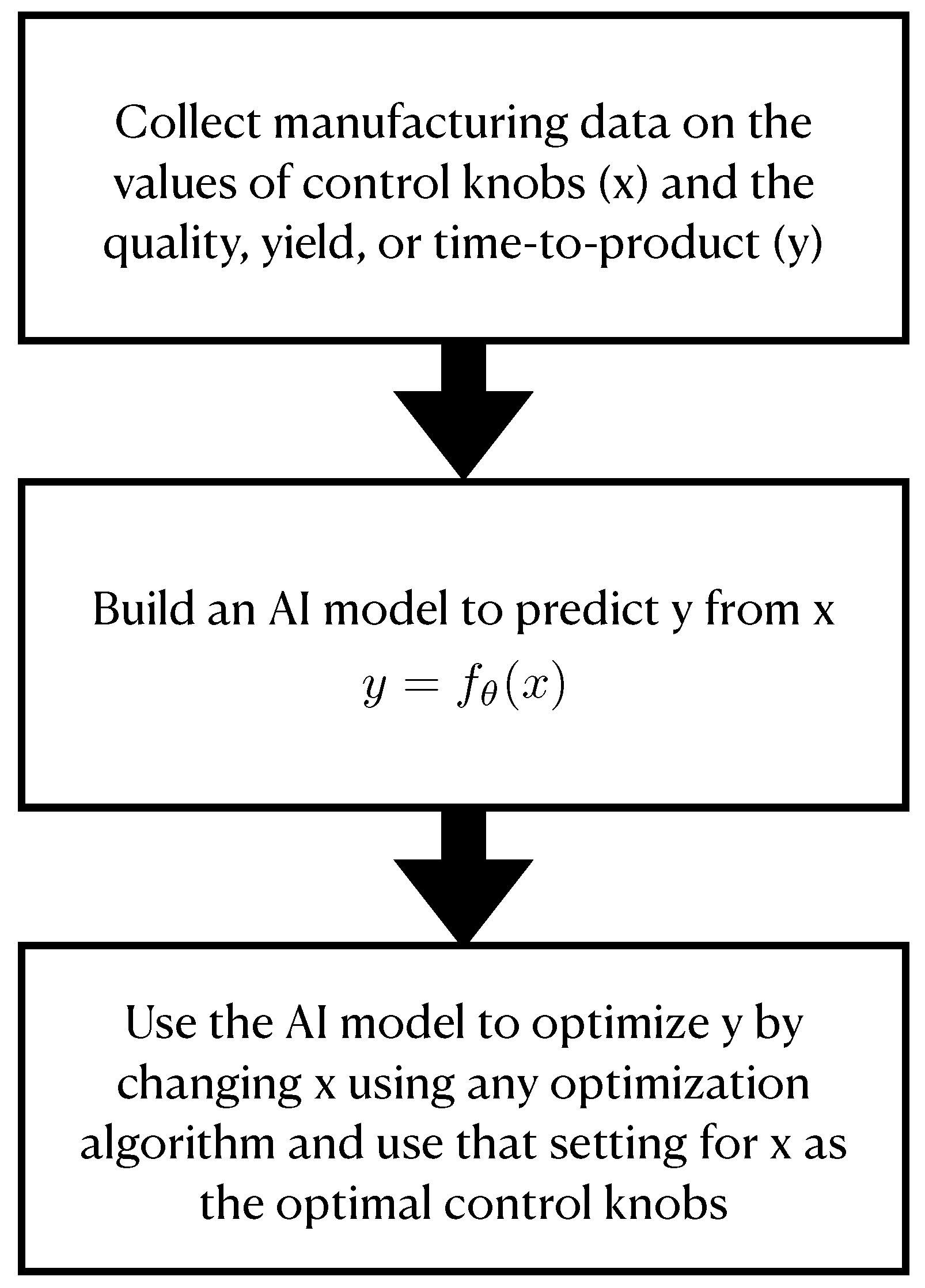
Therefore, our first goal is to model how control knobs affect yield, quality, and time-to-product—using neural networks, support vector machines, or any machine learning algorithm with high predictive accuracy. Second, we propose using standard bounded optimization methods to optimize yield, quality, and/or time-to-product. This results in optimized control knobs that ideally help manufacturers save costs by producing higher-quality goods more efficiently. The generality of this proposal, as well as the new domains to which we envision applying it, are what separates this contribution from previous work. Figure 1 summarizes the two-step procedure after collecting manufacturing data.

Figure 1.
An explanation of the two-step open-loop control procedure proposed to optimize manufacturing processes, resembling the process in Ref. [1] but generalized for application in any manufacturing process. In this manuscript, we focus on wine production, optimizing the product using gradient ascent after building an artificial neural network to predict quality.
This proposal differs from algorithms that detect anomalies [7] or defects [8] in real time during manufacturing. Rather than relying on continuous monitoring to report issues as they happen, our approach focuses on optimizing the manufacturing process upfront using an open-loop method. The open-loop method proposed here could be augmented using smart anomaly and defect detection methods. Our proposal is not a closed-loop method that continually uses a neural network to predict optimal process parameters [9]; instead, we first predict the output of the process and then optimize the process knobs in an open-loop framework.
In this paper, we investigate the conditions under which our proposal is likely to work given noise and finite data, and we apply the method to a dataset on wine quality. Unfortunately, no pharmaceutical manufacturing data (our intended target domain) were available for this study, as such data are not publicly available to our knowledge. Therefore, analysis of this method’s application to pharmaceutical data is reserved for future work.
2. Background
In this section, we review standard supervised learning methods that could easily be used to employ the methods in this paper, and subsequently describe classic optimization algorithms. Together, the two together are the open-loop control method proposed in Figure 1.
2.1. Supervised Learning
The goal of supervised learning is that given x, we aim to produce y. Any black-box model that takes in x and produces an estimate of y that can be tuned is amenable to the method proposed here. We allow x to be multi-dimensional (a vector), but y must be a scalar.
The simplest version of supervised learning would be linear regression for ordinal data and logistic regression for categorical data. Linear regression simply models , while logistic regression models as a softmax applied to . Note that when y is categorical, we optimize the probability that y adopts a particular value—so the second optimization step in the method operates on an ordinal value, not a categorical value. An example of this appears in the Results.
A feedforward artificial neural network (ANN) is an example of an algorithm that, given x, produces for some f and some . For ANNs, the function f depends on how many layers there are in the ANN, how they are connected, the weights and biases (which are the parameters ), and the activation functions in each layer. Recurrent neural networks (RNNs) can also be used; here, we expect x to be a time series input, with an involved repeated f.
For details on how to choose supervised learning models, please see Ref. [10].
2.2. Optimization Algorithms
We would like to eventually maximize the function with respect to x. There are no guarantees about what this function will look like; we only know that takes that form within some boundary. The basic idea behind most optimization methods, if you’re trying to maximize/minimize f, is to ascend/descent the gradient, possibly with additional information about second derivatives or with a momentum term to act as a second derivative.
If is convex, meaning that for any , there is one global minimum, and optimization has been well-understood [11]. Non-convex optimization is an area of research with several methods that recommend it, most of which are implemented in standard numerical software packages, such as Python’s SciPy Optimization v1.16.0 toolkit. For our consideration, any bounded optimization method will do. With non-convex optimization, you are sometimes not guaranteed to find the global minimum or maximum of .
3. Results
We propose a novel two-step method that uses data already collected by manufacturing companies to optimize their processes.
- (1)
- First, we build a machine learning model to predict the desired outcome based on the controllable manufacturing knobs. For instance, in pharmaceutical manufacturing, we might model yield and time-to-product as functions of variables such as chemical concentrations, room temperature, or other control parameters. In other words, let the manufacturing knobs be represented by a vector x, and the property to optimize be y. We then train a model , where represents the model parameters adjusted during training. The universal approximation property guarantees that with enough data on manufacturing knobs, we should be able to build a good model of y using x.
- (2)
- Once we tweak the machine learning model to predict the desired property as accurately as possible, we optimize the desired property, e.g., yield. has now been learned, so we do gradient ascent or any other optimization method to maximize y (or minimize y, depending on what y is) with respect to x, using the aforementioned model within the bounds of the data that existed.
This results in a setting for manufacturing knobs that can optimize the product using artificial intelligence.
First, by combining standard theorems, we confirm this method will work in theory.
Theorem 1.
With enough data, the proposed method can recover the true in order to maximize or minimize the expected output y, within the bounds of x, given by the range of data observed.
Proof
With enough data, we can build an artificial neural network capable of either classification or regression with guaranteed universal approximation, and it will infer for the range of data given the relationship between x and the expected y [12]. Then, convergence proofs for any standard bounded optimization algorithm (such as LFBGS-B [13]) can be applied to maximize or minimize the expected y with respect to x given this inferred relationship. □
To examine this convergence in practice, we use a toy example to illustrate when the method will succeed and fail, with no particular application in mind. Let
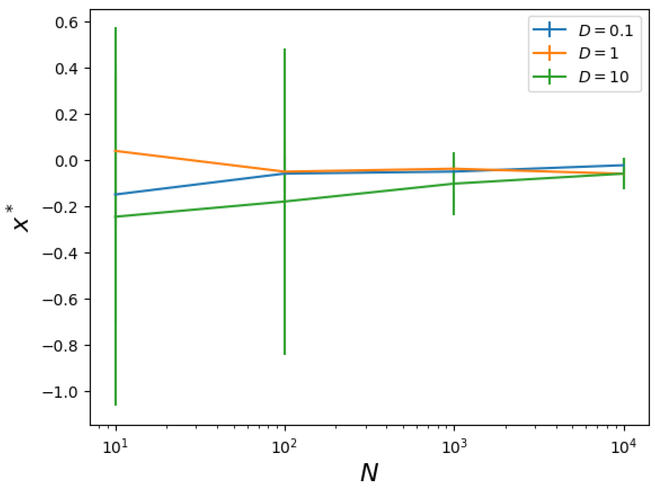
where is a Gaussian noise term with variance D. This example is simplistic, but analytically, we know that the correct solution for minimizing y is to set —which helps us see when this method succeeds and fails. To see if this method can find that , we draw N samples so that our data comprise . Then, is fed to a feedforward ANN with 5 dense layers and 128 neurons in each layer, chosen arbitrarily to be large enough so that universal approximation guarantees should approximately apply [12]. (Activation functions are tanh until the last layer, which is linear.) Once is learned by the feedforward ANN, we perform gradient descent with steps of for 100 iterations to minimize and report ; this is the x returned by the method that minimizes the expected inferred y. In Figure 2, we show as a function of N for various D. As expected, both noise (large D) and finite data (small N) degrade the ability of the method to find the optimal . But, with enough data, i.e., with large enough N, one can find the optimal .

Figure 2.
Proof of principle that the proposed method can find optimal control knobs in the toy example. In the toy example, the optimal control knobs are supposed to be 0. We show the optimal control knobs obtained versus D (noisiness of data) and N (number of data points); this proves that a that a higher N reduces the typical and brings us closer to the true argmin of the expected value of y. Larger amounts of noise move the typical further away from the true argmin.
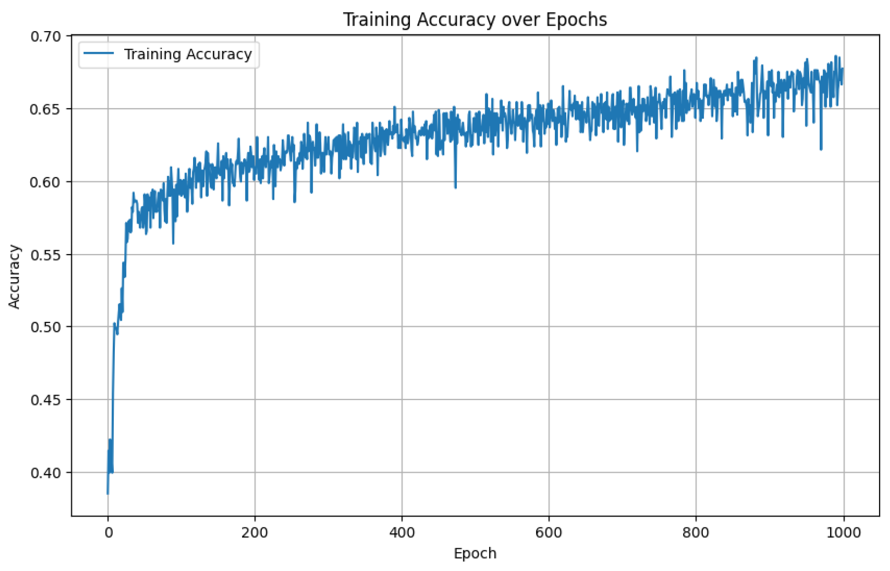
To present a potential use case, we use the publicly available Kaggle dataset of wine properties (fixed acidity, volatile acidity, citric acid, residual sugar, chlorides, free sulfur dioxide, total sulfur dioxide, density, pH, sulphates, and alcohol) that can be controlled by climate, fertilizers, and so on, along with wine quality scores (either 3, 4, 5, 6, 7, 8, or 9). An training/test split was used, leading to roughly 800 data points in the training set. While logistic regression achieved accuracy on the test set and a random forest reached , a simple feedforward ANN—consisting of five dense layers with 64 neurons each, with softmax activations (except for linear activations in the final layer)—achieved accuracy in predicting wine quality on the test set. The ANN used Adam with categorical cross entropy to train. See Figure 3 for an example training curve for accuracy as a function of epochs. Notably, this was not the ANN training curve used to produce the rest of the results given here, as the random initializations were unfortunately not saved from that superior ANN run. Not all datasets in manufacturing will have such low accuracies, e.g., Refs. [14,15].
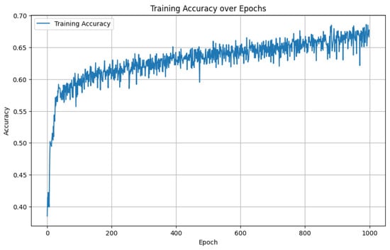
Figure 3.
Classification accuracy increases throughout training for the training set from the wine dataset. Notably, this is a different ANN than the one used to generate other results in the paper.
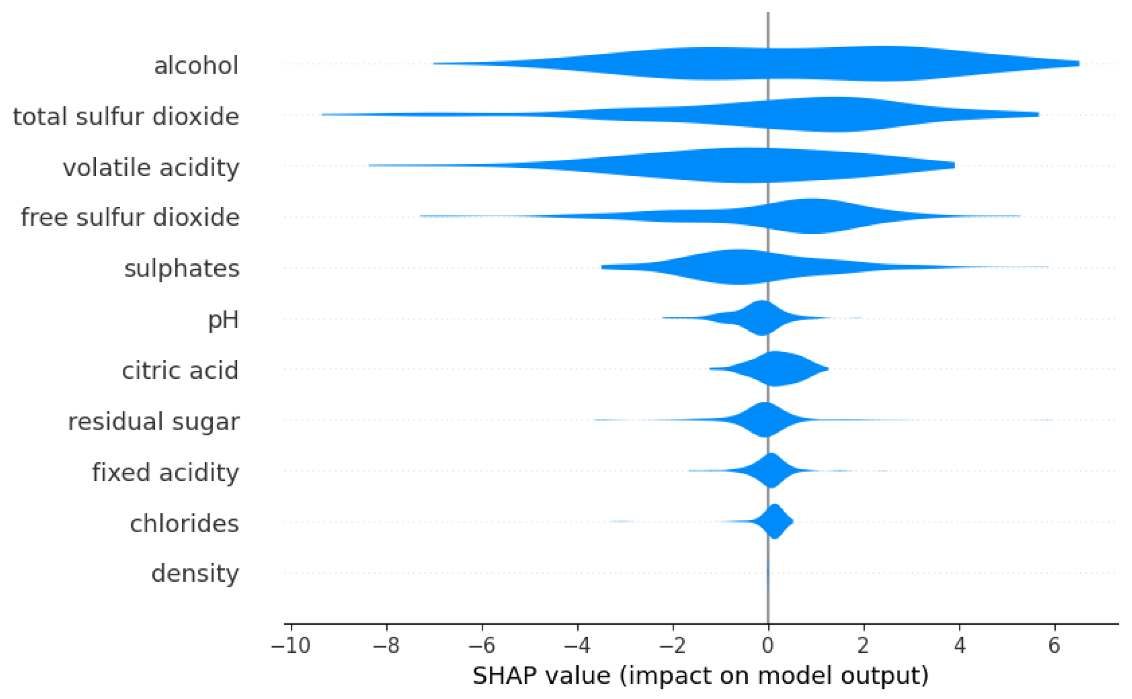
Shapley additive explanation (SHAP) [16] revealed that the main determinant of whether or not the wine was of the highest quality was the alcohol content, followed by the total sulfur dioxide content. See Figure 4. There were seven categories for the quality of wine, so these models are significantly above chance. In general, we expect that manufacturing data for some desired target manufacturing processes may have intrinsic stochasticity that limits the predictive ability of models to less than the accuracies and above often seen in machine learning.

Figure 4.
SHAP [16] values for the importance of features based on the ANN model for determining the probability of having the highest quality wine.
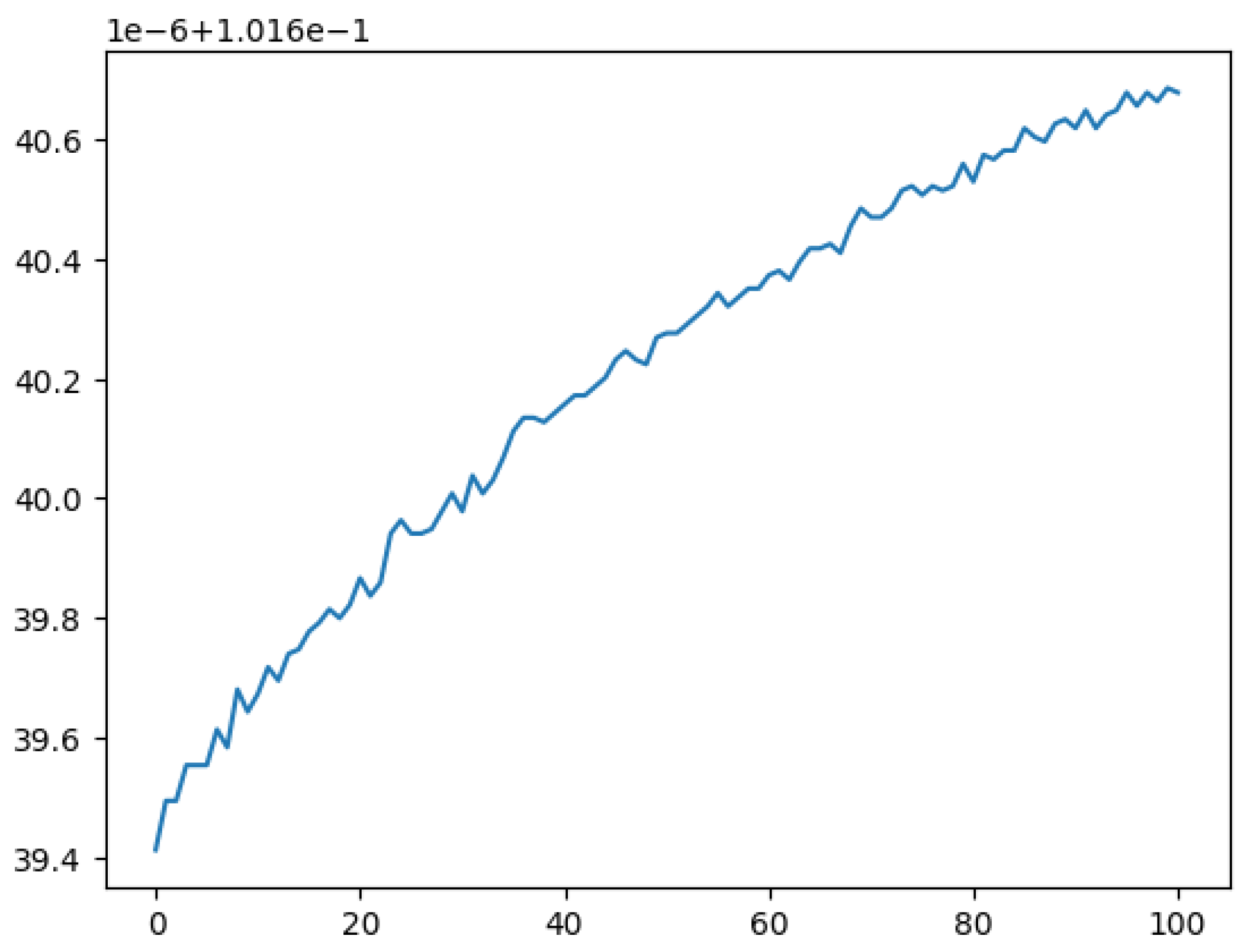
Then, for ANN, a simple bounded gradient ascent algorithm was implemented. Gradients were estimated numerically by taking small steps in every feature and estimating the change in probability itself. To make it a bounded gradient ascent to prevent the model from extrapolating incorrectly, if a gradient step forced one outside the bounds set by the training data, no step was taken. Just 100 steps increased the probability of finding the highest-quality wine, with better results expected from more advanced algorithms for finding maxima that we did not implement here. See Figure 5 for evidence of improvement in the probability of the highest-quality wine score.
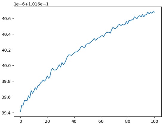
Figure 5.
The probability of the best wine having the highest score improved over even 10 iterations of optimization. On the x-axis is the number of iterations and on the y-axis is the predicted probability of having the highest wine score. The new parameters are approximately: for fixed acidity, for volatile acidity, for citric acid, for residual sugar, for chlorides, for free sulfur dioxide, for total sulfur dioxide, for density, for pH, for sulphates, and for alcohol. If the wine-maker were to make a wine with these parameters, this model suggests it would have a higher wine quality score than the wine they were already making. Further iterations of the optimization would improve this even more.
4. Conclusions
In this work, we proposed a new generalized method for optimizing manufacturing processes. This method is similar to previous methods for circuit card manufacturing monitoring. It involves first building a model of the manufacturing data to predict some target value, whether it be quality or time-to-product or yield, depending on what is appropriate for the industry in question. Then, we use any bounded optimization algorithm to optimize the value of the target that was predicted using the model that was just built. This two-step procedure after collecting manufacturing data is summarized in Figure 1, and is quite general.
For the wine data set used, the appropriate target was the prediction of the quality of the wine. An artificial neural network achieved approximately accuracy for predicting the quality of wine, and even only 100 iterations of gradient ascent improved the likelihood of having the highest quality wine. Further improvements could be expected using improved bounded optimization methods.
5. Discussion
We have shown that, in principle, using toy examples, one can optimize manufacturing processes to minimize the cost of manufacturing and maximize revenue using simple artificial intelligence and optimization ideas. We expect these methods will require some fine-tuning when applied to specific arenas, but that expert knowledge will allow for appropriately structured ANNs and such to be used. We would like to emphasize that the amount of money saved or the additional revenue could be substantial even if there is only a small increase in yield or a small decrease in time-to-product if many products are being made.
It would have been optimal to try this method on many datasets, in particular pharmaceutical manufacturing datasets, but unfortunately, the wine quality dataset was the only publicly available one we could find. We anticipate that future collaborations, hopefully with pharmaceutical companies, could yield further test cases that show the promise of simple artificial intelligence in manufacturing.
This paper essentially generalized the ideas of Ref. [1] to any manufacturing process with improved optimization procedures. In the future, we expect improvements to this method to come from using closed-loop feedback control [17] rather than open-loop feedback, so that intermediate data on the output of the manufacturing system can be taken into account and used to optimize the procedure. This may be difficult to implement immediately in industry given the way that manufacturing processes are often set up, but the extension to closed-loop processes is certainly envisioned after its success in other manufacturing industries [4,18]. In addition, if a model of the process is known, that can be incorporated [19]. We also expect improvements from combining this technique with existing anomaly or defect detection techniques using artificial intelligence that operate in real time.
Funding
This research received no external funding.
Data Availability Statement
Data are available at https://www.kaggle.com/datasets/yasserh/wine-quality-dataset (accessed on 30 June 2025), and all analyses of data are available at https://colab.research.google.com/drive/17D19b-4DSc_issxudV2fqn3jdouHVg25?usp=sharing (accessed on 30 June 2025).
Acknowledgments
We would like to acknowledge Jan Michael Caybayabyab Austria for valuable conversations.
Conflicts of Interest
The author declares no conflicts of interest.
References
- Coit, D.W.; Jackson, B.T.; Smith, A.E. Neural network open loop control system for wave soldering. J. Electron. Manuf. 2002, 11, 95–105. [Google Scholar] [CrossRef]
- Liukkonen, M.; Havia, E.; Hiltunen, Y. Computational intelligence in mass soldering of electronics—A survey. Expert Syst. Appl. 2012, 39, 9928–9937. [Google Scholar] [CrossRef]
- Barajas, L.G. Process Control in High-Noise Environments Using a Limited Number of Measurements; Georgia Institute of Technology: Atlanta, GA, USA, 2003. [Google Scholar]
- Barajas, L.G.; Egerstedt, M.B.; Goldstein, A.; Kamen, E.W. System and Methods for Data-Driven Control of Manufacturing Processes. U.S. Patent 7,171,897, 6 February 2007. [Google Scholar]
- Wuest, T.; Irgens, C.; Thoben, K.D. An approach to monitoring quality in manufacturing using supervised machine learning on product state data. J. Intell. Manuf. 2014, 25, 1167–1180. [Google Scholar] [CrossRef]
- Rai, R.; Tiwari, M.K.; Ivanov, D.; Dolgui, A. Machine learning in manufacturing and industry 4.0 applications. Int. J. Prod. Res. 2021, 59, 4773–4778. [Google Scholar] [CrossRef]
- Singer, G.; Cohen, Y. A framework for smart control using machine-learning modeling for processes with closed-loop control in Industry 4.0. Eng. Appl. Artif. Intell. 2021, 102, 104236. [Google Scholar] [CrossRef]
- Sani, A.R.; Zolfagharian, A.; Kouzani, A.Z. Artificial intelligence-augmented additive manufacturing: Insights on closed-loop 3D printing. Adv. Intell. Syst. 2024, 6, 2400102. [Google Scholar] [CrossRef]
- Thiery, S.; Zein El Abdine, M.; Heger, J.; Ben Khalifa, N. Closed-loop control of product geometry by using an artificial neural network in incremental sheet forming with active medium. Int. J. Mater. Form. 2021, 14, 1319–1335. [Google Scholar] [CrossRef]
- Mehta, P.; Bukov, M.; Wang, C.H.; Day, A.G.; Richardson, C.; Fisher, C.K.; Schwab, D.J. A high-bias, low-variance introduction to machine learning for physicists. Phys. Rep. 2019, 810, 1–124. [Google Scholar] [CrossRef] [PubMed]
- Boyd, S. Convex Optimization; Cambridge University Press: Cambridge, UK, 2004. [Google Scholar]
- Hornik, K.; Stinchcombe, M.; White, H. Multilayer feedforward networks are universal approximators. Neural Netw. 1989, 2, 359–366. [Google Scholar] [CrossRef]
- Gao, W.; Goldfarb, D. Quasi-Newton methods: Superlinear convergence without line searches for self-concordant functions. Optim. Methods Softw. 2019, 34, 194–217. [Google Scholar] [CrossRef]
- Jin, W.; Pei, J.; Xie, P.; Chen, J.; Zhao, H. Machine learning-based prediction of mechanical properties and performance of nickel–graphene nanocomposites using molecular dynamics simulation data. ACS Appl. Nano Mater. 2023, 6, 12190–12199. [Google Scholar] [CrossRef]
- Yang, L.; Wang, H.; Leng, D.; Fang, S.; Yang, Y.; Du, Y. Machine learning applications in nanomaterials: Recent advances and future perspectives. Chem. Eng. J. 2024, 500, 156687. [Google Scholar] [CrossRef]
- Lundberg, S.M.; Lee, S.I. A unified approach to interpreting model predictions. arXiv 2017, arXiv:1705.07874. [Google Scholar]
- Åström, K.J.; Murray, R. Feedback Systems: An Introduction for Scientists and Engineers; Princeton University Press: Princeton, NJ, USA, 2021. [Google Scholar]
- Jiang, S.; Zeng, Y.; Zhu, Y.; Pou, J.; Konstantinou, G. Stability-oriented multiobjective control design for power converters assisted by deep reinforcement learning. IEEE Trans. Power Electron. 2023, 38, 12394–12400. [Google Scholar] [CrossRef]
- Xiao, Z.; Zeng, Y.; Tang, Y. Swift and seamless start-up of dab converters in constant and variable frequency modes. IEEE Trans. Ind. Electron. 2024, 72, 4763–4775. [Google Scholar] [CrossRef]
Disclaimer/Publisher’s Note: The statements, opinions and data contained in all publications are solely those of the individual author(s) and contributor(s) and not of MDPI and/or the editor(s). MDPI and/or the editor(s) disclaim responsibility for any injury to people or property resulting from any ideas, methods, instructions or products referred to in the content. |
© 2025 by the author. Licensee MDPI, Basel, Switzerland. This article is an open access article distributed under the terms and conditions of the Creative Commons Attribution (CC BY) license (https://creativecommons.org/licenses/by/4.0/).