

MSP-EDA: Multivariate Time Series Forecasting Based on Multiscale Patches and External Data Augmentation

 ,
,  and
and
Abstract
1. Introduction
- We design an adaptive multiscale wavelet-based representation module that automatically adjusts scale decomposition based on the characteristics of input data, enabling the model to extract rich and relevant time–frequency features.
- We introduce a cross-attention that dynamically fuses external data, enhancing the ability to adapt to complex and changing input conditions.
- We propose a novel MSP-EDA framework, which unifies multiscale patch representation and external data integration to capture complex temporal patterns and intra-variable dependencies.
- We perform extensive experiments on seven benchmark datasets to demonstrate that MSP-EDA consistently outperforms state-of-the-art baselines, confirming its effectiveness and generalizability across diverse forecasting scenarios.
2. Related Work
2.1. Multivariate Time Series Forecasting
2.2. Multiscale Modeling for MTS Forecasting
2.3. MTS Forecasting with External Data
3. Methodology
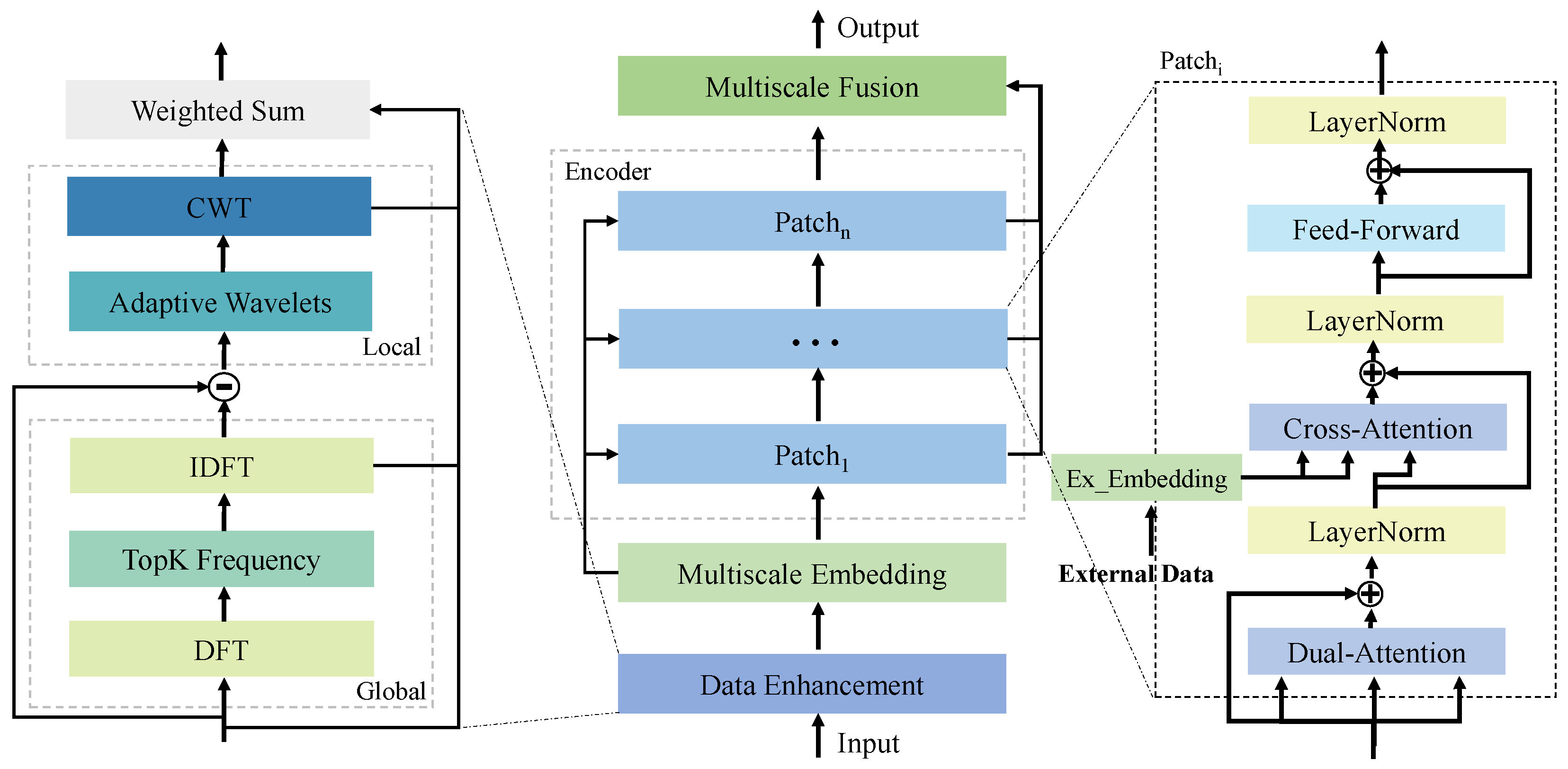
3.1. Overview
- Data Pattern Enhancement: Extracts both global periodic trends and localized time–frequency features using signal processing techniques, specifically leveraging the Discrete Fourier Transform (DFT) to identify dominant global frequency components and the Continuous Wavelet Transform (CWT) to capture localized, non-stationary patterns across time and scale.
- Multiscale Patch Processing: Decomposes the time series into multiple temporal resolutions to capture multiscale dependencies while simultaneously modeling temporal dynamics and inter-variable correlations. In addition, tailored embedding strategies are designed to effectively integrate external data into each scale for enhanced contextual understanding.
- Multiscale Fusion: Combines representations from different temporal scales by introducing a global variable token, which is fused with the outputs from each encoder layer to generate the final prediction. This process effectively integrates multiscale information and external data, ensuring a comprehensive representation for accurate forecasting.
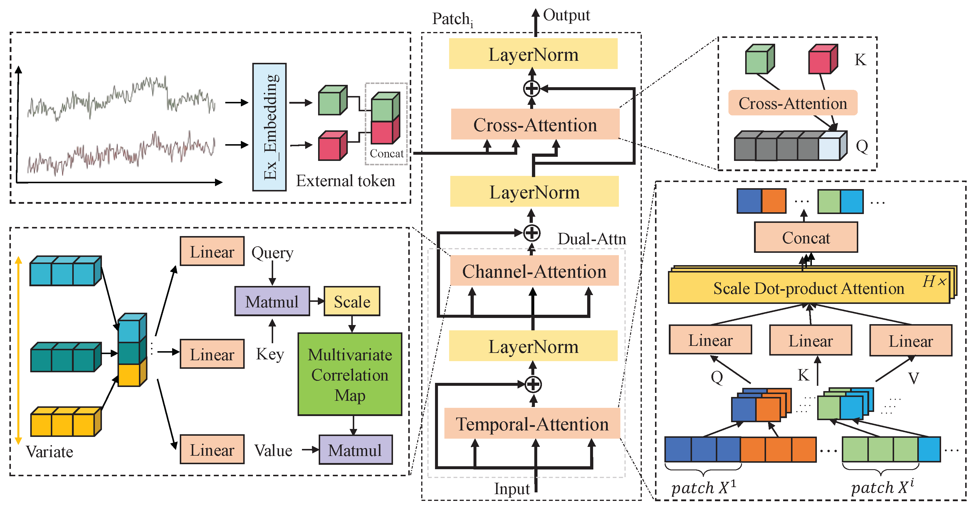
3.2. Data Pattern Enhancement
3.3. Multiscale Patch Processing
3.4. Multiscale Fusion
4. Experiments
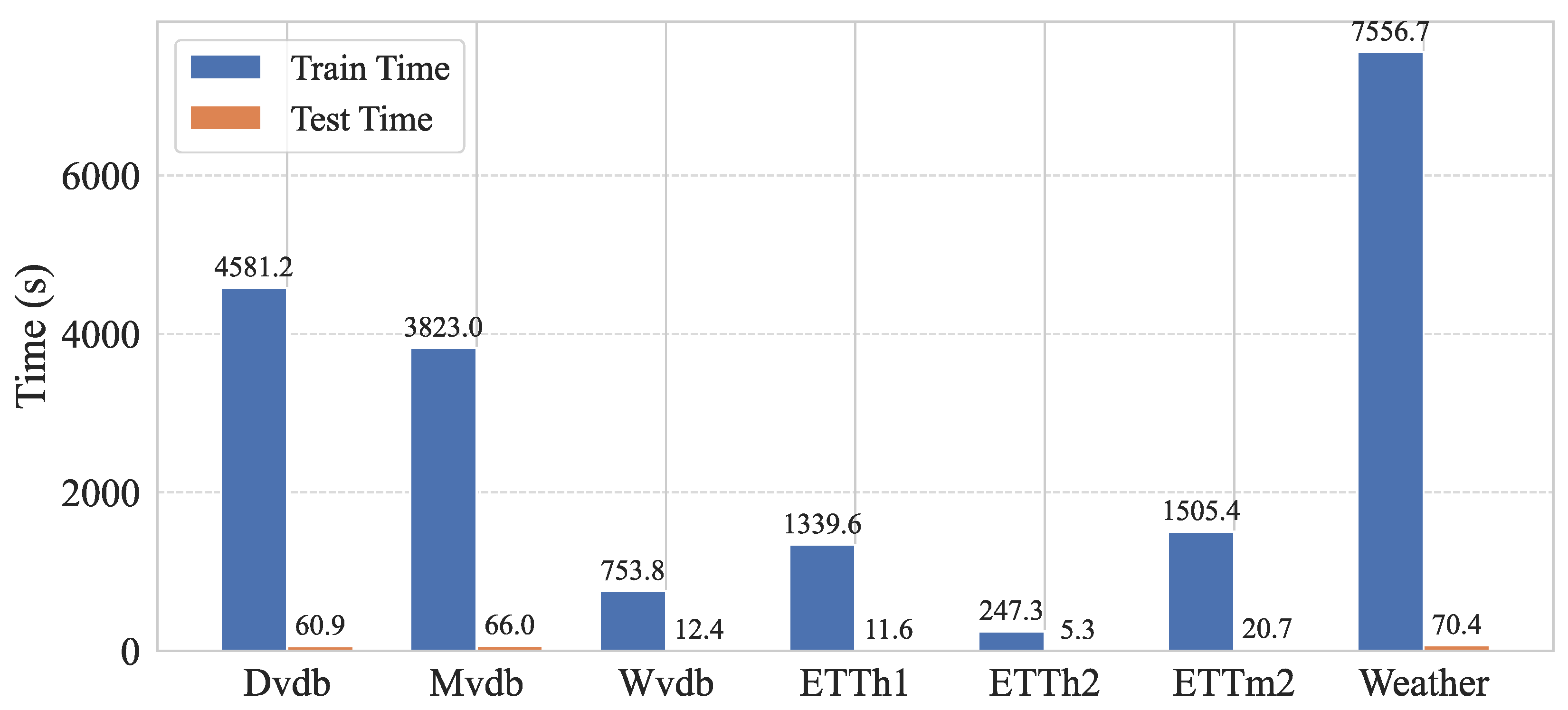
4.1. Experimental Setup
4.2. Overall Performance
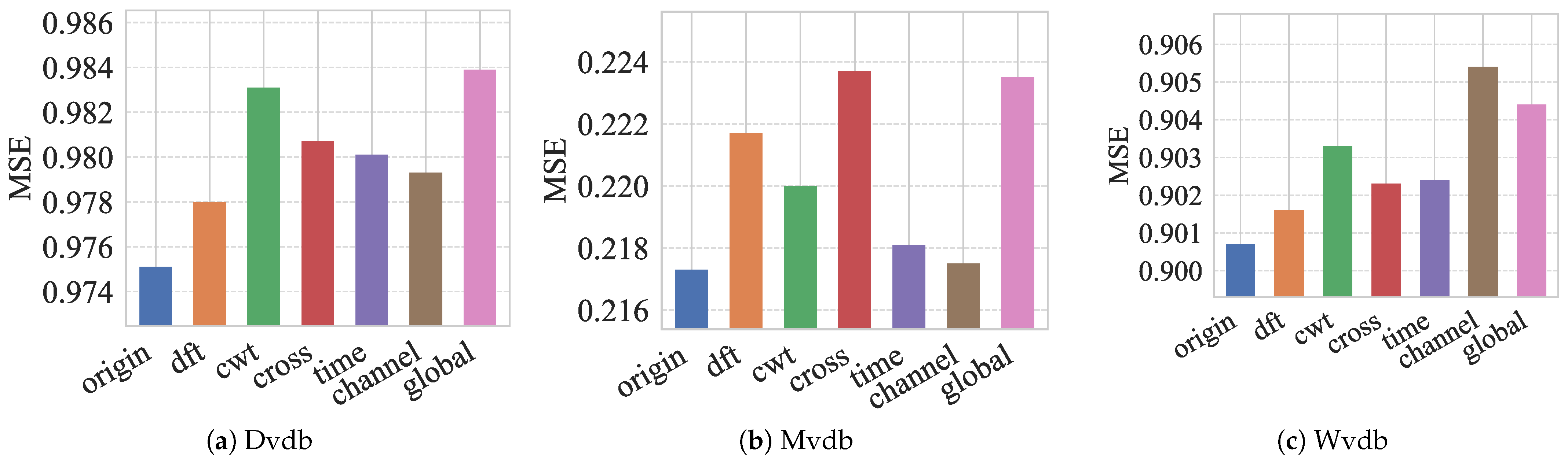
4.3. Ablation Study
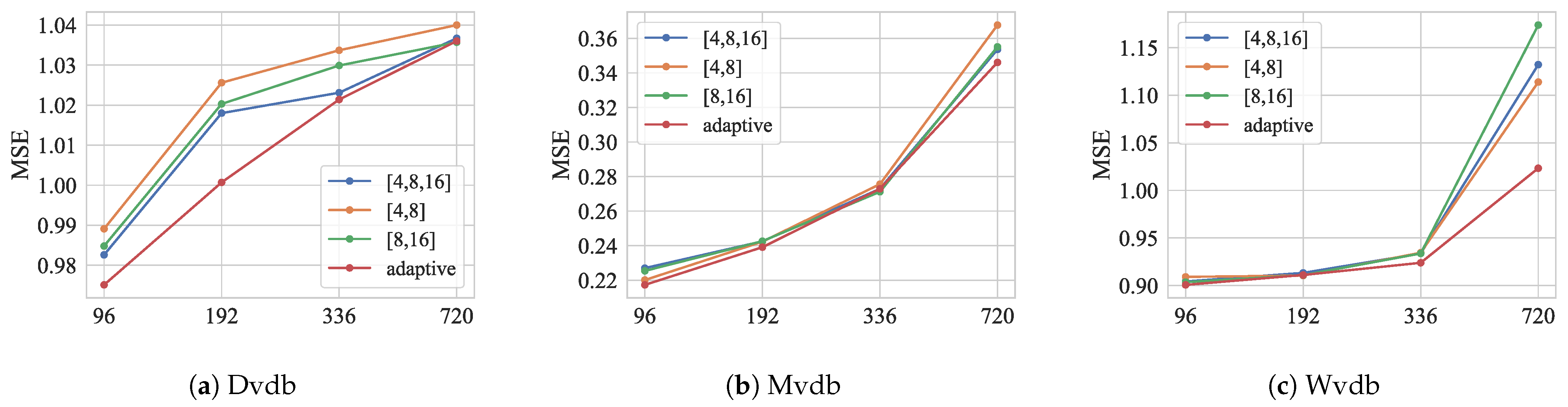
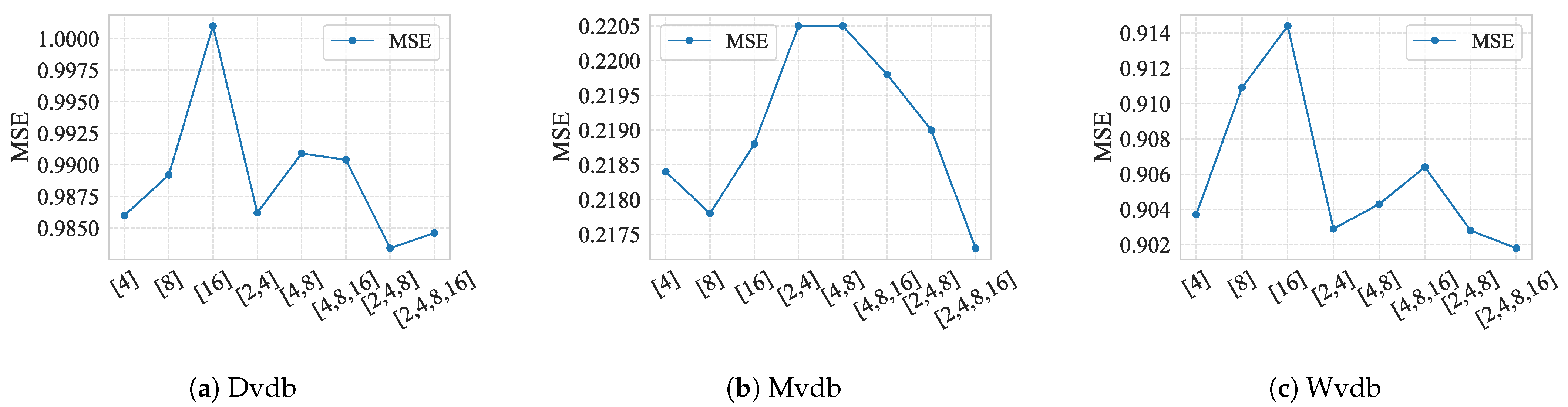
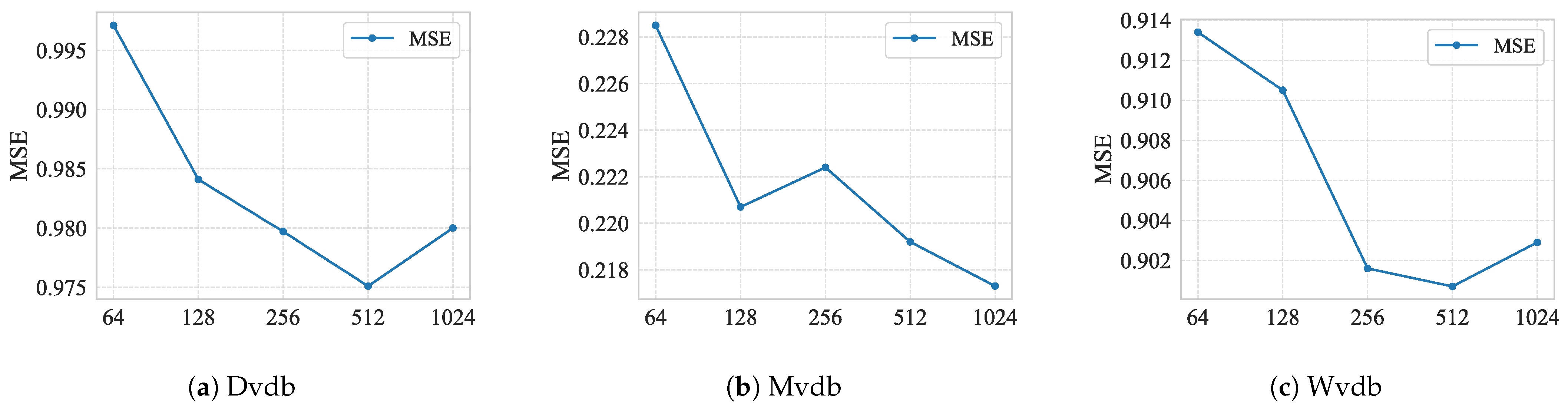
4.4. Hyperparameter Analysis
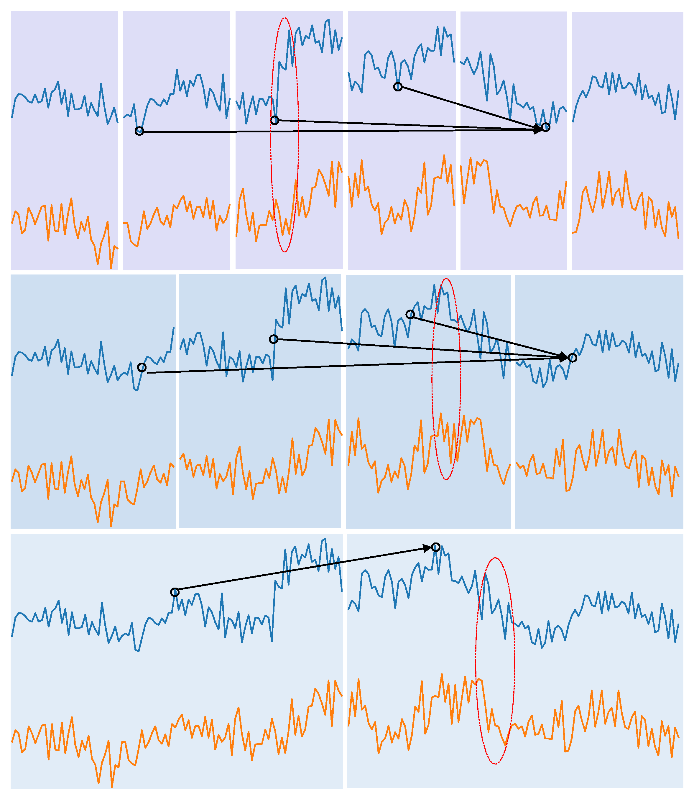
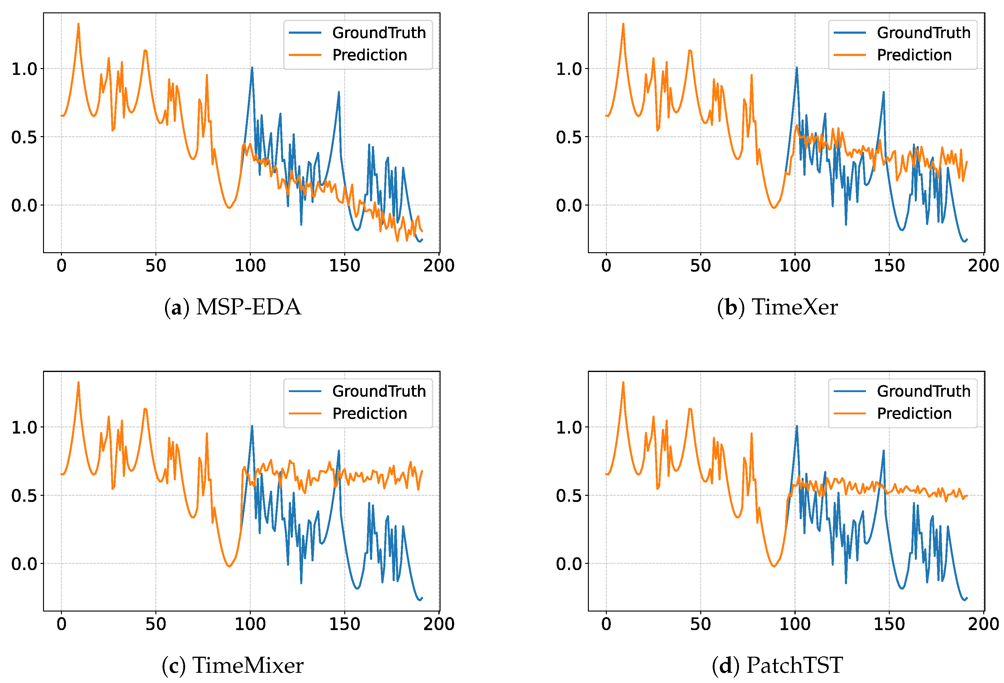
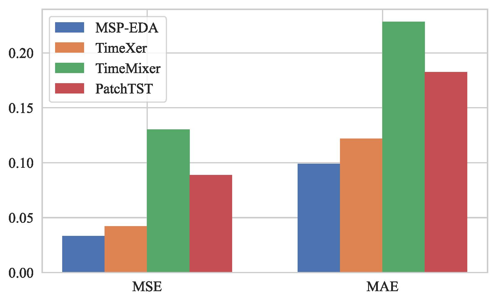
4.5. Visualization
5. Conclusions
Author Contributions
Funding
Data Availability Statement
Conflicts of Interest
References
- Sezer, O.B.; Gudelek, M.U.; Ozbayoglu, A.M. Financial time series forecasting with deep learning: A systematic literature review: 2005–2019. Appl. Soft Comput. 2020, 90, 106181. [Google Scholar] [CrossRef]
- Lin, Y.; Wan, H.; Guo, S.; Lin, Y. Pre-training context and time aware location embeddings from spatial-temporal trajectories for user next location prediction. Proc. AAAI Conf. Artif. Intell. 2021, 35, 4241–4248. [Google Scholar] [CrossRef]
- Sun, C.; Ning, Y.; Shen, D.; Nie, T. Graph Neural Network-Based Short-Term Load Forecasting with Temporal Convolution. Data Sci. Eng. 2024, 9, 113–132. [Google Scholar] [CrossRef]
- Miao, X.; Wu, Y.; Wang, J.; Gao, Y.; Mao, X.; Yin, J. Generative semi-supervised learning for multivariate time series imputation. Proc. AAAI Conf. Artif. Intell. 2021, 35, 8983–8991. [Google Scholar] [CrossRef]
- Wang, Y.; Huang, N.; Li, T.; Yan, Y.; Zhang, X. Medformer: A Multi-Granularity Patching Transformer for Medical Time-Series Classification. Adv. Neural Inf. Process. Syst. 2024, 37, 36314–36341. [Google Scholar]
- Pan, Z.; Wang, Y.; Zhang, Y.; Yang, S.B.; Cheng, Y.; Chen, P.; Guo, C.; Wen, Q.; Tian, X.; Dou, Y.; et al. MagicScaler: Uncertainty-Aware, Predictive Autoscaling. Proc. VLDB Endow. 2023, 16, 3808–3821. [Google Scholar] [CrossRef]
- Wang, S.; Chu, Z.; Sun, Y.; Liu, Y.; Guo, Y.; Chen, Y.; Jian, H.; Ma, L.; Lu, X.; Zhou, J. Multiscale Representation Enhanced Temporal Flow Fusion Model for Long-Term Workload Forecasting. In Proceedings of the 33rd ACM International Conference on Information and Knowledge Management, New York, NY, USA, 21–25 October 2024; pp. 4948–4956. [Google Scholar] [CrossRef]
- Zhao, F.; Lin, W.; Lin, S.; Zhong, H.; Li, K. TFEGRU: Time-Frequency Enhanced Gated Recurrent Unit with Attention for Cloud Workload Prediction. IEEE Trans. Serv. Comput. 2024, 18, 467–478. [Google Scholar] [CrossRef]
- Gao, Y.; Huang, X.; Zhou, X.; Gao, X.; Li, G.; Chen, G. DBAugur: An Adversarial-based Trend Forecasting System for Diversified Workloads. In Proceedings of the 39th IEEE International Conference on Data Engineering, Anaheim, CA, USA, 3–7 April 2023; pp. 27–39. [Google Scholar] [CrossRef]
- Guo, Y.; Ge, J.; Guo, P.; Chai, Y.; Li, T.; Shi, M.; Tu, Y.; Ouyang, J. Pass: Predictive auto-scaling system for large-scale enterprise web applications. In Proceedings of the ACM Web Conference 2024, Singapore, 13–17 May 2024; pp. 2747–2758. [Google Scholar] [CrossRef]
- Kilian, L.; Lütkepohl, H. Structural Vector Autoregressive Analysis; Cambridge University Press: Cambridge, UK, 2017. [Google Scholar] [CrossRef]
- Lin, S.; Lin, W.; Wu, W.; Zhao, F.; Mo, R.; Zhang, H. SegRNN: Segment Recurrent Neural Network for Long-Term Time Series Forecasting. arXiv 2023, arXiv:2308.11200. Available online: https://arxiv.org/abs/2308.11200 (accessed on 22 May 2025).
- Liu, M.; Zeng, A.; Chen, M.; Xu, Z.; Lai, Q.; Ma, L.; Xu, Q. SCINet: Time Series Modeling and Forecasting with Sample Convolution and Interaction. Adv. Neural Inf. Process. Syst. 2022, 35, 5816–5828. [Google Scholar]
- Liu, Y.; Hu, T.; Zhang, H.; Wu, H.; Wang, S.; Ma, L.; Long, M. iTransformer: Inverted Transformers Are Effective for Time Series Forecasting. In Proceedings of the Twelfth International Conference on Learning Representations, Vienna, Austria, 7–11 May 2024; Available online: https://openreview.net/forum?id=JePfAI8fah (accessed on 22 May 2025).
- Wang, Y.; Wu, H.; Dong, J.; Qin, G.; Zhang, H.; Liu, Y.; Qiu, Y.; Wang, J.; Long, M. TimeXer: Empowering Transformers for Time Series Forecasting with Exogenous Variables. Adv. Neural Inf. Process. Syst. 2024, 37, 469–498. [Google Scholar]
- Zhou, H.; Zhang, S.; Peng, J.; Zhang, S.; Li, J.; Xiong, H.; Zhang, W. Informer: Beyond efficient transformer for long sequence time-series forecasting. Proc. AAAI Conf. Artif. Intell. 2021, 35, 11106–11115. [Google Scholar] [CrossRef]
- Wu, H.; Xu, J.; Wang, J.; Long, M. Autoformer: Decomposition Transformers with Auto-Correlation for Long-Term Series Forecasting. Adv. Neural Inf. Process. Syst. 2021, 34, 22419–22430. [Google Scholar]
- Zhou, T.; Ma, Z.; Wen, Q.; Wang, X.; Sun, L.; Jin, R. Fedformer: Frequency enhanced decomposed transformer for long-term series forecasting. In Proceedings of the 39th International Conference on Machine Learning, 17–23 July 2022; Volume 162, pp. 27268–27286. Available online: https://proceedings.mlr.press/v162/zhou22g/zhou22g.pdf (accessed on 22 May 2025).
- Bandara, K.; Hyndman, R.J.; Bergmeir, C. MSTL: A seasonal-trend decomposition algorithm for time series with multiple seasonal patterns. Int. J. Oper. Res. 2025, 52, 79–98. [Google Scholar] [CrossRef]
- Wen, Q.; Zhang, Z.; Li, Y.; Sun, L. Fast RobustSTL: Efficient and Robust Seasonal-Trend Decomposition for Time Series with Complex Patterns. In Proceedings of the 26th ACM SIGKDD International Conference on Knowledge Discovery & Data Mining, New York, NY, USA, 6–10 June 2020; pp. 2203–2213. [Google Scholar] [CrossRef]
- Fan, W.; Yi, K.; Ye, H.; Ning, Z.; Zhang, Q.; An, N. Deep frequency derivative learning for non-stationary time series forecasting. In Proceedings of the Thirty-Third International Joint Conference on Artificial Intelligence, Jeju, Republic of Korea, 3–9 August 2024; pp. 3944–3952. [Google Scholar] [CrossRef]
- Xu, Z.; Zeng, A.; Xu, Q. FITS: Modeling Time Series with $10k$ Parameters. In Proceedings of the Twelfth International Conference on Learning Representations, Vienna, Austria, 7–11 May 2024; Available online: https://openreview.net/forum?id=bWcnvZ3qMb (accessed on 22 May 2025).
- Ye, W.; Deng, S.; Zou, Q.; Gui, N. Frequency Adaptive Normalization For Non-stationary Time Series Forecasting. Adv. Neural Inf. Process. Syst. 2024, 37, 31350–31379. [Google Scholar]
- Qiu, X.; Hu, J.; Zhou, L.; Wu, X.; Du, J.; Zhang, B.; Guo, C.; Zhou, A.; Jensen, C.S.; Sheng, Z.; et al. TFB: Towards Comprehensive and Fair Benchmarking of Time Series Forecasting Methods. Proc. VLDB Endow. 2024, 17, 2363–2377. [Google Scholar] [CrossRef]
- Zhang, Y.; Yan, J. Crossformer: Transformer Utilizing Cross-Dimension Dependency for Multivariate Time Series Forecasting. In Proceedings of the Eleventh International Conference on Learning Representations, Kigali, Rwanda, 1–5 May 2023; Available online: https://openreview.net/forum?id=vSVLM2j9eie (accessed on 22 May 2025).
- Zhong, S.; Song, S.; Zhuo, W.; Li, G.; Liu, Y.; Chan, S.H.G. A Multi-Scale Decomposition MLP-Mixer for Time Series Analysis. Proc. VLDB Endow. 2024, 17, 1723–1736. [Google Scholar] [CrossRef]
- Chen, P.; ZHANG, Y.; Cheng, Y.; Shu, Y.; Wang, Y.; Wen, Q.; Yang, B.; Guo, C. Pathformer: Multi-scale Transformers with Adaptive Pathways for Time Series Forecasting. In Proceedings of the Twelfth International Conference on Learning Representations, Vienna, Austria, 7–11 May 2024; Available online: https://openreview.net/forum?id=lJkOCMP2aW (accessed on 22 May 2025).
- Lee, S.; Park, T.; Lee, K. Learning to Embed Time Series Patches Independently. In Proceedings of the Twelfth International Conference on Learning Representations, Vienna, Austria, 7–11 May 2024; Available online: https://openreview.net/forum?id=WS7GuBDFa2 (accessed on 22 May 2025).
- Nie, Y.; Nguyen, N.H.; Sinthong, P.; Kalagnanam, J. A Time Series is Worth 64 Words: Long-term Forecasting with Transformers. In Proceedings of the Eleventh International Conference on Learning Representations, Kigali, Rwanda, 1–5 May 2023; Available online: https://openreview.net/forum?id=Jbdc0vTOcol (accessed on 22 May 2025).
- Cai, W.; Liang, Y.; Liu, X.; Feng, J.; Wu, Y. MSGNet: Learning Multi-Scale Inter-Series Correlations for Multivariate Time Series Forecasting. Proc. AAAI Conf. Artif. Intell. 2024, 38, 11141–11149. [Google Scholar] [CrossRef]
- Williams, B.M. Multivariate vehicular traffic flow prediction: Evaluation of ARIMAX modeling. Transp. Res. Rec. 2001, 1776, 194–200. [Google Scholar] [CrossRef]
- Das, A.; Kong, W.; Leach, A.; Mathur, S.K.; Sen, R.; Yu, R. Long-term Forecasting with TiDE: Time-series Dense Encoder. Trans. Mach. Learn. Res. 2023. Available online: https://openreview.net/forum?id=pCbC3aQB5W (accessed on 22 May 2025).
- Shumway, R.H.; Stoffer, D.S.; Shumway, R.H.; Stoffer, D.S. ARIMA models. Time Series Analysis and Its Applications: With R Examples; Springer: Cham, Switzerland, 2017; pp. 75–163. [Google Scholar] [CrossRef]
- Wu, H.; Hu, T.; Liu, Y.; Zhou, H.; Wang, J.; Long, M. TimesNet: Temporal 2D-Variation Modeling for General Time Series Analysis. In Proceedings of the Eleventh International Conference on Learning Representations, Kigali, Rwanda, 1–5 May 2023; Available online: https://openreview.net/forum?id=ju_Uqw384Oq (accessed on 22 May 2025).
- Salinas, D.; Flunkert, V.; Gasthaus, J.; Januschowski, T. DeepAR: Probabilistic forecasting with autoregressive recurrent networks. Int. J. Forecast. 2020, 36, 1181–1191. [Google Scholar] [CrossRef]
- Wang, S.; Wu, H.; Shi, X.; Hu, T.; Luo, H.; Ma, L.; Zhang, J.Y.; ZHOU, J. TimeMixer: Decomposable Multiscale Mixing for Time Series Forecasting. In Proceedings of the Twelfth International Conference on Learning Representations, Vienna, Austria, 7–11 May 2024; Available online: https://openreview.net/forum?id=7oLshfEIC2 (accessed on 22 May 2025).
- Zeng, A.; Chen, M.; Zhang, L.; Xu, Q. Are transformers effective for time series forecasting? Proc. AAAI Conf. Artif. Intell. 2023, 37, 11121–11128. [Google Scholar] [CrossRef]
- Li, Y.; Wu, C.Y.; Fan, H.; Mangalam, K.; Xiong, B.; Malik, J.; Feichtenhofer, C. MViTv2: Improved Multiscale Vision Transformers for Classification and Detection. In Proceedings of the 2022 IEEE/CVF Conference on Computer Vision and Pattern Recognition, New Orleans, LA, USA, 18–24 June 2022; pp. 4794–4804. [Google Scholar] [CrossRef]
- Wang, J.; Wu, Z.; Ouyang, W.; Han, X.; Chen, J.; Jiang, Y.G.; Li, S.N. M2TR: Multi-modal Multi-scale Transformers for Deepfake Detection. In Proceedings of the 2022 International Conference on Multimedia Retrieval, New York, NY, USA, 27–30 June 2022; pp. 615–623. [Google Scholar] [CrossRef]
- Challu, C.; Olivares, K.G.; Oreshkin, B.N.; Ramirez, F.G.; Canseco, M.M.; Dubrawski, A. NHITS: Neural Hierarchical Interpolation for Time Series Forecasting. Proc. AAAI Conf. Artif. Intell. 2023, 37, 6989–6997. [Google Scholar] [CrossRef]
- Shabani, M.A.; Abdi, A.H.; Meng, L.; Sylvain, T. Scaleformer: Iterative Multi-scale Refining Transformers for Time Series Forecasting. In Proceedings of the The Eleventh International Conference on Learning Representations, Kigali, Rwanda, 1–5 May 2023; Available online: https://openreview.net/forum?id=sCrnllCtjoE (accessed on 22 May 2025).
- Zhang, Y.; Ma, L.; Pal, S.; Zhang, Y.; Coates, M. Multi-resolution Time-Series Transformer for Long-term Forecasting. In Proceedings of the 27th International Conference on Artificial Intelligence and Statistics, Valencia, Spain, 2–4 May 2024; Volume 238, pp. 4222–4230. Available online: https://proceedings.mlr.press/v238/zhang24l/zhang24l.pdf (accessed on 22 May 2025).
- Arunraj, N.S.; Ahrens, D.; Fernandes, M. Application of SARIMAX model to forecast daily sales in food retail industry. Int. J. Oper. Res. Inf. Syst. 2016, 7, 1–21. [Google Scholar] [CrossRef]
- Lim, B.; Arık, S.O.; Loeff, N.; Pfister, T. Temporal Fusion Transformers for interpretable multi-horizon time series forecasting. Int. J. Forecast. 2021, 37, 1748–1764. [Google Scholar] [CrossRef]
- Olivares, K.G.; Challu, C.; Marcjasz, G.; Weron, R.; Dubrawski, A. Neural basis expansion analysis with exogenous variables: Forecasting electricity prices with NBEATSx. Int. J. Forecast. 2023, 39, 884–900. [Google Scholar] [CrossRef]
- Wang, H.; Peng, J.; Huang, F.; Wang, J.; Chen, J.; Xiao, Y. MICN: Multi-scale Local and Global Context Modeling for Long-term Series Forecasting. In Proceedings of the Eleventh International Conference on Learning Representations, Kigali, Rwanda, 1–5 May 2023; Available online: https://openreview.net/forum?id=zt53IDUR1U (accessed on 22 May 2025).
- Su, Y.; Tan, M.; Teh, J. Short-Term Transmission Capacity Prediction of Hybrid Renewable Energy Systems Considering Dynamic Line Rating Based on Data-Driven Model. IEEE Trans. Ind. Appl. 2025, 61, 2410–2420. [Google Scholar] [CrossRef]
- Kim, J.; Kim, H.; Kim, H.; Lee, D.; Yoon, S. A Comprehensive Survey of Time Series Forecasting: Architectural Diversity and Open Challenges. arXiv 2024, arXiv:2411.05793. Available online: https://arxiv.org/abs/2411.05793 (accessed on 22 May 2025).

| Method | Decomposition | Multiscale | External Data |
|---|---|---|---|
| FEDformer [18] | ✓ | × | × |
| MICN [46] | ✓ | ✓ | × |
| TiDE [32] | × | ✓ | ✓ |
| MSGNet [30] | ✓ | ✓ | × |
| MSD-Mixer [26] | ✓ | ✓ | × |
| Pathformer [27] | ✓ | ✓ | × |
| TimeXer [15] | × | × | ✓ |
| MSP-EDA (This work) | ✓ | ✓ | ✓ |
| Dataset | Dimension | Timestamps | Granularity |
|---|---|---|---|
| ETTh1 | 7 | 17,420 | 1 h |
| ETTh2 | 7 | 17,420 | 1 h |
| ETTm2 | 7 | 69,680 | 15 min |
| Weather | 21 | 52,696 | 10 min |
| Dvdb | 22 | 28,278 | 1 min |
| Mvdb | 18 | 21,570 | 1 min |
| Wvdb | 15 | 18,490 | 1 min |
| Model | MSP-EDA | TimeXer | TimeMixer | HRTCP | TimesNet | PatchTST | TiDE | FEDformer | |||||||||
|---|---|---|---|---|---|---|---|---|---|---|---|---|---|---|---|---|---|
| Metric | MSE | MAE | MSE | MAE | MSE | MAE | MSE | MAE | MSE | MAE | MSE | MAE | MSE | MAE | MSE | MAE | |
| ETTh1 | 96 | 0.3771 | 0.4034 | 0.3873 | 0.4057 | 0.3865 | 0.4011 | 0.3883 | 0.4032 | 0.3931 | 0.4145 | 0.3916 | 0.4103 | 0.3888 | 0.3968 | 0.3801 | 0.4196 |
| 192 | 0.4277 | 0.4332 | 0.4399 | 0.4278 | 0.4425 | 0.4323 | 0.5213 | 0.4873 | 0.5483 | 0.4958 | 0.4371 | 0.4298 | 0.4401 | 0.4260 | 0.4694 | 0.4693 | |
| 336 | 0.4655 | 0.4565 | 0.4798 | 0.4483 | 0.4768 | 0.4556 | 0.5533 | 0.5013 | 0.5564 | 0.5062 | 0.4784 | 0.4524 | 0.4834 | 0.4486 | 0.5231 | 0.4908 | |
| 720 | 0.4792 | 0.4803 | 0.4876 | 0.4747 | 0.5334 | 0.4920 | 0.5910 | 0.5325 | 0.7257 | 0.6046 | 0.4770 | 0.4753 | 0.4861 | 0.4735 | 0.5365 | 0.5153 | |
| ETTh2 | 96 | 0.2910 | 0.3403 | 0.2952 | 0.3425 | 0.3001 | 0.3519 | 0.2954 | 0.3438 | 0.3293 | 0.3695 | 0.2940 | 0.3509 | 0.2912 | 0.3404 | 0.3470 | 0.3894 |
| 192 | 0.3745 | 0.4013 | 0.3703 | 0.3930 | 0.3768 | 0.3964 | 0.3937 | 0.4008 | 0.4657 | 0.4516 | 0.3685 | 0.3937 | 0.3765 | 0.3919 | 0.4154 | 0.4251 | |
| 336 | 0.4171 | 0.4326 | 0.4228 | 0.4340 | 0.4438 | 0.4450 | 0.4445 | 0.4467 | 0.5046 | 0.4852 | 0.4158 | 0.4298 | 0.4221 | 0.4301 | 0.4624 | 0.4697 | |
| 720 | 0.4382 | 0.4504 | 0.4474 | 0.4553 | 0.4482 | 0.4584 | 0.4613 | 0.4699 | 0.4925 | 0.4842 | 0.4272 | 0.4483 | 0.4232 | 0.4417 | 0.4819 | 0.4866 | |
| ETTm2 | 96 | 0.1730 | 0.2597 | 0.1759 | 0.2579 | 0.1754 | 0.2601 | 0.1801 | 0.2613 | 0.1895 | 0.2686 | 0.1833 | 0.2671 | 0.1822 | 0.2650 | 0.2006 | 0.2849 |
| 192 | 0.2383 | 0.3016 | 0.2364 | 0.2999 | 0.2448 | 0.3051 | 0.2480 | 0.3080 | 0.2547 | 0.3110 | 0.2511 | 0.3107 | 0.2487 | 0.3057 | 0.2639 | 0.3221 | |
| 336 | 0.2976 | 0.3395 | 0.2952 | 0.3385 | 0.3023 | 0.3475 | 0.3155 | 0.3602 | 0.3150 | 0.3492 | 0.3126 | 0.3487 | 0.3075 | 0.3430 | 0.3278 | 0.3628 | |
| 720 | 0.3998 | 0.3999 | 0.3965 | 0.3980 | 0.3951 | 0.4013 | 0.4218 | 0.4179 | 0.4211 | 0.4080 | 0.4124 | 0.4038 | 0.4077 | 0.3984 | 0.4169 | 0.4132 | |
| Weather | 96 | 0.1609 | 0.2089 | 0.1576 | 0.2049 | 0.1618 | 0.2088 | 0.1732 | 0.2086 | 0.1694 | 0.2187 | 0.1709 | 0.2122 | 0.1930 | 0.2343 | 0.2108 | 0.2900 |
| 192 | 0.2105 | 0.2535 | 0.2115 | 0.2531 | 0.2070 | 0.2513 | 0.2211 | 0.2532 | 0.2390 | 0.2779 | 0.2287 | 0.2617 | 0.2400 | 0.2700 | 0.2640 | 0.3169 | |
| 336 | 0.2645 | 0.2922 | 0.2668 | 0.2931 | 0.2911 | 0.3095 | 0.2968 | 0.3156 | 0.2897 | 0.3110 | 0.2832 | 0.3003 | 0.2919 | 0.3062 | 0.3144 | 0.3470 | |
| 720 | 0.3436 | 0.3438 | 0.3436 | 0.3433 | 0.3430 | 0.3439 | 0.3781 | 0.3724 | 0.3590 | 0.3539 | 0.3592 | 0.3497 | 0.3652 | 0.3540 | 0.3815 | 0.3828 | |
| Dvdb | 96 | 0.9751 | 0.7130 | 0.9889 | 0.7137 | 0.9817 | 0.7154 | 0.9892 | 0.7194 | 1.0789 | 0.7546 | 0.9924 | 0.7214 | 1.047 | 0.7455 | 1.0726 | 0.7686 |
| 192 | 1.0007 | 0.7273 | 1.0191 | 0.7389 | 1.0080 | 0.7281 | 1.0273 | 0.7405 | 1.0808 | 0.7535 | 1.0359 | 0.7462 | 1.1658 | 0.7963 | 1.0964 | 0.7752 | |
| 336 | 1.0214 | 0.7365 | 1.0382 | 0.7412 | 1.0282 | 0.7339 | 1.0521 | 0.7453 | 1.0968 | 0.7598 | 1.0587 | 0.7566 | 1.1893 | 0.8058 | 1.1154 | 0.7833 | |
| 720 | 1.0360 | 0.7454 | 1.0490 | 0.7493 | 1.0362 | 0.7463 | 1.0913 | 0.7707 | 1.1034 | 0.7623 | 1.0768 | 0.7650 | 1.1983 | 0.8104 | 1.1219 | 0.7855 | |
| Mvdb | 96 | 0.2173 | 0.2968 | 0.2219 | 0.2978 | 0.2342 | 0.3060 | 0.2312 | 0.2997 | 0.2474 | 0.3101 | 0.2357 | 0.3008 | 0.2564 | 0.3131 | 0.2448 | 0.3143 |
| 192 | 0.2391 | 0.3114 | 0.2403 | 0.3146 | 0.2781 | 0.3349 | 0.2638 | 0.3199 | 0.2547 | 0.3227 | 0.2676 | 0.3313 | 0.3072 | 0.3512 | 0.2736 | 0.3366 | |
| 336 | 0.2729 | 0.3465 | 0.2774 | 0.3452 | 0.3286 | 0.3694 | 0.3256 | 0.3688 | 0.2854 | 0.3490 | 0.3145 | 0.3652 | 0.3540 | 0.3837 | 0.3227 | 0.3724 | |
| 720 | 0.3461 | 0.3956 | 0.3752 | 0.4066 | 0.4479 | 0.4351 | 0.4503 | 0.4337 | 0.3767 | 0.4107 | 0.4271 | 0.4299 | 0.4659 | 0.4446 | 0.4364 | 0.4380 | |
| Wvdb | 96 | 0.9007 | 0.5913 | 0.9178 | 0.5978 | 0.9192 | 0.5989 | 0.9213 | 0.6007 | 0.9391 | 0.6041 | 0.9095 | 0.5974 | 0.9593 | 0.6141 | 0.9419 | 0.6128 |
| 192 | 0.9111 | 0.6055 | 0.9196 | 0.6089 | 0.9509 | 0.6245 | 0.9324 | 0.6096 | 0.9347 | 0.6161 | 0.9239 | 0.6157 | 1.0970 | 0.6657 | 0.9386 | 0.6225 | |
| 336 | 0.9239 | 0.6274 | 0.9330 | 0.6288 | 0.9833 | 0.6530 | 0.9617 | 0.6458 | 0.9527 | 0.6363 | 0.9445 | 0.6392 | 1.1218 | 0.6902 | 0.9562 | 0.6450 | |
| 720 | 1.0233 | 0.6908 | 1.1054 | 0.7031 | 1.0723 | 0.7097 | 1.0617 | 0.7113 | 1.1270 | 0.7189 | 1.1249 | 0.7086 | 1.1995 | 0.7461 | 1.0371 | 0.7021 | |
Disclaimer/Publisher’s Note: The statements, opinions and data contained in all publications are solely those of the individual author(s) and contributor(s) and not of MDPI and/or the editor(s). MDPI and/or the editor(s) disclaim responsibility for any injury to people or property resulting from any ideas, methods, instructions or products referred to in the content. |
© 2025 by the authors. Licensee MDPI, Basel, Switzerland. This article is an open access article distributed under the terms and conditions of the Creative Commons Attribution (CC BY) license (https://creativecommons.org/licenses/by/4.0/).
Share and Cite
Peng, S.; Sun, W.; Chen, P.; Xu, H.; Ma, D.; Chen, M.; Wang, Y.; Li, H. MSP-EDA: Multivariate Time Series Forecasting Based on Multiscale Patches and External Data Augmentation. Electronics 2025, 14, 2618. https://doi.org/10.3390/electronics14132618
Peng S, Sun W, Chen P, Xu H, Ma D, Chen M, Wang Y, Li H. MSP-EDA: Multivariate Time Series Forecasting Based on Multiscale Patches and External Data Augmentation. Electronics. 2025; 14(13):2618. https://doi.org/10.3390/electronics14132618
Chicago/Turabian StylePeng, Shunhua, Wu Sun, Panfeng Chen, Huarong Xu, Dan Ma, Mei Chen, Yanhao Wang, and Hui Li. 2025. "MSP-EDA: Multivariate Time Series Forecasting Based on Multiscale Patches and External Data Augmentation" Electronics 14, no. 13: 2618. https://doi.org/10.3390/electronics14132618
APA StylePeng, S., Sun, W., Chen, P., Xu, H., Ma, D., Chen, M., Wang, Y., & Li, H. (2025). MSP-EDA: Multivariate Time Series Forecasting Based on Multiscale Patches and External Data Augmentation. Electronics, 14(13), 2618. https://doi.org/10.3390/electronics14132618