Equivalent Loop Bandwidth of Kalman Filter-Based Tracking Method

Abstract

Digital phase-locked loop (DPLL) is currently the most commonly used for carrier tracking, and its performance can be easily evaluated by the loop bandwidth. Meanwhile, the Kalman filter-based tracking (KFT) method has been widely studied to further improve the tracking performance; however, there is no analytical expression to describe the relationship between the parameters of KFT and its performance. To solve this problem, the consistency between the two techniques is established in the paper by approximating the innovations of the Kalman filter. Based on that, the equivalent loop bandwidth of the KFT method is derived, which could be used for KFT accurate performance evaluation and efficient parameter optimization.

1. Introduction

Stable carrier tracking of received signals is fundamental in communication systems [1], satellite navigation [2], and radar [3]. The digital phase-locked loop (DPLL) which was derived from the traditional analog phase-locked loop is currently the most commonly used technology for carrier tracking because of its simplicity in implementation scheme and parameter design [4].

The power of GNSS (Global Navigation Satellite System) signal is extremely weak, making carrier tracking in a challenge environment particularly difficult. As is well known, the Kalman filter is optimal for parameter estimation [5]. To further improve the carrier tracking performance including tracking accuracy and dynamic adaptability, numerous Kalman filter-based tracking (KFT) methods optimized for specific scenarios have been studied, including: enhancing tracking sensitivity in a weak signal environment [6,7,8,9], improving dynamic adaptability under high-dynamic conditions [10,11,12], enhancing tracking stability during ionospheric scintillation [13,14,15,16], and improving availability during signal outages [17,18]. Besides being used for the carrier tracking, the Kalman filter has also been used for frequency estimation [19], and extensively applied in emerging areas such as industrial IoT [20], UAVs [21], and the Internet of Vehicles [22].

In addition to proposing novel algorithms, tracking accuracy and dynamic adaptability, which are two conflicting aspects of tracking performance, could be improved by parameter optimization according to specific scenarios. In the design of DPLL, according to the analytical expression, the minimum loop bandwidth satisfying dynamic adaptability or the maximum loop bandwidth satisfying tracking accuracy could be calculated to optimize the other aspect of tracking performance [23]. However, the impact of KFT parameters including process noise and observation noise on tracking performance has not been analytically described currently, resulting in inefficient parameter adjustment based on experience [24]. Since tracking accuracy and dynamic adaptability are two conflicting aspects of tracking performance, tracking accuracy should be compared under the same dynamic adaptability, or dynamic adaptability should be compared under the same tracking accuracy. However, different types of parameters are used in KFT and DPLL which make it difficult to accurately compare their performance. The link between the two types of parameters in KFT and DPLL needs to be established for a fair comparison.

Although various carrier tracking methods based on the Kalman filter have been proposed, few papers have studied their theoretical performance. Reference [25] analyzes the similarities and differences in transfer function and transient response between KFT and DPLL, with detailed listings. The results show that the KFT exhibits a shorter transient time, which coincides with conclusions drawn in [26]. However, the performance of KFT still cannot be quantitatively evaluated according to these conclusions. The equivalent loop bandwidth of KFT method under steady-state conditions is derived in [27,28], but a Kalman filter model without feedback was used for analysis, which diverges significantly from the actual process of carrier tracking.

To analytically evaluate KFT performance and make accurate comparisons with DPLL under identical conditions, the analytical expression of the equivalent loop bandwidth of KFT, based on the error feedback model that aligns with the actual carrier tracking process, is derived for the first time. Finally, numerical simulation results are given to validate the conclusion.

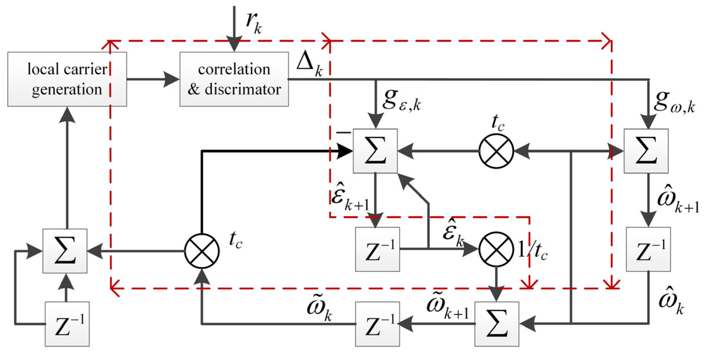
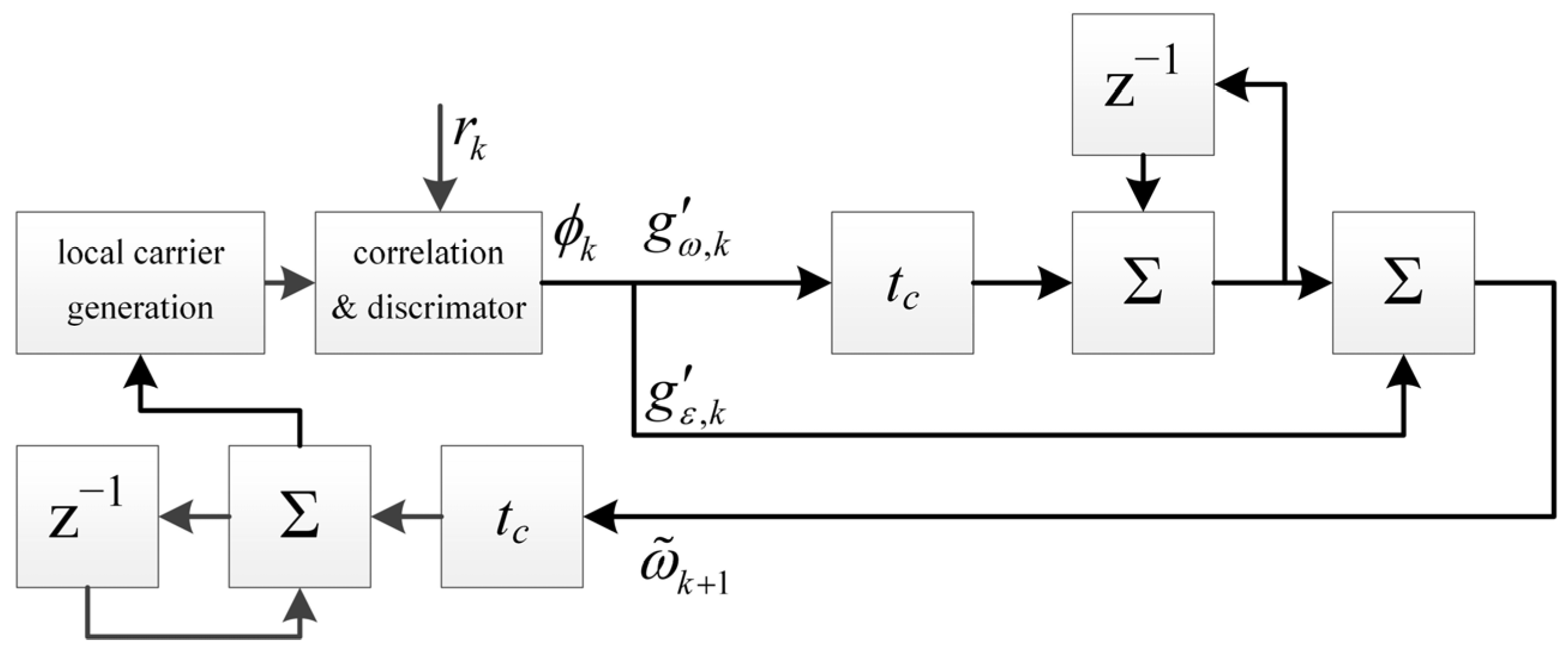
2. Mathematical Model of KFT Method

The model of the baseband signal without modulated symbol is used below for simplification. In the KFT method, the continuous signal is firstly divided into multiple segments with a period of $t_c$. When only the first-order dynamic is considered, the signal for each segment $r_k\left(t\right)$ could be modeled as

$$r_k\left(t\right)=\sqrt{2C}{\mathrm{e}}^{\mathrm{j}\left({\omega }_{k}t+{\theta }_{0,k}\right)}+n\left(t\right),0\le t\le t_c$$

(1)

where ${\theta }_{0,k}$ and ${\omega }_k$ are the initial carrier phase and the Doppler frequency during the time interval $\left[k{t}_c,\left(k+1\right)t_c\right]$ respectively.

It follows that the initial carrier phase and Doppler frequency in adjacent periods satisfy the following relationship:

$$\left[\begin{array}{c}{\theta }_{0,k+1}\\ {\omega }_{k+1}\end{array}\right]=\left[\begin{array}{cc}1& t_c\\ 0& 1\end{array}\right]\left[\begin{array}{c}{\theta }_{0,k}\\ {\omega }_k\end{array}\right]+\left[\begin{array}{c}0\\ w_{\omega ,k}\end{array}\right]$$

(2)

where $w_{\omega ,k}$ represents jitter in the Doppler frequency, which follows a zero mean Gaussian distribution with a variance of ${\sigma }_{\omega }^2$.

The initial carrier phase difference between the received and local signal rather than the initial carrier phase is estimated in the KFT method. In a common GNSS receiver, the local signal, also in first-order dynamic form, is generated for correlation, and only the Doppler frequency is adjusted in carrier tracking. Based on the aforementioned limitations, from (2), the relationship of initial carrier phase error ${\epsilon }_k$ between different periods can be modeled as follows:

$$\begin{array}{ll}{\epsilon }_{k+1}& ={\theta }_{0,k+1}-{\tilde{\theta }}_{0,k+1}\\ & ={\omega }_k{t}_c+{\theta }_{0,k}-\left({\tilde{\omega }}_k{t}_c+{\tilde{\theta }}_{0,k}\right)\\ & ={\omega }_k{t}_c+{\epsilon }_k-{\tilde{\omega }}_k{t}_c\end{array}$$

(3)

where ${\tilde{\theta }}_{0,k}$ and ${\tilde{\omega }}_k$ represent the initial phase and the Doppler frequency of the local signal during the time interval $\left[k{t}_c,\left(k+1\right)t_c\right]$, respectively.

The state transition equation of the KFT method can be modeled as:

$${\mathit{x}}_{k+1}=\mathsf{\Phi }{\mathit{x}}_k-{\mathit{u}}_k+{\mathit{w}}_k$$

(4)

where ${\mathit{x}}_k={\left[\begin{array}{cc}{\epsilon }_k& {\omega }_k\end{array}\right]}^{\mathrm{T}}$ is the state vector, ${\mathit{u}}_k={\left[\begin{array}{cc}{\tilde{\omega }}_k{t}_c& 0\end{array}\right]}^{\mathrm{T}}$ represents the external input for the KFT method, $\mathsf{\Phi }$ denotes the state transition matrix, and ${\mathit{w}}_k={\left[\begin{array}{cc}0& w_{\omega ,k}\end{array}\right]}^{\mathrm{T}}$ indicates the process noise with a covariance matrix of $\mathbf{Q}$. The expressions for $\mathsf{\Phi }$ and $\mathbf{Q}$ are as follows:

$$\mathbf{Q}=\left[\begin{array}{cc}0& 0\\ 0& {\sigma }_{\omega }^2\end{array}\right],\mathsf{\Phi }=\left[\begin{array}{cc}1& t_c\\ 0& 1\end{array}\right]$$

(5)

The phase difference between the local signal $s_k\left(t\right)$ and the received signal $r_k\left(t\right)$ could be estimated by the correlation value $y_k$, whose expression is

$$\begin{array}{ll}{y}_k& ={\displaystyle \frac{1}{t_c}}{\displaystyle {\int }_0^{t_c}{r}_k\left(t\right)s_k^{*}\left(t\right)dt}\\ & =\sqrt{2C}\mathrm{sinc}\left({\omega }_{\Delta ,k}{t}_c/2\right){\mathrm{e}}^{\mathrm{j}\left({\omega }_{\Delta ,k}{t}_c/2+{\epsilon }_k\right)}+n_{y,k}\end{array}$$

(6)

where ${\omega }_{\Delta ,k}={\omega }_k-{\tilde{\omega }}_k$ represents the Doppler frequency difference, and $n_{y,k}$ denotes the noise component in the correlation value, $s_k^{*}\left(t\right)$ means the conjugation of $s_k\left(t\right)$.

When the half cycle ambiguity is not considered, the relationship between the carrier phase discriminator output and the state vector is as follows:

$$\begin{array}{ll}{\varphi }_k& ={\tan }^{-1}\left\{\mathrm{Im}\left(y_k\right)/\mathrm{Re}\left(y_k\right)\right\}\\ & =\left[\begin{array}{cc}1& t_c/2\end{array}\right]\left[\begin{array}{c}{\epsilon }_k\\ {\omega }_k\end{array}\right]-{\tilde{\omega }}_k{t}_c/2+v_{\varphi ,k}\end{array}$$

(7)

where $\mathrm{R}\mathrm{e}\left(y\right)$ and $\mathrm{I}\mathrm{m}\left(y\right)$ denote the real and imaginary part of y, respectively, $v_{\varphi ,k}$ represents the observation noise, which follows a zero mean Gaussian distribution with a variance of ${\sigma }_{\varphi }^2$.

Based on (7), the observation equation can be modeled as follows:

$$z_k=\mathbf{H}{\mathit{x}}_k+v_{\varphi ,k}$$

(8)

where $z_k={\varphi }_k+{\tilde{\omega }}_k{t}_c/2$ represents the observation vector, and $\mathbf{H}=\left[\begin{array}{cc}1& t_c/2\end{array}\right]$ represents the observation matrix.

Based on (4) and (8), the update of the state vector could be expressed as follows:

$$\begin{array}{ll}{\widehat{\mathit{x}}}_{k+1}& =\left(\mathsf{\Phi }{\widehat{\mathit{x}}}_k-{\mathit{u}}_k\right)+{\mathbf{G}}_{k+1}\left[z_{k+1}-\mathbf{H}\left(\mathsf{\Phi }{\widehat{\mathit{x}}}_k-{\mathit{u}}_k\right)\right]\\ & \triangleq \left(\mathsf{\Phi }{\widehat{\mathit{x}}}_k-{\mathit{u}}_k\right)+{\mathbf{G}}_{k+1}{\Delta }_{k+1}\end{array}$$

(9)

where ${\widehat{\mathit{x}}}_{k+1}$ and ${\widehat{\mathit{x}}}_k={\left[\begin{array}{cc}{\widehat{\epsilon }}_k& {\widehat{\omega }}_k\end{array}\right]}^{\mathrm{T}}$ represent the optimal estimates of the state vectors ${\mathit{x}}_{k+1}$ and ${\mathit{x}}_k$, respectively, ${\Delta }_{k+1}$ denotes the innovation in the period $\left[\left(k+1\right)t_c,\left(k+2\right)t_c\right]$, and ${\mathbf{G}}_k={\left[\begin{array}{cc}{g}_{\epsilon ,k}& g_{\omega ,k}\end{array}\right]}^{\mathrm{T}}$ represents the gain matrix. Assuming the covariance matrix of the state vector is ${\mathbf{P}}_k$, the update of the gain matrix ${\mathbf{G}}_k$ could be expressed as follows:

$${\mathbf{G}}_k={\mathbf{P}}_k{\mathbf{H}}_k^{\mathrm{T}}/{\sigma }_{\varphi }^2$$

(10)

$${\mathbf{P}}_k^{-1}={\left(\mathsf{\Phi }{\mathbf{P}}_{k-1}{\mathsf{\Phi }}^T+\mathbf{Q}\right)}^{-1}+{\mathbf{H}}^T\mathbf{H}/{\sigma }_{\varphi }^2$$

(11)

Equation (9) can be expressed with matrix elements as follows

$$\left[\begin{array}{c}{\widehat{\epsilon }}_{k+1}\\ {\widehat{\omega }}_{k+1}\end{array}\right]=\left[\begin{array}{cc}1& t_c\\ 0& 1\end{array}\right]\left[\begin{array}{c}{\widehat{\epsilon }}_k\\ {\widehat{\omega }}_k\end{array}\right]-\left[\begin{array}{c}{\tilde{\omega }}_k{t}_c\\ 0\end{array}\right]+\left[\begin{array}{c}{g}_{\epsilon ,k+1}\\ g_{\omega ,k+1}\end{array}\right]{\Delta }_{k+1}$$

(12)

The form of Doppler frequency ${\tilde{\omega }}_k$ in (12) is not unique, and the solution which makes ${\epsilon }_{k+1}$ in (3) equal 0 is used here, which is

$${\tilde{\omega }}_{k+1}={\widehat{\omega }}_k+{\widehat{\epsilon }}_k/t_c$$

(13)

Equations (12) and (13) are the mathematical model of the KFT method, and its implementation block diagram is shown in Figure 1. The red dashed arrows indicate the data flow direction in the loop.

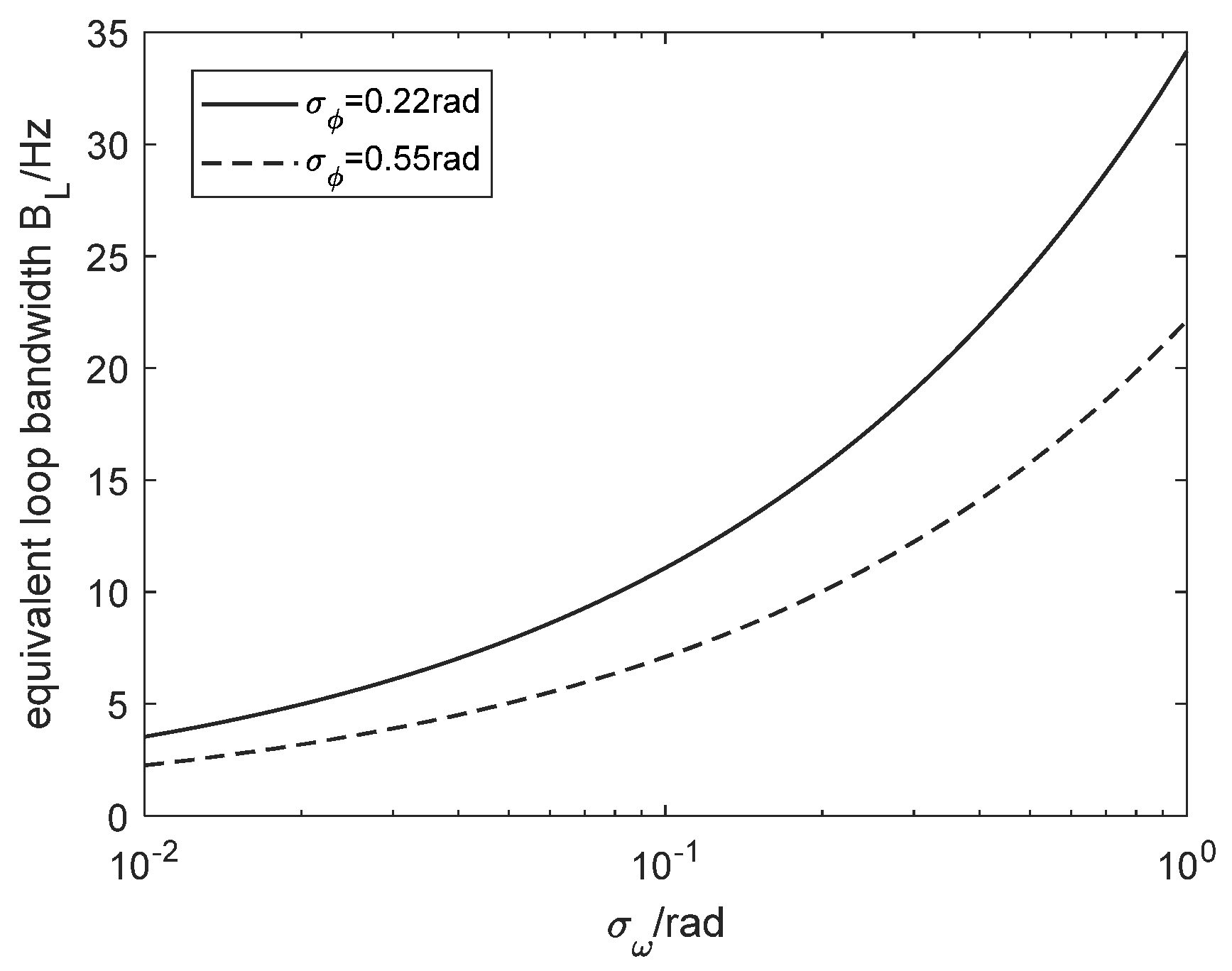
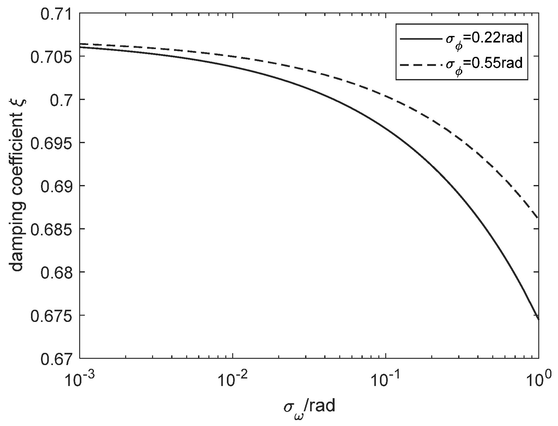
3. Equivalent Loop Bandwidth of KFT Method

The loop bandwidth of DPLL is the most important parameter, which directly determines the thermal noise error and dynamic adaptation. Meanwhile, the parameters of the KFT method are the process noise variance ${\sigma }_{\omega }^2$ and the observation noise variance ${\sigma }_{\phi }^2$, which are different from those of DPLL. Therefore, to enable accurate performance comparison under identical conditions between KFT and DPLL, the equivalent loop bandwidth of the KFT method must be derived. In the following, the theoretical expression of the equivalent loop bandwidth of KFT is derived.

According to (9), the innovation ${\Delta }_{k+1}$ in (12) could be expressed as

$${\Delta }_{k+1}={\varphi }_{k+1}-{\displaystyle \frac{3}{2}}{\widehat{\omega }}_k{t}_c-{\widehat{\epsilon }}_k+{\displaystyle \frac{1}{2}}{\tilde{\omega }}_{k+1}{t}_c+{\tilde{\omega }}_k{t}_c$$

(14)

When the Doppler frequency changes slowly, ${\widehat{\omega }}_k$ and ${\widehat{\omega }}_{k-1}$ approximately equal. Under stable carrier tracking conditions, ${\widehat{\epsilon }}_k$ approximately equals 0. Furthermore, from (13), ${\tilde{\omega }}_{k+1}\approx {\widehat{\omega }}_k$. Based on these approximations, ${\Delta }_{k+1}$ can be approximated as

$$\begin{array}{ll}{\Delta }_{k+1}& \approx {\varphi }_{k+1}-{\displaystyle \frac{3}{2}}{\widehat{\omega }}_k{t}_c+{\displaystyle \frac{1}{2}}{\tilde{\omega }}_{k+1}{t}_c+{\tilde{\omega }}_{k+1}{t}_c\\ & \approx {\varphi }_{k+1}-{\displaystyle \frac{3}{2}}{\widehat{\omega }}_k{t}_c+{\displaystyle \frac{3}{2}}{\tilde{\omega }}_{k+1}{t}_c\\ & \approx {\varphi }_{k+1}\end{array}$$

(15)

Equation (15) indicates that the phase discriminator output can be considered as the innovation in the KFT method.

In this case, the Doppler frequency of the local signal in (13) can be approximated as

$$\begin{array}{ll}{\tilde{\omega }}_{k+1}& ={\widehat{\omega }}_k+{\widehat{\epsilon }}_k/t_c\\ & ={\widehat{\omega }}_k+\left({\widehat{\epsilon }}_{k-1}+{\widehat{\omega }}_{k-1}{t}_c-{\tilde{\omega }}_{k-1}{t}_c\right)/t_c+g_{\epsilon ,k}{\varphi }_k/t_c\\ & \approx {\widehat{\omega }}_k+g_{\epsilon ,k}{\varphi }_k/t_c\end{array}$$

(16)

From (16), a simplified implementation of the KFT method is illustrated in Figure 2, where $g_{\omega ,k}^{\prime }=g_{\omega ,k}/t_c$ and $g_{\epsilon ,k}^{\prime }=g_{\epsilon ,k}/t_c$. Clearly, the block diagram of the simplified form of the KFT method is identical to that of a second-order DPLL. Therefore, the equivalent loop bandwidth of the KFT method can be calculated based on DPLL theory.

According to (11), when the Kalman filter enters a steady state, the covariance matrix must satisfy the following equation:

$${\left[\begin{array}{cc}{p}_{11}& p_{12}\\ p_{21}& p_{22}\end{array}\right]}^{-1}={\left(\left[\begin{array}{cc}1& t_c\\ 0& 1\end{array}\right]\left[\begin{array}{cc}{p}_{11}& p_{12}\\ p_{21}& p_{22}\end{array}\right]\left[\begin{array}{cc}1& 0\\ t_c& 1\end{array}\right]+\left[\begin{array}{cc}0& 0\\ 0& {\sigma }_{\omega }^2\end{array}\right]\right)}^{-1}+{\displaystyle \frac{1}{{\sigma }_{\varphi }^2}}\left[\begin{array}{c}1\\ t_c/2\end{array}\right]\left[\begin{array}{cc}1& t_c/2\end{array}\right]$$

(17)

Solving (17) yields the elements of the covariance matrix:

$$p_{11}=\gamma {\sigma }_{\omega }^2{t}_c^2$$

(18)

$$p_{22}=\beta {\sigma }_{\omega }^2$$

(19)

$$p_{12}=p_{21}={\sigma }_{\omega }{\sigma }_{\varphi }-\beta {\sigma }_{\omega }^2{t}_c$$

(20)

where $\alpha$, $\beta$ and $\gamma$ are

$$\alpha ={\displaystyle \frac{{\sigma }_{\varphi }}{{\sigma }_{\omega }{t}_c}}$$

(21)

$$\beta ={\displaystyle \frac{\sqrt{8\alpha +1}-1}{2}}$$

(22)

$$\gamma ={\displaystyle \frac{7\beta }{8}}-{\displaystyle \frac{1-\sqrt{{\left(8\alpha +1\right)}^3}}{16}}-2\alpha$$

(23)

The steady filter gain is obtained by substituting (18)~(20) into (10):

$$g_{\epsilon ,k}={\displaystyle \frac{\left(2\gamma -\beta \right){\sigma }_{\omega }^2{t}_c^2+{\sigma }_{\omega }{\sigma }_{\varphi }{t}_c}{2{\sigma }_{\varphi }^2}}$$

(24)

$$g_{\omega ,k}={\displaystyle \frac{2{\sigma }_{\omega }{\sigma }_{\varphi }-\beta {\sigma }_{\omega }^2{t}_c}{2{\sigma }_{\varphi }^2}}$$

(25)

According to PLL theory, the loop bandwidth of the KFT method is expressed as

$$B_L={\displaystyle \frac{1}{4}}\left({\displaystyle \frac{g_{\omega ,k}}{g_{\epsilon ,k}}}+{\displaystyle \frac{g_{\epsilon ,k}}{t_c}}\right)$$

(26)

Based on (24) and (26), the loop bandwidth can be calculated given ${\sigma }_{\varphi }$ and ${\sigma }_{\omega }$. For example, at received signal carrier-to-noise ratios (CNR) $R_{cn}$ of 40 dBHz and 30 dBHz, the standard deviation of observation noise ${\sigma }_{\varphi }$ (with 1 ms coherent integration time) is 0.22 rad and 0.69 rad, respectively. The equivalent loop bandwidth for different process noise ${\sigma }_{\omega }$ is shown in Figure 3:

As shown in Figure 3, the process noise ${\sigma }_{\omega }$ increases by 100 times, while the equivalent loop bandwidth increases by less than 10 times, indicating that the equivalent loop bandwidth is not highly sensitive to changes in process noise. Therefore, optimizing process noise in KFT design without the analytical expression for equivalent loop bandwidth would be extremely inefficient.

By contrast, by using the analytic expression for KFT’s equivalent loop bandwidth, the tracking performance can be numerically evaluated based on existing DPLL theory. This enables efficient parameter optimization and even adaptive control. Specifically, the tracking accuracy ${\sigma }_{\theta }$ of the KFT method can be evaluated by (27):

$${\sigma }_{\theta }={\displaystyle \frac{1}{2\pi }}\sqrt{{\displaystyle \frac{B_L}{R_{cn}}}\left(1+{\displaystyle \frac{1}{2R_{cn}{t}_{\mathrm{c}}}}\right)}$$

(27)

Besides loop bandwidth, the damping coefficient is another critical DPLL parameter. According to DPLL theory, the steady-state damping coefficient of the KFT method is

$$\xi ={\displaystyle \frac{g_{\epsilon ,k}}{2\sqrt{g_{\omega ,k}{t}_c}}}$$

(28)

Based on (28), the damping coefficient of the KFT method for different process noise value ${\sigma }_{\omega }$ is shown in Figure 4:

It can be seen from Figure 4 that as the observation noise ${\sigma }_{\varphi }$ increases and the process noise ${\sigma }_{\omega }$ decreases, the damping coefficient gradually increases. Notably, when the process noise ${\sigma }_{\omega }$ approaches 0, the damping coefficient reaches $\sqrt{2}/2$. In DPLL theory, when the damping coefficient is set to $\sqrt{2}/2$, the tracking loop has optimal transient response.

Based on the previous analysis, it is evident that the optimal damping coefficient provided by DPLL theory represents the optimal solution without considering process noise. In contrast, both observation noise and process noise are taken into account in the KFT method, which results in a better transient response. An example of transient response for the KFT method and DPLL, both with a loop bandwidth of 3.5 Hz under carrier phase step of 0.1 cycle, is shown in Figure 5.

It can be seen from Figure 5 that the convergence time of the KFT method is shorter than that of DPLL, indicating that the former has slightly better transient response performance. The transfer functions of KFT and DPLL are compared to explain KFT’s shorter transient time, with numerical simulation results provided in [26].

4. Simulation Verification

The derivation of the equivalent loop bandwidth used approximations for the innovation in the KFT method. Numerical simulations verify these approximations do not affect the conclusions.

The simulation process is shown in Figure 6:

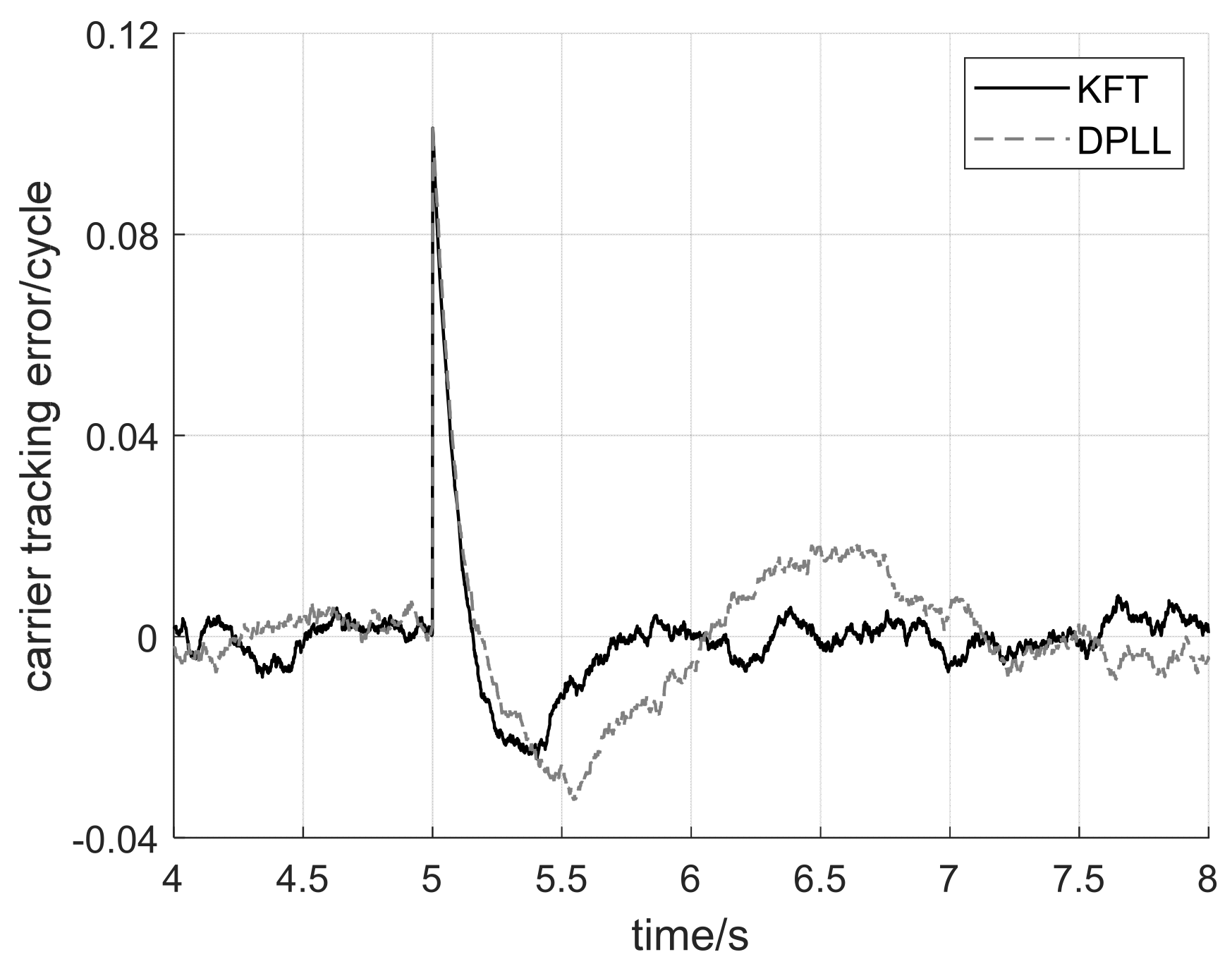
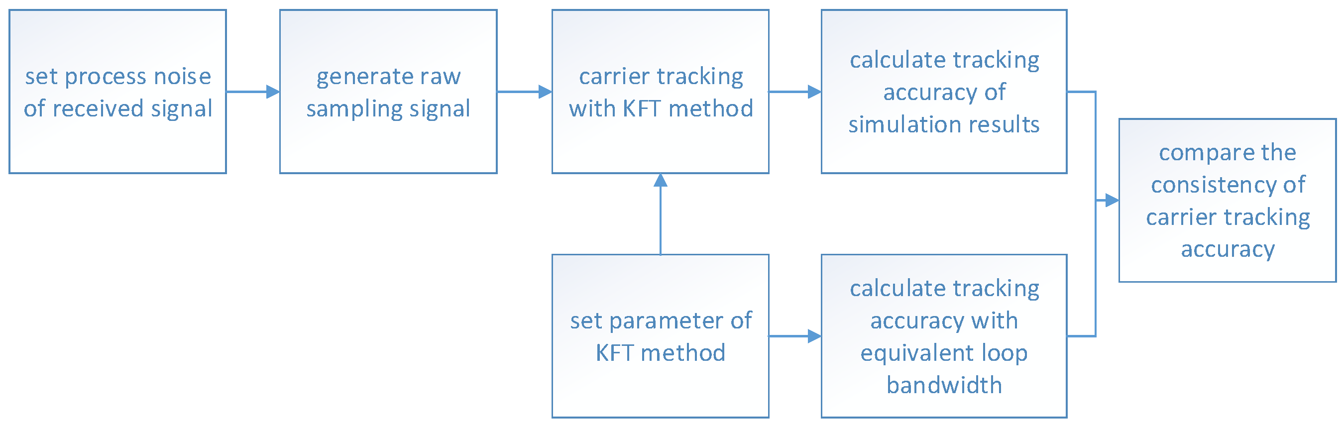
• Implement the KFT method in Figure 1 is for tracking.
• Record the stand deviation of carrier phase error per millisecond as tracking accuracy.
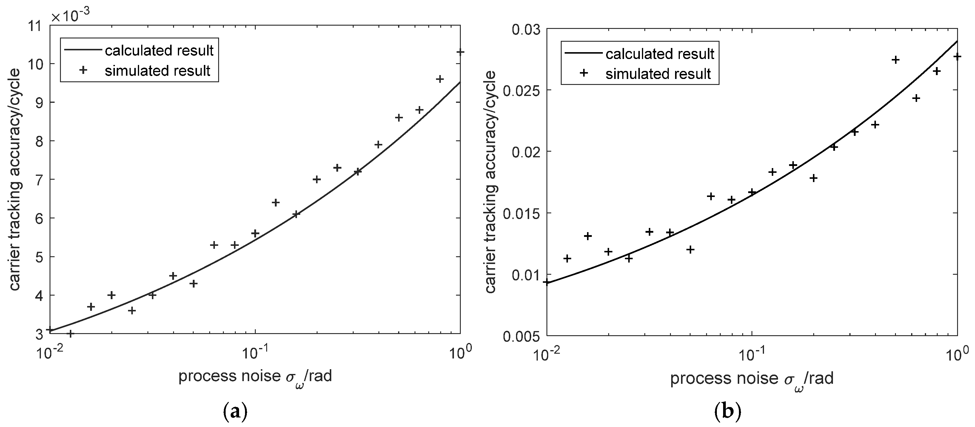
• Calculate equivalent loop bandwidth and tracking accuracy according to (26) and (27).
• Compare simulated and calculated results to validate the analytical expression.

The parameters used in the simulation are shown in

Table 1. Parameters used in simulation.

Parameters	Values
Signal type	BDS B1I
Sampling frequency	10 MHz
Simulation duration	10 s
Carrier-to-noise ratio of received signal	40 dBHz, 30 dBHz
Loop update period	1 ms
Standard deviation of process noise	${10}^{-3}$ rad/Hz
Initial covariance ${\mathbf{P}}_0$	$\left[\begin{array}{cc}100 {\mathrm{r}\mathrm{a}\mathrm{d}}^2& 0\\ 0& 100 {\mathrm{r}\mathrm{a}\mathrm{d}}^2/{\mathrm{s}}^2\end{array}\right]$
Signal length	10 s

:

The simulated and calculated results are shown in Figure 7. To reduce simulation error, 100 independent simulations are carried out, and the mean value for each case is given.

As shown in Figure 7, although slight deviations exist between simulated and calculated results (caused by the thermal noise in signal and more pronounced under low signal-to-noise ratios), the strong consistency validates the correctness of (24) to (26). When the process noise is ${\sigma }_{\omega }=1$ rad, simulations show that the acceleration can exceed 15 g. Figure 2 confirms that KFT simplification does not affect conclusions even under high dynamic conditions.

5. Conclusions

The different parameters of the KFT method and DPLL make performance comparisons challenging. To address this problem, analytical expressions for KFT’s equivalent loop bandwidth are derived by approximating the error feedback model’s innovation. These conclusions enable KFT parameter optimization and accurate performance comparisons between these two fundamentally different techniques.

References

1. Liu, Y.; Zhou, X.X.; Cheng, G.J. High dynamic carrier tracking technology in frequency hopping systems. Syst. Eng. Electron. 2022, 44, 677–683. [Google Scholar]
2. Feng, X.; Zhang, T.S.; Niu, X.; Pany, T.; Liu, J. Improving GNSS carrier phase tracking using a long coherent integration architecture. GPS Solut. 2023, 27, 37. [Google Scholar] [CrossRef]
3. Cui, S.Q.; An, J.P.; Wang, A.H. Kalman filter used for carrier tracking algorithm based on matched maneuvering target model. Syst. Eng. Electron. 2014, 36, 376–381. [Google Scholar]
4. Gardner, F.M. Phaselock Techniques; People’s Posts and Telecommunications Press: Beijing, China, 2007. [Google Scholar]
5. Kay, S.M. Fundamentals of Statistical Signal Processing; Electronic Industry Press: Beijing, China, 2023. [Google Scholar]
6. Cheng, Y.; Chang, Q. A Coarse-to-Fine Adaptive Kalman Filter for Weak GNSS Signals Carrier Tracking. IEEE Commun. Lett. 2019, 23, 2348–2352. [Google Scholar] [CrossRef]
7. Xu, J.W.; Yang, R.; Tang, Z.P.; Zhan, X.; Morton, Y.J. Deeply-Coupled GNSS Dual-Band Collaborative Tracking Using the Extended Strobe Correlator. IEEE Trans. Aerosp. Electron. Syst. 2023, 59, 6164–6178. [Google Scholar] [CrossRef]
8. Cheng, Y.; Zhang, S.K.; Wang, X.Y.; Wang, H.; Yang, H. Kalman Filter with Adaptive Covariance Estimation for Carrier Tracking Under Weak Signals and Dynamic Conditions. Electronics 2024, 13, 1288. [Google Scholar] [CrossRef]
9. Yu, X.Y.; Gao, T.; Sun, G.F.; Tang, X.; Ni, S. Weak GNSS signal tracking algorithm based on variable dimension Kalman filter. J. Natl. Univ. Def. Technol. 2015, 37, 56–60. [Google Scholar]
10. Gómez, M.; Solera-Rico, A.; Valero, E.; Lázaro, J.A.; Fernández-Prades, C. Enhancing GNSS Receiver Performance with Software-Defined Vector Carrier Tracking for Rocket Launching. Results Eng. 2023, 19, 101310. [Google Scholar] [CrossRef]
11. Shen, F.; He, R.; Lv, D.; Zhou, Y. Kalman Filter Based High Dynamic GPS Carrier Tracking Loop. J. Astronaut. 2012, 8, 1041–1047. [Google Scholar]
12. Wang, X.Y.; Chen, X.Y. Strong tracking Kalman filter loop applied for high dynamic GPS signals. J. Southeast Univ. (Nat. Sci. Ed.) 2014, 44, 946–951. [Google Scholar]
13. Sun, P.Y.; Tang, X.M.; Huang, Y.B.; Sun, G. Wavelet de-noising Kalman filter-based Global Navigation Satellite System carrier tracking in the presence of ionospheric scintillation. IET Radar Sonar Navig. 2017, 11, 226–234. [Google Scholar] [CrossRef]
14. Melania, S.; Andreotti, M.; Aquino, M.; Dodson, A. Tuning a Kalman filter carrier tracking algorithm in the presence of ionospheric scintillation. GPS Solut. 2017, 21, 1149–1160. [Google Scholar]
15. Locubiche-Serra, S.; Seco-Granados, G.; López-Salcedo, J.A. Performance assessment of a low-complexity autoregressive Kalman filter for GNSS carrier tracking using real scintillation time series. GPS Solut. 2022, 26, 17. [Google Scholar] [CrossRef]
16. Zhao, W.X.; Khanafseh, S.; Pervan, B. Adaptive Multiple-Model Kalman Filter for GNSS Carrier Phase and Frequency Estimation Through Wideband Interference. J. Inst. Navig. 2024, 71, 646. [Google Scholar] [CrossRef]
17. Hu, Y.; Wu, L.J.; Lou, N.Y.; Liu, W. A Robust Vector-Tracking Loop Based on KF and RTS Smoothing for Shipborne Navigation. J. Mar. Sci. Eng. 2024, 12, 747. [Google Scholar] [CrossRef]
18. Gao, N.; Chen, X.Y.; Yan, Z.; Jiao, Z. Performance Enhancement and Evaluation of a Vector Tracking Receiver Using Adaptive Tracking Loops. Remote Sens. 2024, 16, 1836. [Google Scholar] [CrossRef]
19. Sayed, P.T.; Danilo, P.M. A quaternion frequency estimator for three-phase power systems. In Proceedings of the 2015 IEEE International Conference on Acoustics, Speech and Signal Processing (ICASSP), South Brisbane, Australia, 19–24 April 2015. [Google Scholar]
20. Tang, M.; Cai, S.; Lau, V.K.N. Remote State Estimation with Asynchronous Mission-Critical IoT Sensors. IEEE J. Sel. Areas Commun. 2020, 99, 835–850. [Google Scholar] [CrossRef]
21. Gabr, K.; Abdelkader, M.; Jarraya, I.; AlMusalami, A.; Koubaa, A. SMART-TRACK: A Novel Kalman Filter-Guided Sensor Fusion for Robust UAV Object Tracking in Dynamic Environments. IEEE Sens. J. 2025, 25, 3086–3097. [Google Scholar]
22. Xu, D.; Wang, B.; Zhang, L.; Chen, Z. A New Adaptive High-Degree Unscented Kalman Filter with Unknown Process Noise. Electronics 2022, 11, 1863. [Google Scholar] [CrossRef]
23. Tang, K.H.; Wu, C.F.; Du, L.; He, X. Experimental study and design on high dynamic GNSS receiver using adaptive optimal bandwidth for carrier tracking loop. J. Chin. Inert. Technol. 2014, 12, 498–503. [Google Scholar]
24. Jin, L.; Lv, P.; Cui, X.; Lu, M.; Feng, Z. Adaptive Kalman tracking algorithm for new generation GNSS signals. J. Tsinghua Univ. (Sci. Technol.) 2012, 52, 1249–1254. [Google Scholar]
25. Won, J.; Pany, T.; Eissfeller, B. Characteristics of Kalman filters for GNSS signal tracking loop. IEEE Trans. Aerosp. Electron. Syst. 2012, 48, 3671–3681. [Google Scholar] [CrossRef]
26. Niu, X.J.; Li, B.; Ziedan, N.I.; Guo, W.; Liu, J. Analytical and simulation-based comparison between traditional and Kalman filter-based phase-locked loops. GPS Solut. 2017, 21, 123–135. [Google Scholar] [CrossRef]
27. Bidon, S.; Roche, S. On the equivalence between steady-state Kalman filter and DPLL. Signal Process. 2024, 224, 109591. [Google Scholar] [CrossRef]
28. Qian, Y.; Cui, X.W.; Lu, M.Q. Steady-State Performance of Kalman Filter for DPLL. Tsinghua Sci. Technol. 2009, 14, 470–473. [Google Scholar] [CrossRef]
Figure 1. Implementation block diagram of KFT method.
Electronics 14 02588 g001
Figure 2. Simplified block diagram of KFT method.
Electronics 14 02588 g002
Figure 3. Equivalent loop bandwidth under different observation noise and process noise.
Electronics 14 02588 g003
Figure 4. Damping coefficient corresponding to different process noise.
Electronics 14 02588 g004
Figure 5. Transient response of KFT method and DPLL with loop bandwidth of 3.5 Hz under carrier phase step of 0.1 cycle.
Electronics 14 02588 g005
Figure 6. Simulation process to verify the analytical expression of the equivalent loop bandwidth.
Electronics 14 02588 g006
Figure 7. Simulated and calculated carrier tracking accuracy of KFT method. (a) Carrier-to-noise ratio of 40 dBHz; (b) carrier-to-noise ratio of 30 dBHz.
Electronics 14 02588 g007