YOLO-LSDI: An Enhanced Algorithm for Steel Surface Defect Detection Using a YOLOv11 Network

Abstract

Addressing the difficulties in identifying surface defects in steel and various industrial materials, including challenges in detection, low generalization, and poor robustness, as well as the shortcomings of existing algorithms for industrial applications, this paper presents the YOLO-LSDI algorithm for steel surface defect identification. First, the model integrates the Adaptive Multi-Scale Pooling–Fast (AMSPPF) module, an adaptive multi-scale pooling approach that improves the extraction of global semantic and local edge features. Second, the Deformable Spatial Attention Module (DSAM), a hybrid attention mechanism combining deformable and spatial attention, is introduced to enhance the network’s focus on defect-relevant regions under complex industrial backgrounds. Third, Linear Deformable Convolution (LDConv) replaces standard convolution to better adapt to the irregular shapes of defects while maintaining low computational cost. Finally, the Inner-Complete Intersection over Union (Inner-CIoU) loss function is adopted to improve localization accuracy and training stability. Experimental results on the NEU-DET dataset demonstrate a 5.8% improvement in the mAP@0.5, a 2.4% improvement in the mAP@0.5:0.95, and a 6.2% improvement in the F1-score compared to the YOLOv11n baseline, with GFLOPs reduced to 6.1 and inference speed reaching 162.1 frames per second (FPS). Evaluations on the GC10-DET dataset, APSPC dataset, and a PCB defect dataset further confirm the generalization capability of YOLO-LSDI, with mAP@0.5 improvements of 4.2%, 2.1%, and 3.1%, and corresponding mAP@0.5:0.95 improvements of 1.1%, 1.5%, and 1.3%, respectively. These results validate the effectiveness and practicality of the proposed model for real-time industrial defect-detection tasks.

1. Introduction

With the continuous development and progress of society, steel has found increasingly widespread applications in various fields, including construction, transportation, manufacturing, daily commodities, chemical industries, and pharmaceuticals [1]. As the industrial Internet, big data, and other information technologies continue to advance, intelligent manufacturing is gradually entering a new stage characterized by intelligent processing driven by artificial intelligence [2]. Against this backdrop, quality has become the core of competitiveness in manufacturing industries. In the steel industry in particular, product quality directly impacts the survival and growth of companies. The Made in China 2025 strategy further emphasizes the importance of production quality and promotes the manufacturing sector toward higher standards. Yet, in the production of steel, numerous variables like production methods, the machinery used, and environmental circumstances typically result in surface imperfections, like cracking, inclusions, blotches, pitted surfaces, rolled-in scales, scratches, and more [3]. These flaws impair the product’s appearance, diminish its durability, and may introduce safety concerns. Hence, promptly and correctly identifying and addressing steel surface imperfections is vital for maintaining uninterrupted manufacturing, enhancing product excellence, and reducing safety risks [4].

In traditional manufacturing processes [5], the identification of surface flaws in steel products mainly relies on manual visual evaluation. However, this method has several limitations. First, manual inspection is inefficient and prone to errors due to factors such as fatigue and inattention, making it difficult to ensure accurate detection and often leading to missed or false detections. Moreover, prolonged visual inspection can have adverse effects on workers’ health, and the high labor intensity of manual inspection significantly increases production costs. As a result, manual detection alone can no longer satisfy the requirements of contemporary industrial manufacturing, which requires greater efficiency and precision. As technology advances at a breakneck pace, machine vision-based defect detection systems [6] are slowly but surely becoming integrated into manufacturing processes. These sophisticated systems use high-definition cameras to capture the surface images of products, and then they apply image-processing algorithms to pinpoint any surface flaws with precision. Machine vision [7] technology has significantly improved detection efficiency, reduced human error, and alleviated the workload of workers, thus promoting the automation of the production process.

Traditional image-processing methods [8] generally involve three key steps: preprocessing, feature extraction, and classification. Song et al. [9] proposed a method based on image block percentile color histograms and eigenvector texture features for classification. This approach has proven effective, particularly in detecting defects involving junctions. Ma et al. [10] utilized cosine similarity and color-moment features to verify the periodicity of magneto-optical images, successfully identifying appropriate magneto-optical images for detecting and locating welding defects. Wang et al. [11] developed a Fourier-based image reconstruction technique for magnet surface defect detection. Li et al. [12] combined color-moment features and scale-invariant feature transform (SIFT) features to address the challenge of capturing tile surface defects, which cannot be fully detected using a single feature. Chang et al. [13] introduced an automated inspection system for compact camera lenses, incorporating circle Hough transformation, weighted Sobel filtering, and polar transformations, followed by an SVM classifier for precise defect detection. Liu et al. [14] proposed an enhanced multi-block local binary pattern (LBP) algorithm, which combines the simplicity and efficiency of LBP with an adaptive block scaling technique for improved defect recognition. Putri et al. [15] designed a visual inspection system for automated ceramic surface quality control, using fuzzy logic for digital image processing. Gan et al. [16] explored a novel nondestructive testing approach using magnetic-optical imaging and fractal dimension analysis to detect micro-weld defects on high-strength steel surfaces.

In contrast, deep learning [17] has emerged as a powerful tool capable of automatically learning feature representations from images, simplifying feature extraction processes. As a result, deep learning techniques have progressively replaced traditional image-processing methods and are now widely used for tasks such as steel surface defect detection [18]. He et al. [19] proposed a novel defect-detection system that uses a baseline Convolutional Neural Network (CNN) for feature map generation at each stage, followed by a Multilevel Feature Fusion Network (MFN) to merge hierarchical features, thereby incorporating more location details of defects. Damacharla et al. [20] introduced a transfer learning-based U-Net (TLU-Net) framework for steel surface defect detection. Using a U-Net architecture with ResNet and DenseNet encoders, they demonstrated that transfer learning improved defect classification by 5% compared to random initialization. Bhatt et al. [21] proposed a deep learning segmentation-based model for surface anomaly detection, specifically focusing on surface crack detection. Zhao et al. [22] modified the Faster R-CNN architecture by replacing part of the conventional convolutional layers with deformable convolutions, achieving improved performance in complex target detection. Liu et al. [23] enhanced the YOLOv4 algorithm for fabric defect detection by incorporating a new softPool structure, effectively reducing the negative impact of traditional pooling layers and improving detection accuracy. Zhao et al. [24] introduced RDD-YOLO, an advanced YOLOv5 architecture for detecting defects on steel surfaces. Their model uses a Double Feature Pyramid Network (DFPN) to enhance the neck structure, allowing for deeper network layers and improved feature reuse. Yi et al. [25] presented YOLOv7-SiamFF, a defect-detection framework using YOLOv7 as the backbone with three feature reinforcement modules. This framework was validated using a specialized visual dataset for industrial defect detection, demonstrating effective results. Xie et al. [26] proposed LMS-YOLO, a lightweight model based on YOLOv8 for efficient steel surface defect detection. The model uses a multi-scale mixed convolution (LMSMC) module to fuse features at different scales, optimizing both performance and network efficiency. Zou et al. [27] introduced CK-NET, an improved steel defect-detection model based on YOLOv9c, achieving a 13.2% improvement in the mAP over YOLOv9c while maintaining similar model parameters. Ruengrote et al. [28] applied YOLOv10 for defect detection, incorporating architectural improvements like CSPNet and PANet to enhance feature extraction and fusion, as well as a dual-assignment mechanism to boost localization accuracy. Tang et al. [29] proposed the ConTriNet network, which employs a “divide-and-conquer” strategy by designing three parallel flows to separately extract modality-specific and modality-complementary features. By incorporating a Residual Atrous Spatial Pyramid Module (RASPM), the network effectively enlarges the receptive field and integrates multi-scale contextual information, significantly enhancing robustness and detection performance in complex scenarios. Extensive experiments on multiple public RGB-T salient object-detection datasets demonstrated the superior performance of ConTriNet, validating the effectiveness of its architectural design.

Although deep learning-based defect-detection methods have made considerable progress, challenges remain in the context of steel surface inspection. Many existing models struggle with multi-scale defect recognition, have limited ability to focus on critical regions in complex industrial backgrounds, and rely on fixed receptive fields, which hinders their adaptability to irregular defect shapes. Additionally, commonly used IoU-based loss functions often converge slowly and lack localization precision for small or overlapping defects. Moreover, generalization across different datasets and materials remains limited, restricting their applicability in real-world scenarios. To address these issues, this study proposes an improved version of YOLOv11, termed YOLO-LSDI, which enhances accuracy, efficiency, and robustness in industrial defect-detection tasks. The main highlights of this research are summarized as follows:

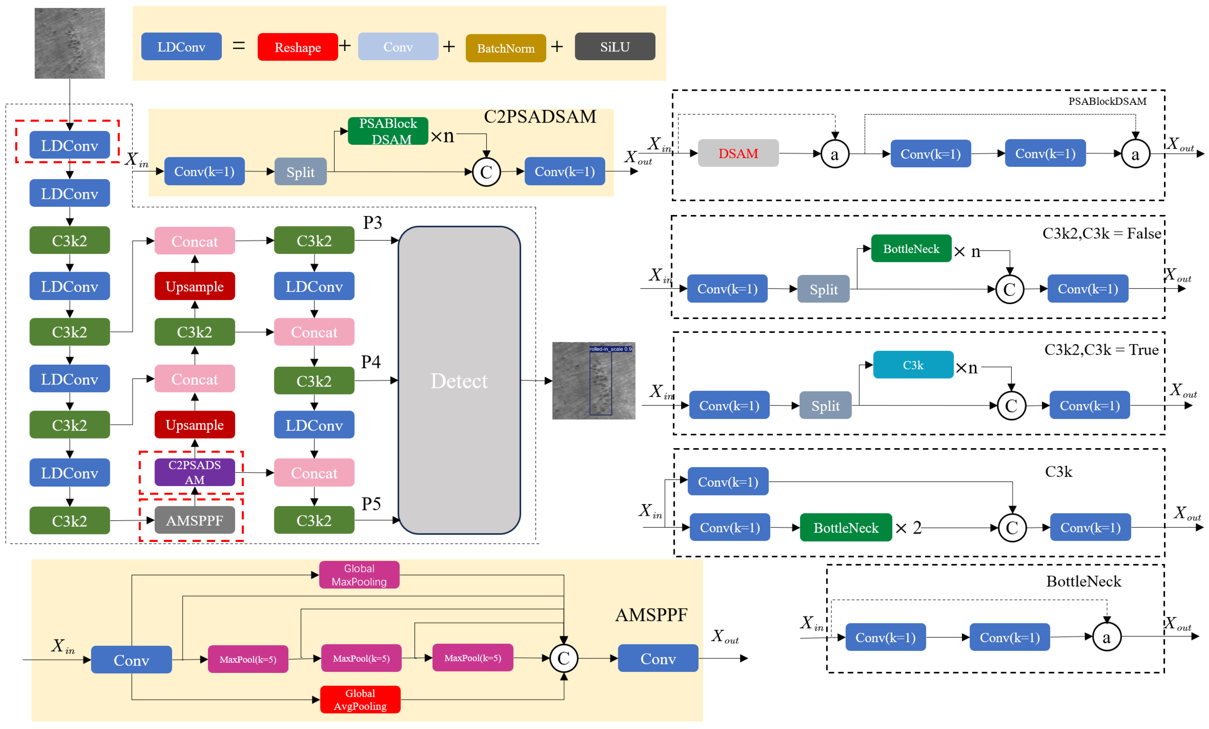
• An Adaptive Multi-Scale Pooling–Fast module (AMSPPF) is introduced to better capture both global semantic context and local edge features by fusing global average pooling (GAP) and global max pooling (GMP). Unlike the original SPPF in YOLOv11, which primarily focuses on fixed-scale local features, AMSPPF provides a broader receptive field and enhanced sensitivity to contour information. This is particularly effective for detecting defects with varying scales and low visual contrast. Experimental results show that AMSPPF contributes to a 2.2% improvement in mAP@0.5 and a 0.8% improvement in mAP@0.5:0.95 on the NEU-DET dataset, along with a 3.8% improvement in the F1-score.
• A Deformable Spatial Attention Module (DSAM) is proposed, combining deformable bi-level attention with a spatial attention mechanism. This hybrid design allows the network to dynamically focus on defect-relevant regions while preserving spatial detail. This proves especially beneficial for fine-grained discrimination of visually similar defect types and in mitigating interference from complex backgrounds—challenges often encountered in steel surface inspection. Integrated into the backbone alongside the C2PSA module, DSAM leads to a further 0.4% improvement in mAP@0.5, a further 0.1% improvement in mAP@0.5:0.95, and a further 0.2% improvement in the F1-score, validating its effectiveness in enhancing feature expressiveness.
• We introduce Linear Deformable Convolution (LDConv) to replace the standard convolutional layers in YOLOv11. Unlike fixed receptive fields, LDConv learns spatial offsets to adapt to the irregular shapes of steel defects, enhancing localization and classification. Moreover, LDConv maintains efficiency through a lightweight design, reducing computational cost. GFLOPs dropped from 6.4 to 6.1, while mAP@0.5 increased by an additional 2.0%, mAP@0.5:0.95 improved by 0.7%, and the F1-score rose 1.0%, achieving higher accuracy without compromising real-time performance.
• We replace the traditional Complete-IoU (CIoU) loss function with the Inner-CIoU, a refined variant that incorporates a scaling factor to regulate the auxiliary box in IoU computation. This design addresses issues such as slow convergence and suboptimal localization accuracy, especially critical when detecting overlapping or small-scale defects under cluttered industrial backgrounds. The proposed loss function accelerates training and stabilizes regression performance, contributing an additional 1.2% improvement in mAP@0.5, a further 0.8% improvement in mAP@0.5:0.95, and a 1.2% improvement in the F1-score while also boosting inference speed to 162.1 FPS. Cumulatively, these enhancements yield a total mAP@0.5 improvement of 5.8% and an mAP@0.5:0.95 improvement of 2.4%, demonstrating the robustness of the proposed framework.
• We validate the generalization ability of our model across multiple industrial defect datasets, including NEU-DET (steel), GC-DET (steel), APSPC (aluminum), and a PCB surface defect dataset. Experimental results indicate consistent and superior performance across domains, with mAP@0.5 improvements of 4.2, 2.1, and 3.1%, respectively, mAP@0.5:0.95 improvements of 1.1, 1.5, and 1.3%, and F1-score improvements of 4.2, 3.3, and 1.5% compared to existing state-of-the-art methods. These findings underline the practical value and deployment potential of the proposed system in diverse real-world inspection scenarios.

The remaining sections of this paper are structured as follows. Section 2 provides a thorough review of the datasets, theoretical frameworks, and methodologies employed throughout this study. In Section 3, we offer an in-depth assessment of the YOLO-LSDI model, highlighting results from a variety of comparison tests and ablation studies. Moving on, Section 4 explores the major insights gained and the limitations encountered in this research. To wrap things up, Section 5 provides a concise summary of the key contributions made by this work.

2. Materials and Methods

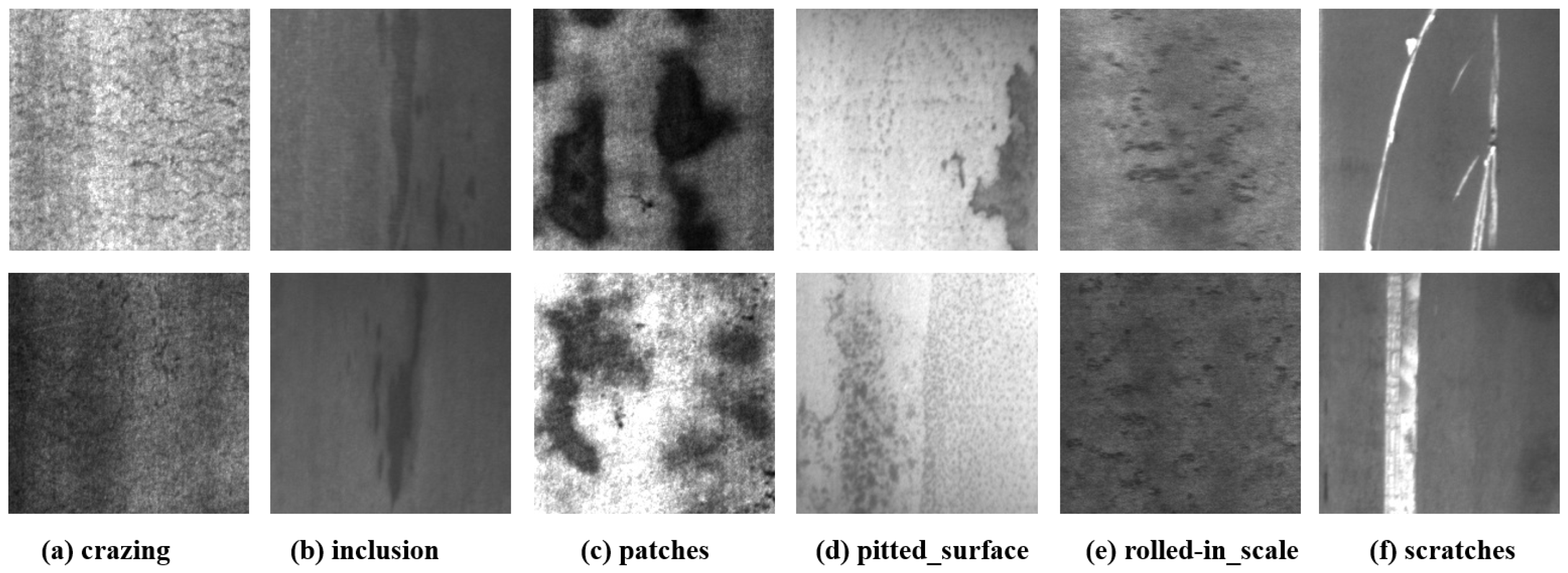
2.1. Experimental Dataset

2.1.1. Dataset Source

The steel manufacturing industry is no stranger to challenges, particularly when it comes to the intricate production methods and demanding conditions that often lead to a variety of surface imperfections. For this research, we mainly focus on the steel strip surface defect dataset (NEU-DET) provided by Song’s team at Northeastern University (NEU) [19,30]. This comprehensive dataset encompasses six prevalent defect categories: crazing, inclusions, patches, pitted surfaces, rolled-in scales, and scratches. Each category is represented by 300 grayscale images, each standardized to a resolution of 200 × 200 pixels. Figure 1 showcases a selection of representative images highlighting these six defect types.

The six defect types exhibit distinct features and formation mechanisms. Crazing appears as transverse or longitudinal cracks, typically caused by internal defects or thermal stress from temperature changes. Inclusions involve irregular, protruding particles formed by impurities or non-metallic materials mixed into the steel during production. Patches are large, uneven surface areas resulting from internal inhomogeneity and uneven rolling or cooling. Pitted surfaces feature small, dot-like depressions, usually caused by oxidation or corrosion. Rolled-in scales show fish scale- or block-like oxidized layers in red-black tones, formed when hot steel reacts with oxygen. Scratches are linear marks caused by contact with hard objects during processing, storage, or transportation.

2.1.2. Dataset Analysis

As shown in Figure 1, defects within the same category in the NEU dataset vary significantly in appearance. For instance, scratches can appear as horizontal, vertical, or inclined marks. Lighting conditions and material properties also cause noticeable grayscale differences within the same defect type. Furthermore, different categories may share similar morphological features—for example, crazing, rolled-in scales, and pitted surfaces often look alike. Statistical analysis revealed an uneven distribution of defect types, with these visually similar categories being relatively rare, as illustrated in the left part of Figure 2. In addition, many defects have low contrast against the background, resulting in blurred edges and feature fusion, which makes them difficult to distinguish. Additionally, many defects exhibit low contrast with the background, leading to a high degree of fusion between the defect features and the background, which results in blurred edges that make the defects difficult to identify.

Besides the visual characteristics of the images, defect size is also a critical factor in the dataset. Variations in defect scale provide valuable guidance for model design. To explore this, we analyzed the area ratio of each defect region, as shown in the right part of Figure 2. The NEU dataset includes a wide range of defect sizes, from tiny marks with minimal area coverage to large defects occupying almost the entire image. Notably, small defects with an area ratio below 10% account for 44.94% of all cases, while those between 0 and 20% represent over 70% of the total. This indicates that small-sized defects are dominant; thus, our study focuses on fine-grained defects that are more easily affected by the background.

In summary, based on the statistical analysis of the steel surface defect dataset, the main focus of the study is established: to improve existing models to overcome challenges such as variations within the same defect category, morphological similarities between different categories, high fusion of defects with the background, and detection difficulties caused by differences in defect size. These challenges result in poor generalization ability and robustness in current models. Moreover, the models must remain lightweight, with low computational complexity.

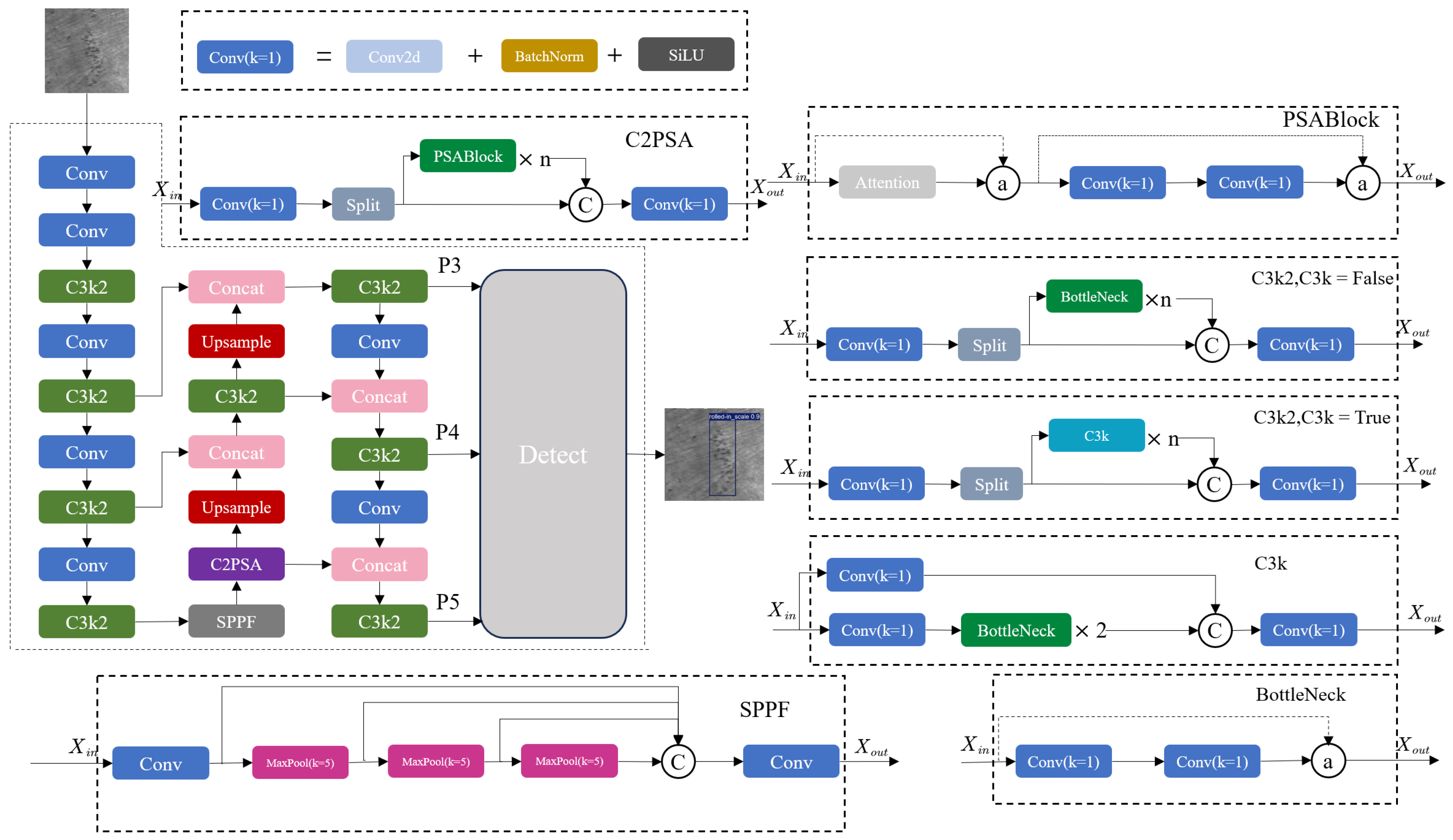
2.2. YOLOv11 Algorithm

YOLOv11 [31] is the newest release from the Ultralytics team, demonstrating superior results in detection, segmentation, pose estimation, tracking, and classification. This model incorporates a more efficient architecture and optimized training procedures, achieving improved processing speed while maintaining high accuracy. The YOLOv11 network structure is shown in Figure 3.

YOLOv11 enhances feature extraction by redesigning the backbone and neck networks, introducing modules such as Cross-Stage Partial with kernel size 2 (C3k2) and a Convolutional block with Parallel Spatial Attention (C2PSA). C3k2, derived from the C2f module in YOLOv8 [32], offers flexible configuration by allowing the selection between C3k and bottleneck via a Boolean parameter. C2PSA, inspired by the PSA module in YOLOv10 [33], includes both C2PSA and C2fPSA variants. In practice, the C2-based C2PSA was chosen for implementation. These architectural innovations significantly improve YOLOv11’s performance in complex scenarios such as multi-object detection and occlusion handling. Since feature extraction plays a critical role in object localization and classification, the enhancements in YOLOv11 lead to higher detection sensitivity and accuracy. Moreover, YOLOv11 integrates two Depthwise Convolution (DWConv) blocks [34] into the classification head of the original decoupled head. This significantly reduces computational cost while maintaining—or even improving—detection performance. Such efficiency gains are especially valuable in resource-constrained settings, including edge devices and low-power embedded systems.

A key difference between YOLOv11 and YOLOv8 lies in how they scale network depth and width across model variants (N, S, M, L, and X). In YOLOv11, the depth multiplier adjusts the number of layers, while the width multiplier controls the number of channels per layer. Lightweight versions (e.g., YOLOv11-N) use smaller scaling factors to reduce parameters and computational cost, making them suitable for real-time or resource-limited scenarios. Larger variants (e.g., YOLOv11-L and YOLOv11-X) increase both depth and width to improve feature representation and learning capacity. This flexible scaling balances efficiency and accuracy, compensating for smaller model sizes by restoring capacity where needed. On the COCO dataset [35], YOLOv11n has achieved a remarkable balance between low parameter count and computational complexity, with only 6.5 billion operations. For steel defect detection—often constrained by computational resources—a lightweight yet effective model is essential for accuracy improvement.

Therefore, this study adopts YOLOv11n as the baseline, optimizing its components to meet industrial defect-detection needs. Its low computational cost and streamlined architecture provide a strong foundation for enhancing the detection of fine-grained, low-contrast, and irregular defects commonly found on steel surfaces in complex industrial environments.

2.3. YOLO-LSDI Algorithm

The improved network structure is shown in Figure 4. First, the Adaptive Multi-Scale Pooling–Fast (AMSPPF) module is introduced to capture broader contextual information while reducing the impact of scale variations in defect patterns. Second, the Deformable Spatial Attention Module (DSAM) enhances the network’s focus on defect-relevant regions, improving feature extraction. Third, the standard convolution in YOLOv11 is replaced with Linear Deformable Convolution (LDConv), addressing fixed receptive field limitations and boosting both accuracy and computational efficiency. Finally, the original Complete-IoU (CIoU) loss is replaced with the Inner-CIoU, which improves generalization and localization, especially for small or overlapping defects. Together, these enhancements enable the proposed model to balance detection precision, inference efficiency, and robustness across diverse industrial inspection tasks.

2.3.1. A New Spatial Pyramid Module: AMSPPF

The Spatial Pyramid Pooling (SPP) module, originally proposed by He et al. [36], addresses two key issues. First, it reduces the extraction of redundant features in Convolutional Neural Networks (CNNs), significantly accelerating the generation of candidate bounding boxes and lowering computational costs. Second, it avoids the image distortion typically introduced by cropping and resizing, enabling the network to process input images of arbitrary sizes and aspect ratios.

SPP applies max pooling using three kernels of different sizes on each feature map, producing pooled outputs of predefined dimensions. These outputs are then flattened and concatenated into a single feature vector, as illustrated in Figure 5a. In contrast, the Spatial Pyramid Pooling–Fast (SPPF) module [37] replaces the original multi-scale pooling with three consecutive 5 × 5 max-pooling layers. This modification retains similar accuracy while reducing computational complexity. By leveraging fixed-size pooling, SPPF improves feature extraction efficiency and enhances recognition performance. The structure is shown in Figure 5b.

To better tackle the challenges of steel surface defect detection, we extend the SPPF module by integrating global average pooling and global max pooling, followed by feature concatenation, as shown in Figure 5c. The resulting module, named Adaptive Multi-Scale Pooling–Fast (AMSPPF), enriches the original SPPF module by capturing more comprehensive global context and enhancing spatial feature diversity. While SPPF primarily emphasizes edge information, it often neglects broader background features, limiting its effectiveness in detecting subtle textures or scale-varying defects, especially in complex industrial settings. By incorporating diverse pooling strategies, AMSPPF improves the model’s ability to recognize defect patterns under a wide range of visual conditions.

2.3.2. New Module Based on C2PSA: C2PSA-DSAM

Although YOLOv11 shows significant improvements over previous models, the proposed C2PSA module does not perform as expected. Despite incorporating a multi-head attention mechanism, the module places less emphasis on both channel and spatial attention, which negatively affects fine-grained feature extraction. For instance, defects in steel, such as two specific types, are highly susceptible to complex backgrounds and varying scales. This limitation motivated us to seek improvements by introducing a more efficient and lightweight attention mechanism to enhance the feature extraction capabilities of the module.

The Convolutional Block Attention Module (CBAM) [38] is a lightweight attention module that combines both channel and spatial attention mechanisms to enhance the network’s representational power. As shown in Figure 6 (above), the CBAM consists of two submodules: a Channel Attention Module (CAM) and a Spatial Attention Module (SAM), which apply attention at the channel and spatial levels, respectively. The CBAM is relatively easy to integrate into existing network structures and can improve model performance. However, the need to compute both channel and spatial attention increases computational complexity, which may impact the model’s expressiveness and generalization ability.

To enhance global context modeling while maintaining computational efficiency, we integrate the Deformable Bi-level Routing Attention (DBRA) module [39] into our framework. DBRA is a two-stage attention mechanism that enables the model to focus on both coarse global structure and fine-grained spatial details—an essential capability for detecting irregular and small-scale defects on steel surfaces. In the coarse routing stage, the input feature map $X\in {\mathrm{R}}^{H\times W\times C}$ is divided into N non-overlapping spatial regions. For each query region $r_q$, a coarse attention score is computed over key regions $r_k$ as

$${\alpha }_{qk}=\mathrm{Softmax}\left({\displaystyle \frac{Q_{r_q}{K}_{r_k}^{\top }}{\sqrt{d}}}\right)$$

(1)

In the fine-grained deformable attention stage, attention is restricted to the top-k most relevant regions as determined by the routing stage. For each selected region, a set of deformable sampling offsets $\mathsf{\Delta }{p}_i$ is learned, enabling the model to capture irregular defect patterns. The attention output is computed as

$$\mathrm{Attn}\left(x_q\right)=\sum _{i=1}^M{w}_i·x(p_q+\mathsf{\Delta }{p}_i)$$

(2)

where $x(p_q+\mathsf{\Delta }{p}_i)$ denotes the bilinearly interpolated feature at the sampled location and $w_i$ are learnable attention weights. This bi-level strategy significantly reduces computational complexity from $\mathcal{O}{\left(HW\right)}^2$ in full attention to $\mathcal{O}(N^2+NM)$ while improving spatial adaptability—a crucial property in steel surface defect detection, where defects often exhibit irregular morphology and scattered distribution.

DBRA improves the selection of key–value pairs through proxy queries, producing more accurate and interpretable attention maps. This is particularly useful for detecting subtle surface anomalies that are easily affected by texture noise or scale variation. By combining DBRA with the SAM, we designed a new attention module—the Deformable Bi-level Spatial Attention Module (DSAM)—as shown in Figure 6. In this structure, DBRA captures long-range dependencies via deformable region-based attention, enabling adaptation to varying defect shapes and scales. Meanwhile, the SAM emphasizes spatially informative regions by aggregating channel-wise responses. We embed the DSAM into the C2PSA framework, forming the enhanced C2PSA-DSAM. Experiments show that this module significantly improves the network’s ability to detect small and ambiguous defects, enhancing robustness on complex steel surface datasets. The module’s architecture is shown in Figure 7.

2.3.3. Introducing LDConv

Linear Deformable Convolution (LDConv) [40] is introduced to overcome the limitations of standard convolution. Standard convolution operates within a fixed-size, rigid local window, which makes it challenging to dynamically adapt to the varying shapes of different objects. While Deformable Convolution enables flexible sampling positions, its parameters grow quadratically with the kernel size, leading to reduced computational efficiency. In contrast, LDConv provides greater flexibility by allowing the parameters of the convolution kernel to grow linearly, thus mitigating the quadratic growth in parameter count and striking an improved trade-off between network load and efficiency. The process of feature extraction by LDConv can be divided into three steps.

Taking $N=5$ as an example (see Figure 8), the LDConv module operates in three key steps. First, the initial sampling patterns ($P_n$) are generated based on the kernel size N using the initial sampling algorithm and are added to the base coordinates ($P_0$) to obtain the initial sampling positions $(P_0+P_n)$, which define the spatial locations for the convolution kernel. Second, learnable offsets are predicted via a convolutional layer, producing an offset map of shape ($B,2N,H,W$). These offsets are added to the initial coordinates to generate adaptive sampling positions, allowing the kernel to dynamically adjust its sampling shape at each spatial location according to the local content. Finally, the features at the computed sampling positions are extracted through interpolation and resampling, followed by convolution over these features. Through these three steps, LDConv enables convolution operations with arbitrary and adaptive sampling patterns, enhancing the model’s flexibility and feature extraction capability.

LDConv uses a coordinate generation algorithm to produce initial sampling positions for convolution kernels of any size. These positions are dynamically adjusted via learnable offsets, allowing the kernel to better adapt to the shape and scale of local features, thus improving feature extraction efficiency. This adaptive sampling is especially beneficial for steel surface defect detection, where defects often have irregular shapes, varying scales, and low contrast with the background. By replacing standard convolution with LDConv, the network can focus more precisely on defect regions, leading to significant improvements in detection accuracy and computational efficiency.

2.3.4. Inner-CIoU Loss

In the field of object detection, bounding boxes are used to precisely mark the position and size of objects within an image. The accuracy of a model in pinpointing these objects largely depends on the bounding-box regression loss function, which plays a critical role in ensuring accurate localization. Yu et al. [41] revolutionized this aspect by proposing the Intersection over Union (IoU) loss. This innovative approach evaluates the overlap between the predicted bounding box and the actual ground-truth (GT) box by computing the ratio of their intersecting area to their combined area. This improves the model’s grasp of spatial connections during training and boosts its predictive precision. The IoU is mathematically expressed as

$$\mathrm{IoU}={\displaystyle \frac{\left|B\cap B^{\mathrm{gt}}\right|}{\left|B\cup B^{\mathrm{gt}}\right|}}$$

(3)

where B and $B^{\mathrm{gt}}$ represent the predicted and GT boxes, respectively. The corresponding IoU loss is then

$$L_{\mathrm{IoU}}=1-\mathrm{IoU}$$

(4)

Despite its effectiveness, the IoU suffers from some limitations. For example, when the predicted box and the GT box have no overlap, the IoU equals zero, which results in a loss of one. This does not reflect the spatial distance between the boxes, and the loss remains the same even when the predicted box is close to the GT box. Furthermore, if two boxes have the same IoU but different positions, the IoU loss cannot distinguish which box is more accurate. To address these issues, Zheng et al. [42] introduced the Complete IoU (CIoU), which incorporates distance and shape loss components, improving the accuracy of box alignment. The CIoU loss function is defined as

$$L_{\mathrm{CIoU}}=1-\mathrm{IoU}+{\displaystyle \frac{{\rho }^2(b,b^{\mathrm{gt}})}{c^2}}+\alpha v$$

(5)

where $\alpha$ is a positive trade-off parameter:

$$\alpha ={\displaystyle \frac{v}{(1-\mathrm{IoU})+v}}$$

(6)

and v measures the aspect ratio consistency:

$$v={\displaystyle \frac{4}{{\pi }^2}}{(arctan{\displaystyle \frac{w^{\mathrm{gt}}}{h^{\mathrm{gt}}}}-arctan{\displaystyle \frac{w}{h}})}^2$$

(7)

where $w^{\mathrm{gt}}$, $h^{\mathrm{gt}}$, w, and h represent the widths and heights of the GT and predicted boxes, respectively.

Although the CIoU offers an improved description of bounding-box regression, it mainly accelerates convergence by adding extra loss components without addressing the IoU’s inherent limitations. In many detection tasks, such as defect detection in steel datasets, the IoU loss struggles due to varying defect shapes and sizes, which reduces its generalization ability. To address this, Zhang et al. [43] proposed the Inner-IoU loss, which introduces a scale factor to generate auxiliary bounding boxes of varying sizes, thereby improving the regression process across different detection contexts.

As illustrated in Figure 9, the ground-truth box is indicated as $B^{\mathrm{gt}}$, while the anchor box is labeled as B. The coordinates for the center points of the ground-truth box and its internal centers are expressed as $(x_c^{\mathrm{gt}},y_c^{\mathrm{gt}})$, whereas the center points for the anchor box and its internal section are noted as $(x_c,y_c)$. The dimensions of the ground-truth box are represented by $w^{\mathrm{gt}}$ for the width and $h^{\mathrm{gt}}$ for the height, in contrast to the anchor box, which is denoted by w for the width and h for the height. The variable “ratio” signifies the scale factor, which generally falls within the range of [0.5, 1.5]. The calculation of the Inner-IoU loss is performed as follows:

$$b_l^{\mathrm{gt}}=x_c^{\mathrm{gt}}-{\displaystyle \frac{w^{\mathrm{gt}}\ast radio}{2}},b_r^{\mathrm{gt}}=x_c^{\mathrm{gt}}+{\displaystyle \frac{w^{\mathrm{gt}}\ast radio}{2}}$$

(8)

$$b_t^{\mathrm{gt}}=y_c^{\mathrm{gt}}-{\displaystyle \frac{w^{\mathrm{gt}}\ast radio}{2}},b_b^{\mathrm{gt}}=y_c^{\mathrm{gt}}+{\displaystyle \frac{w^{\mathrm{gt}}\ast radio}{2}}$$

(9)

$$b_l=x_c-{\displaystyle \frac{w\ast radio}{2}},b_r=x_c+{\displaystyle \frac{w\ast radio}{2}}$$

(10)

$$b_t=y_c-{\displaystyle \frac{w\ast radio}{2}},b_b=y_c+{\displaystyle \frac{w\ast radio}{2}}$$

(11)

$$inter=(min(b_r^{\mathrm{gt}},b_r)-max(b_l^{\mathrm{gt}},b_l)\ast (min(b_b^{\mathrm{gt}},b_b)-max(b_t^{\mathrm{gt}},b_t))$$

(12)

$$union=(w^{\mathrm{gt}}\ast h^{\mathrm{gt}})\ast {\left(ratio\right)}^2+(w\ast h)\ast {\left(ratio\right)}^2-inter$$

(13)

$${\mathrm{IoU}}^{\mathrm{inner}}={\displaystyle \frac{inter}{union}}$$

(14)

The Inner-IoU loss extends the IoU loss by incorporating a scale factor, allowing for more efficient bounding-box regression. When the ratio is less than 1, the auxiliary box is smaller, accelerating convergence for high IoU samples. Conversely, a larger ratio helps with low IoU samples by expanding the regression range.

The modified loss functions using the Inner-IoU are as follows:

$$L_{Inner\text{-}\mathrm{IoU}}=1-{\mathrm{IoU}}^{inner}$$

(15)

$$L_{Inner\text{-}\mathrm{GIoU}}=L_{\mathrm{GIoU}}+\mathrm{IoU}-{\mathrm{IoU}}^{Inner}$$

(16)

$$L_{Inner\text{-}\mathrm{DIoU}}=L_{\mathrm{DIoU}}+\mathrm{IoU}-{\mathrm{IoU}}^{Inner}$$

(17)

$$L_{Inner\text{-}\mathrm{CIoU}}=L_{\mathrm{CIoU}}+\mathrm{IoU}-{\mathrm{IoU}}^{Inner}$$

(18)

In this study, the Inner-CIoU loss replaces the traditional CIoU loss within the YOLOv11 framework. By introducing a scaling factor to refine auxiliary bounding-box dimensions, the Inner-CIoU enhances bounding-box regression accuracy and addresses the CIoU’s limited generalization across varying object shapes and sizes. This improvement is particularly valuable for steel surface defect detection, where defects tend to be small, irregular, and low-contrast. Accurate localization of such defects demands precise and robust bounding-box regression. Experimental results confirm that the Inner-CIoU loss significantly boosts detection performance on steel surface defect datasets, demonstrating its effectiveness in complex industrial scenarios.

3. Results

3.1. Experimental Setup and Training Parameters

The study was carried out on a 64-bit Ubuntu 20.04.6 LTS system, equipped with 128 GB of RAM and an NVIDIA GeForce RTX 3090 GPU. To speed up processing, we employed Python 3.9.7 with PyTorch 1.10.0 as our deep learning toolkit and made use of CUDA 11.4 for hardware acceleration.

The NEU-DET dataset, as outlined in Section 2 , was used as the foundation for the experiments, with input images standardized to a resolution of 640 × 640. The dataset consists of 1800 images, which were divided into training, validation, and test sets at a ratio of 7:2:1, resulting in 1260 training images, 360 validation images, and 180 test images. To enhance the diversity of the training data, the mosaic technique was employed for data augmentation. The training process began with an initial learning rate of 0.01 and a batch size of 64, running for a total of 500 epochs. Unless otherwise specified, all hyperparameters were kept at their default settings. Additionally, the random seed was set to the default value of 0 to ensure consistent experimental conditions. These configurations were uniformly applied across all experiments conducted in this study.

3.2. Evaluation Metrics

The evaluation metrics in this study include mAP@0.5, map@0.5:0.95, F1-score, GFLOPs, parameters (params), and frames per second (FPS).

Precision (P) indicates the proportion of correct positive predictions among all instances the model has labeled as positive. Conversely, recall (R) gauges how many of the actual positive cases the model has successfully detected, expressed as the ratio of true positives to the total number of real positives. The formulas for computing precision and recall are as follows:

$$\mathrm{P}={\displaystyle \frac{\mathrm{TP}}{\mathrm{TP}+\mathrm{FP}}}$$

(19)

$$\mathrm{R}={\displaystyle \frac{\mathrm{TP}}{\mathrm{TP}+\mathrm{FN}}}$$

(20)

In steel surface defect detection, true positives (TP), false positives (FP), and false negatives (FN) correspond to the accurate identification of defects, the erroneous flagging of non-defects, and the oversight of actual defects, respectively. Precision and recall are two pivotal performance indicators in this domain. Typically, these metrics share an inverse correlation: when recall improves, precision often takes a hit, and conversely, as precision rises, recall tends to dip. Striking the right balance between the two is key to optimizing detection systems.

The precision–recall (P-R) curve is a critical tool for assessing a model’s effectiveness, with recall plotted along the horizontal axis and precision along the vertical. The Area Under the Curve (AUC) corresponds to the average precision (AP), a pivotal metric that reflects the model’s detection capabilities. A larger AP value indicates superior performance. The formula for computing AP is as follows:

$$\mathrm{AP}={\displaystyle \frac{1}{\mathrm{N}}}\sum _{\mathrm{i}=1}^{\mathrm{N}}\mathrm{p}\left({\mathrm{r}}_{\mathrm{i}}\right)$$

(21)

In the formula, N represents the number of samples, $\mathrm{p}\left({\mathrm{r}}_{\mathrm{i}}\right)$ denotes the evenly spaced values of recall, and the precision at the i-th recall value is represented by the corresponding accuracy.

Average precision (AP) evaluates the precision for a specific class, whereas the mean average precision (mAP) takes the average of AP scores across all classes within a dataset. This metric serves as a comprehensive indicator of an algorithm’s effectiveness across the entire dataset. The calculation process is outlined as follows:

$$\mathrm{mAP}={\displaystyle \frac{1}{\mathrm{K}}}\sum _{\mathrm{i}=1}^{\mathrm{K}}\mathrm{AP}\left(\mathrm{j}\right)$$

(22)

In the formula, AP represents the average precision for the j-th class, and K denotes the total number of classes.

The mAP@0.5 metric denotes the mean average precision calculated at an IoU threshold of 0.5. In practical terms, a detection is considered correct if the predicted bounding box overlaps with the ground truth by at least 50%. This metric is widely used in object-detection tasks and serves as a reliable indicator of a model’s ability to localize targets accurately. In addition to mAP@0.5, this study also reports mAP@0.5:0.95, which represents the average mAP calculated across multiple IoU thresholds ranging from 0.5 to 0.95 in steps of 0.05. This stricter and more comprehensive metric enables a holistic assessment of the model’s detection performance under varying localization precision requirements.

The F1-score is the harmonic mean of precision (P) and recall (R), providing a balanced evaluation of a model’s detection capability. It is particularly valuable in scenarios with class imbalance or when both false positives and false negatives need to be carefully controlled. The F1-score is calculated as

$$\mathrm{F}1\text{-}\mathrm{score}=2\times {\displaystyle \frac{\mathrm{Precision}\times \mathrm{Recall}}{\mathrm{Precision}+\mathrm{Recall}}}$$

(23)

This metric emphasizes the trade-off between P and R, offering a single value that reflects the overall detection effectiveness. In the context of steel surface defect detection, the F1-score serves as a reliable indicator of a model’s ability to accurately identify defect regions while avoiding unnecessary false alarms.

A confusion matrix is a performance evaluation tool for classification models that summarizes the relationship between the predicted and actual class labels. Each row of the matrix corresponds to the true class, while each column corresponds to the predicted class. The confusion matrix facilitates the calculation of key metrics such as accuracy, precision, recall, and F1-score, enabling a comprehensive assessment of a model’s classification performance.

GFLOPs, or Giga Floating-Point Operations per Second, quantifies the sheer volume of floating-point calculations a model can execute within a single second. This metric serves as a benchmark for assessing the computational intensity and intricacy of the model. Params, short for parameters, denote the total count of adjustable elements within the model, offering insights into its overall scale and sophistication. Generally speaking, a model with a higher parameter count tends to be more expansive and intricate. FPS, or frames per second, measures how many images the model can handle in a one-second timeframe. A higher FPS value translates to superior real-time performance, making the model ideal for applications where swift inference is critical. The formula used to calculate these metrics is as follows:

$$\mathrm{FPS}={\displaystyle \frac{\mathrm{frameNum}}{\mathrm{elapsedTime}}}$$

(24)

where frameNum denotes the complete count of processed frames and elapsedTime represents the consumed time.

3.3. Ablation Experiments

To assess and validate the effectiveness of the proposed improvements and to investigate whether there are any conflicts between different improvement strategies, we formulated the following two optimization schemes:

• Single-strategy optimization scheme: This scheme primarily evaluated the impact of using a single strategy to improve the detection performance of the original model.
• Combined-strategy optimization scheme: This scheme primarily evaluated the impact of combining different strategies to optimize the detection performance of the original model.

In this section, we conduct 10 sets of ablation experiments on NEU-DET, and the detailed experimental results are shown in

Table 1. Ablation experiments of the proposed improvements.

Sequence	AMSPPF	C2PSA-DSAM	LDConv	Inner-CIoU	Params	GFLOPs	mAP@0.5	mAP@0.5:0.95	F1	FPS
1	-	-	-	-	2.5	6.4	77.2	45.6	72.1	158.3
2	✓				2.6	6.4	79.4	46.4	75.9	163.9
3		✓			2.8	6.4	78.8	45.8	74.1	171.2
4			✓		2.4	6.0	80.5	46.9	75.9	150.8
5				✓	2.5	6.4	78.9	46.1	73.8	195.1
6	✓	✓	✓		2.7	6.1	81.8	47.2	77.1	135.6
7	✓	✓		✓	2.9	6.4	79.8	46.5	76.1	207.3
8	✓		✓	✓	2.4	6.1	81.1	47.0	76.8	142.8
9		✓	✓	✓	2.7	6.1	80.8	46.6	76.2	157.2
10	✓	✓	✓	✓	2.7	6.1	83.0	48.0	78.3	162.1

.

In the first five ablation groups (Sequences 1–5), we assessed the impact of each component individually on detection performance. The baseline YOLOv11n model (Sequence 1) achieved an mAP@0.5 of 77.2%, mAP@0.5:0.95 of 45.6%, and F1-score of 72.1%, serving as the reference. Introducing the AMSPPF module (Sequence 2) increased the mAP@0.5 to 79.4% and the F1-score to 75.9%, highlighting its ability to aggregate global semantic and local edge features, which are critical for detecting scale-variant and low-contrast defects. Sequence 3 added the C2PSA-DSAM, combining bi-level routing and spatial attention to better focus on salient defect regions. This resulted in an mAP@0.5 of 78.8% and improved precision with stable recall, demonstrating enhanced discrimination of visually similar defects and reduced background noise. Replacing the conventional convolution with LDConv in Sequence 4 boosted the mAP@0.5 to 80.5% and maintained the F1-score at 75.9% while lowering GFLOPs from 6.4 to 6.0. This confirmed LDConv’s flexible modeling of irregular defect shapes and its computational efficiency. Finally, Sequence 5 employed the Inner-CIoU loss to refine bounding-box regression for small or overlapping defects, achieving an mAP@0.5 of 78.9% and an F1-score of 73.8%, indicating improved localization and training stability. Overall, these results show that each module contributes unique benefits to detection accuracy, generalization, and efficiency, providing a solid foundation for their combined use.

Groups 6–10 represent combined-strategy optimization schemes. For clarity, we label AMSPPF, C2PSA-DSAM, LDConv, and Inner-CIoU as modules 1, 2, 3, and 4, respectively. These combinations address key challenges in steel surface defect detection, including multi-scale variability, complex backgrounds, irregular defect shapes, and localization accuracy, by integrating complementary modules.

Group 6 combined modules 1, 2, and 3, significantly improving detection precision and localization robustness. It achieved an mAP@0.5 of 81.8%, mAP@0.5:0.95 of 47.2%, F1-score of 77.1%, and reduced GFLOPs to 6.1. The synergy of AMSPPF’s global–local semantic fusion, C2PSA-DSAM’s spatially adaptive attention, and LDConv’s deformable representation enabled the effective capture of structural variations and defect morphology. Notably, the combined performance exceeded the sum of individual gains, confirming their strong complementarity. Group 7 integrated modules 1, 2, and 4, focusing on attention mechanisms and regression optimization. This setup achieved the highest inference speed (207.3 FPS) with competitive accuracy—an mAP@0.5 of 79.8%, mAP@0.5:0.95 of 46.5%, and F1-score of 76.1%. However, the absence of LDConv reduced its adaptability to irregular shapes, indicating that the Inner-CIoU’s localization improvements cannot fully replace spatial deformability, highlighting the need for functional complementarity. Group 8 used modules 1, 3, and 4, forming a compact, high-performing model with an mAP@0.5 of 81.1%, an mAP@0.5:0.95 of 47.0%, an F1-score of 76.8%, and the lowest parameter count (2.4 million). AMSPPF and LDConv provide implicit attention and spatial adaptability, while the Inner-CIoU loss refines localization, achieving efficient synergy that balances complexity and performance. Group 9 combined modules 2, 3, and 4, yielding an mAP@0.5 of 80.8%, an mAP@0.5:0.95 of 46.6%, an F1-score of 76.2%, and GFLOPs of 6.1. This combination excelled at suppressing background noise and refining object boundaries. However, the absence of AMSPPF weakened multi-scale defect handling, emphasizing the importance of global semantic context modeling. Group 10 integrated all four modules, forming the complete YOLO-LSDI framework and achieving the best overall performance: an mAP@0.5 of 83.0%, an mAP@0.5:0.95 of 48.0%, an F1-score of 78.3%, and a balanced FPS of 162.1. These improvements did not increase the GFLOPs or parameters beyond those of Groups 6 or 9, proving that each module offers distinct, non-overlapping benefits. The full integration achieved synergistic optimization, balancing accuracy, speed, and generalization to meet real-time industrial inspection demands.

3.4. Attention Heatmap Visualization of Module Improvements

To provide intuitive and visual evidence of the effectiveness of the proposed architectural improvements, we prepared attention heatmaps comparing the baseline YOLOv11 model and its enhanced versions integrated with AMSPPF, DSAM, and LDConv. These comparisons were conducted on three representative defect categories from the NEU-DET dataset: patches, crazing, and inclusions, each characterized by distinct detection challenges such as low contrast, subtle textures, and irregular boundaries.

As shown in the first row of Figure 10, the baseline model exhibits scattered or unfocused attention. For instance, in Figure 10a , attention is distributed beyond the actual defective region in patches, partially influenced by background textures. In Figure 10b, the crazing defect receives weak attention due to its fine and low-contrast features, leading to possible under-detection. In Figure 10c, inclusions—which have irregular, narrow shapes—trigger incomplete activation, indicating difficulty in boundary alignment.

In contrast, Figure 10d demonstrates that AMSPPF, which combines global max pooling and global average pooling, results in improved context awareness. The model captures a more holistic view of patch defects, with enhanced focus along its full spatial extent, suppressing irrelevant background responses. Similarly, Figure 10e shows that DSAM, which leverages deformable bi-level attention and spatial refinement, makes the model significantly more sensitive to subtle and fine-grained features. As a result, the heatmap concentrates more accurately on the detailed patterns of crazing defects, achieving better discrimination from background textures or visually similar categories like scratches. Furthermore, Figure 10f demonstrates that the use of LDConv helps the model adapt its receptive field to irregular geometries by learning spatial offsets. The heatmap shows stronger and more coherent activation around inclusion defects, indicating improved boundary alignment and spatial precision, which are essential for accurately detecting irregular and thin defect regions.

Overall, the visualization results clearly demonstrate how each proposed module contributes to refining attention focus, reducing noise interference, and enhancing the model’s discriminative capability. These improvements address the specific weaknesses observed in the baseline model, providing qualitative evidence that supports the design decisions of this study.

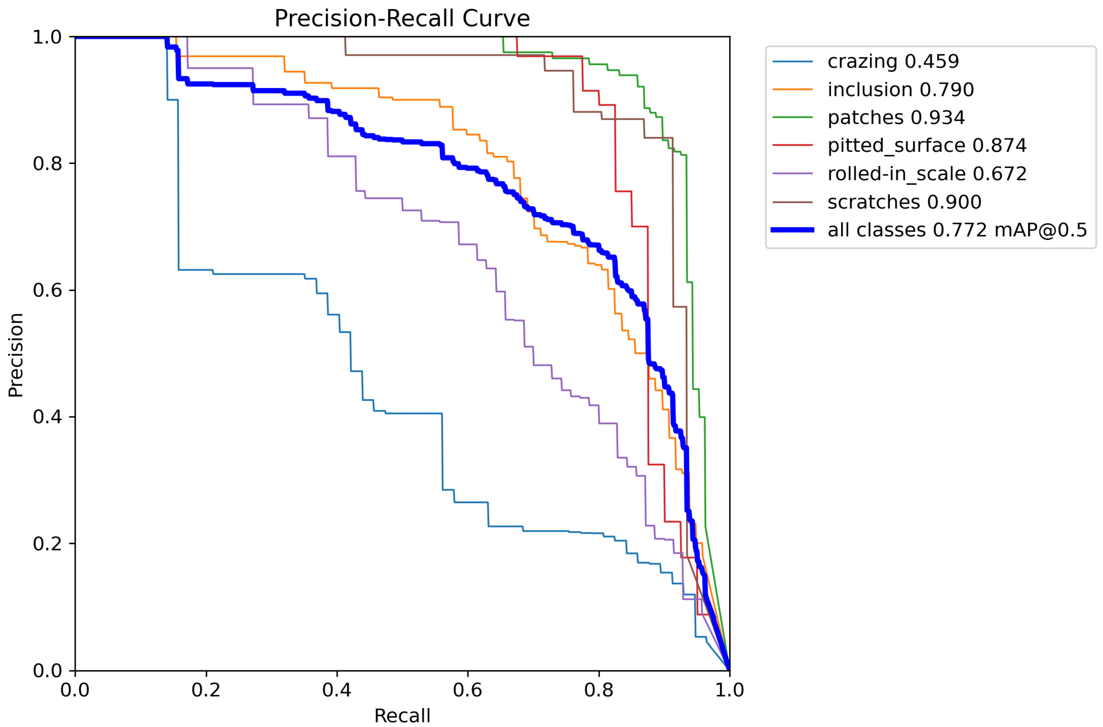
3.5. Precision–Recall Curves and Visual Predictions

Figure 11 and Figure 12 present the precision–recall (P–R) curves for the baseline YOLOv11n and the proposed YOLO-LSDI model on the test set under the same conditions. These figures show the per-class defect-detection performance as well as the overall mAP values and trends. A P–R curve closer to the top-right corner indicates a better balance between precision and recall, reflecting more accurate predictions. YOLO-LSDI clearly outperformed the baseline, with an overall mAP improvement of 5.8%. Notably, for challenging defect types like crazing and scratches, the mAP increased from 45.9% and 67.2% to 54.8% and 77.6%, respectively—an improvement of nearly 10%. Other defect categories also showed varying degrees of performance gains, demonstrating the effectiveness of the proposed enhancements.

For a clearer comparison between YOLO-LSDI and the baseline steel surface defect-detection method, both were evaluated using the NEU-DET test set. The prediction results are shown in Figure 13, with YOLOv11n’s results at the top and those of the proposed algorithm at the bottom. From the comparison, it is clear that the YOLO-LSDI algorithm has better generalization capabilities for small, fine-grained defects that are easily influenced by the background, with minimal false positives and false negatives. Overall, the YOLO-LSDI algorithm yields higher prediction confidence and effectively addresses the challenges of detecting various steel surface defects.

3.6. Confusion Matrix and Class-Wise Performance

To complement the qualitative analysis, we visualized the normalized confusion matrices of the baseline YOLOv11n and the improved YOLO-LSDI models on the NEU-DET dataset, as shown in Figure 14.

As observed, YOLO-LSDI achieved consistently higher diagonal values across most classes in the normalized confusion matrix, indicating improved true positive rates compared to the baseline YOLOv11n. For instance, the classification accuracy of the crazing class increased from 0.54 to 0.60, reflecting enhanced sensitivity to subtle surface line patterns. The patch class maintained high accuracy, with a slight improvement from 0.92 to 0.93. Despite a minor drop in accuracy for scratches (from 0.93 to 0.91), YOLO-LSDI reduced background confusion, suggesting an overall gain in defect–non-defect separability. The most notable improvements were observed in the rolled-in-scale and pitted-surface categories, which present more complex texture patterns; their correct classification rates rose from 0.73 to 0.77 and remained stable at 0.85. Additionally, false positives associated with the background class were significantly reduced, indicating that YOLO-LSDI achieved better defect-background discrimination.

These results confirm that the proposed enhancements in YOLO-LSDI, especially the attention modules, contribute to more precise and robust classification, particularly for visually similar or texture-rich defect types.

3.7. Performance of the YOLO-LSDI Algorithm on Multiple Datasets

To comprehensively evaluate YOLO-LSDI’s performance and robustness, we tested it against the baseline model on three public industrial defect datasets: GC10-DET [44] (steel surface defects), APSPC (aluminum surface defects), and PKU-Market-PC [45] (PCB defects). GC10-DET contains 2294 real steel surface images covering 10 defect types, including perforations, water spots, inclusions, and weld lines. APSPC consists of 1885 aluminum defect images across 10 categories, including dents, scratches, and coating cracks. The PCB dataset from Peking University has 1386 images featuring six defect types, including missing holes and short circuits. These datasets are widely used for industrial defect detection and classification. All experiments followed the settings in Section 3.1.

As shown in

Table 2. Generalization performance evaluation on various datasets.

Dataset	Model	Params (M)	GFLOPs	mAP@0.5 (%)	mAP@0.5:0.95 (%)	F1 (%)	FPS
GC10-DET	YOLOv11n	2.5	6.4	62.3	35.7	58.0	141.4
	YOLO-LSDI	2.6	6.1	66.5	36.8	62.2	156.3
APSPC	YOLOv11n	2.5	6.4	52.1	27.2	50.1	182.4
	YOLO-LSDI	2.6	6.1	54.2	28.7	53.4	190.7
PCB	YOLOv11n	2.5	6.4	88.3	47.5	88.7	155.5
	YOLO-LSDI	2.6	6.1	91.4	48.8	90.2	175.1

, YOLO-LSDI exhibited strong generalization across datasets. Compared to the YOLOv11n baseline, it improved the mAP@0.5 by 4.2%, 2.1%, and 3.1% on the GC10-DET, APSPC, and PCB datasets, respectively. Similarly, the mAP@0.5:0.95 rose by 1.1%, 1.5%, and 1.3%. The F1-score gains were 4.2%, 3.3%, and 1.5%, respectively. The model also reduced GFLOPs from 6.4 to 6.1 across all datasets while achieving improved inference speed. Although the parameter count slightly increased from 2.5M to 2.6M, computational efficiency remained high.

These results suggest that YOLO-LSDI holds strong potential for application in various industrial inspection scenarios, particularly those with limited computational resources.

3.8. Comparison with Mainstream Object-Detection Algorithms

We compared our proposed YOLO-LSDI algorithm with several popular detection methods on the NEU-DET dataset (

Table 3. Comparison with mainstream object-detection algorithms on the NEU-DET dataset.

Model	Params (M)	GFLOPs	mAP@0.5 (%)	mAP@0.5:0.95 (%)	F1 (%)	FPS
Faster R-CNN	136.8	251.4	76.8	43.7	68.0	45.2
SSD300	24.2	71.5	72.9	40.2	59.7	142.1
Deformable DETR	34.2	78.0	71.6	40.1	69.7	118.7
RT-DETR-R18	19.5	99.8	72.8	38.6	71.2	145.7
YOLOv5s	7.0	16.0	74.3	42.3	70.7	136.3
YOLOv7tiny	6.0	13.2	68.1	35.9	67.3	135.2
YOLOv8n	3.0	8.9	76.3	46.1	73.6	158.3
YOLOv9s	7.2	26.5	78.6	47.5	73.7	106.5
YOLO-MS-XS	4.5	8.8	77.9	48.2	74.0	141.6
YOLOv10s	8.0	24.5	70.7	40.5	68.3	180.1
YOLOv10n	2.7	8.2	73.7	41.8	69.1	220.7
YOLOv11n	2.5	6.4	77.2	45.6	72.1	158.3
YOLO-LSDI	2.7	6.1	83.0	48.0	78.3	162.1

). Two-stage detectors like Faster R-CNN show relatively high accuracy but suffer from high computational cost and slower speed. Lightweight one-stage models such as SSD300 and early YOLO versions have faster inference but lower precision, especially on small or subtle defects.

Among the YOLO series, newer versions (YOLOv8n, YOLOv9s, and YOLOv10n) improve the trade-off between speed and accuracy. Our baseline, YOLOv11n, achieves competitive results with a lightweight design.

In these comparative experiments, YOLO-LSDI outperformed all other methods, achieving the highest mAP and F1-score while maintaining real-time speed and low computational overhead. This balance confirms its suitability for practical industrial defect inspection.

As shown in

Table 4. Comparison of class-wise average precision (AP) between mainstream algorithms.

Model	AP (%)
	Cr	In	Pa	Ps	Rs	Sc
Faster R-CNN	44.1	87.4	93.0	87.7	62.3	93.3
SSD300	37.6	82.3	91.0	82.3	62.6	83.5
Deformable DETR	27.6	80.2	88.9	75.1	60.9	78.4
RT-DETR-R18	24.8	79.3	90.7	77.6	51.8	84.0
YOLOv5s	46.8	78.8	91.6	73.4	65.9	89.2
YOLOv7tiny	39.4	75.6	88.5	81.5	43.6	79.8
YOLOv8n	52.7	83.3	94.6	78.9	69.0	79.6
YOLOv9s	44.7	88.3	91.2	90.5	62.6	88.9
YOLO-MS-XS	50.7	87.5	90.2	87.1	66.9	90.5
YOLOv10s	26.7	78.6	88.7	80.1	63.6	86.2
YOLOv10n	43.9	71.3	87.7	83.9	69.0	86.4
YOLOv11n	45.9	79.0	93.4	87.4	67.2	90.0
YOLO-LSDI	54.8	90.2	95.8	87.5	77.6	92.2

Note. Cr: crazing; In: inclusions; Pa: patches; Ps: pitted surfaces; Rs: rolled-in scales; Sc: scratches.

, the proposed YOLO-LSDI algorithm achieved the best performance for key defect categories—crazing, patches, and rolled-in scales—with AP improvements of 8.9%, 2.4%, and 10.4%, respectively, over the baseline YOLOv11n. This highlights YOLO-LSDI’s enhanced ability to handle challenges like background interference and scale variability in fine-grained metal surface defect detection, ensuring its superior robustness and accuracy in industrial inspection.

In summary, YOLO-LSDI offers competitive accuracy, robustness, and generalization compared to mainstream methods, demonstrating strong potential for practical steel surface defect-detection applications.

4. Discussion

4.1. Findings and Implications

Section 2.1 describes the NEU-DET dataset, which encompasses 1800 images with a defect count of 4028. A large proportion of these defects are small targets, which pose significant challenges for detection. Therefore, the motivation for improving the model goes beyond addressing inherent limitations; it also considers the features of the dataset itself, aiming to minimize data impact. Challenges such as large-scale variations, defects influenced by the background, and similarities between different defect categories are key issues to address.

To address the challenges of steel surface defect detection, we developed targeted optimization strategies based on the characteristics of the dataset, aimed at enhancing the effectiveness of existing algorithms. We proposed four complementary improvements, each addressing specific limitations without introducing conflicts. First, the AMSPPF module, which integrates global average pooling and global max pooling to capture global context and handle scale variation, significantly improved accuracy with minimal computational overhead. Second, the DSAM attention module, combined with C2PSA, enhanced the network’s ability to focus on defect-relevant regions, particularly for fine-grained and small-scale features. Third, the standard convolution was replaced with LDConv to adaptively model irregular defect shapes while improving efficiency, reducing GFLOPs to 6.1 without sacrificing performance. Lastly, we substituted the CIoU loss function with the Inner-CIoU loss function, accelerating convergence and improving localization, especially for small or overlapping defects. Together, these strategies yielded substantial performance gains in both detection accuracy and robustness.

A comparison of the prediction results revealed that YOLO-LSDI delivered more accurate and reliable defect localization than the baseline YOLOv11, particularly in challenging scenarios involving low-contrast or irregular defect shapes. This was especially evident for defects like crazing and rolled-in scales, which are highly affected by background noise. Almost all surface defects in these categories were accurately predicted. This highlights the effectiveness of designing a unique structure to address specific cases. Of course, it is essential to maintain the model’s lightweight nature and generalization ability as much as possible.

Lastly, we did not limit ourselves to the existing approaches. We conducted comprehensive comparisons with mainstream object-detection models and their improved versions. While our model showed slight shortcomings in certain metrics, it demonstrated strong overall performance. The model achieved a favorable balance between accuracy and efficiency, maintaining its lightweight nature and demonstrating robust generalization ability across various defect scenarios. Therefore, there is still room for improvement in our model.

4.2. Limitations and Future Research Directions

This study introduced an automated approach for identifying surface defects in steel using deep learning techniques, with experimental results confirming the algorithm’s efficacy. That said, given the time limitations and the relatively nascent expertise in industrial defect detection, the current algorithm still has areas that could be refined and enhanced for real-world implementation. Consequently, this section outlines the prevailing challenges and offers a forward-looking perspective on potential avenues for future research:

• Impact of Image Quantity and Quality on Detection Performance: Surface defect detection in deep learning frameworks hinges heavily on the number and clarity of images for enhanced performance. Regarding the issue of small-sample datasets, widely used traditional data augmentation methods, such as single-image and multi-image augmentation, are often limited to simple transformations of the original data, which may not effectively enhance the diversity in the feature space of the dataset. Future work could leverage the exceptional image-generation capabilities of models like Generative Adversarial Networks (GANs) to generate highly realistic and diverse steel surface defect images. Moreover, improving image quality should start at the source, with a focus on obtaining high-quality images. Methods like image denoising could be considered to reduce information loss and improve image quality.
• Improvement of the YOLO-LSDI Algorithm: Although the proposed YOLO-LSDI algorithm resulted in some performance improvements, and strategies have been suggested to enhance its lightweight nature and generalization ability, most steel defect-detection tasks are performed in industrial environments with limited resources. These environments impose high demands on model performance, and the current work may not meet the specific requirements of certain scenarios. Therefore, future research may enhance the model using methods like pruning and knowledge distillation to better address industrial defect-detection requirements.
• Considerations for Industrial Deployment and Domain Adaptation: In real-world applications, steel surface defect-detection models are often required to operate on edge devices (e.g., NVIDIA Jetson Nano) with limited computational and memory resources. To meet these constraints, future work will consider conducting edge-deployment experiments and adopting model acceleration techniques such as quantization and TensorRT optimization. Additionally, due to the variability in steel production processes and imaging conditions across different plant sites, the generalization ability of the model becomes critical. Domain adaptation strategies—such as feature distribution alignment, adversarial training, or self-supervised domain-invariant learning—will be explored to enable the model to adapt effectively to unseen domains without extensive retraining. These efforts aim to close the gap between lab-level performance and industrial-level robustness.

5. Conclusions

This paper’s YOLO-LSDI algorithm exhibits superior performance and robust generalizability in steel surface defect-detection tasks. By addressing the inherent limitations of the model and the challenges associated with specific tasks, we introduced the AMSPPF, C2PSA-DSAM, and LDConv modules, as well as a new loss function, the Inner-CIoU, improving feature extraction efficiency, particularly in detecting small and fine-grained defects. At the same time, the model not only maintains high accuracy but also exhibits high computational efficiency and strong generalization ability. Ablation experiments validate the effectiveness of the proposed strategies, with the mAP@0.5 increasing by 5.8%, the mAP@0.5:0.95 improving by 2.4%, the F1-score rising by 6.2%, GFLOPs reduced to 6.1, and inference speed reaching 162.1 FPS. Visual results further highlight the improved detection accuracy, confidence, and reduced false detection rates across various defect types. Additionally, the model’s performance was validated on three public industrial defect-detection datasets, including GC10-DET, APSPC, and PCB datasets, where the improved model showed excellent generalization ability, with mAP@0.5 increases of 4.2%, 2.1%, and 3.1% compared to the baseline, GFLOPs reduced to 6.1, and FPS also performed well. YOLO-LSDI achieves an effective balance between computational resources, model accuracy, inference speed, and power consumption.

To conclude, the proposed YOLO-LSDI algorithm offers a practical and effective solution for steel surface defect detection by achieving a favorable trade-off between accuracy, speed, and computational efficiency. Its design makes it well-suited for real-time deployment in resource-constrained industrial environments. Although this work primarily focuses on steel defects, the underlying methodologies demonstrate potential for broader application in other small-object-detection scenarios.

While the proposed algorithm has demonstrated improvements in detection performance, several key challenges remain before it can be fully adapted for industrial applications. First, to address the limitations of small and imbalanced datasets, future work will explore the use of Generative Adversarial Networks (GANs) or similar models to generate diverse and high-fidelity steel surface defect images, thereby enhancing feature diversity and model robustness. Second, considering the computational constraints commonly present in industrial settings, lightweight optimization techniques such as model pruning and knowledge distillation will be employed to reduce model size and latency without compromising accuracy. Finally, to ensure real-world applicability across different production environments, we plan to investigate edge deployment feasibility (e.g., on devices like the Jetson Nano) and develop domain adaptation strategies. These efforts aim to improve the model’s adaptability to varying steel characteristics and imaging conditions, promoting reliable deployment in practical scenarios.

References

1. Wang, X.; Wang, Z.; Guo, C.; Han, Y.; Zhao, J.; Lu, N.; Tang, H. Application and Prospect of New Steel Corrugated Plate Technology in Infrastructure Fields. IOP Conf. Ser. Mater. Sci. Eng. 2020, 741, 012099. [Google Scholar] [CrossRef]
2. Yao, X.; Zhou, J.; Zhang, J.; Boer, C.R. From Intelligent Manufacturing to Smart Manufacturing for Industry 4.0 Driven by Next Generation Artificial Intelligence and Further On. In Proceedings of the 2017 5th International Conference on Enterprise Systems (ES), Beijing, China, 22–24 September 2017. [Google Scholar]
3. Neogi, N.; Mohanta, D.K.; Dutta, P.K. Review of vision-based steel surface inspection systems. EURASIP J. Image Video Process. 2014, 2014, 50. [Google Scholar] [CrossRef]
4. Vasan, V.; Sridharan, N.V.; Vaithiyanathan, S.; Aghaei, M. Detection and classification of surface defects on hot-rolled steel using vision transformers. Heliyon 2024, 10, e38498. [Google Scholar] [CrossRef] [PubMed]
5. Zhao, B.; Chen, Y.; Jia, X.; Ma, T. Steel surface defect detection algorithm in complex background scenarios. Measurement 2024, 237, 115189. [Google Scholar] [CrossRef]
6. Gao, X. Research on automated defect detection system based on computer vision. Appl. Comput. Eng. 2024, 101, 192–197. [Google Scholar] [CrossRef]
7. Beyerer, J.; León, F.P.; Frese, C. Machine Vision: Automated Visual Inspection: Theory, Practice and Applications; Springer: Berlin/Heidelberg, Germany, 2015. [Google Scholar]
8. Kumar, G.; Bhatia, P.K. A detailed review of feature extraction in image processing systems. In Proceedings of the 2014 Fourth International Conference on Advanced Computing & Communication Technologies, Rohtak, India, 8–9 February 2014; pp. 5–12. [Google Scholar]
9. Song, W.; Chen, T.; Gu, Z.; Gai, W.; Huang, W.; Wang, B. Wood materials defects detection using image block percentile color histogram and eigenvector texture feature. In Proceedings of the First International Conference on Information Sciences, Machinery, Materials and Energy, Chongqing, China, 11–13 April 2015; Atlantis Press: Dordrecht, The Netherlands, 2015; pp. 779–783. [Google Scholar]
10. Ma, N.; Gao, X.; Wang, C.; Zhang, Y.; You, D.; Zhang, N. Influence of hysteresis effect on contrast of welding defects profile in magneto-optical image. IEEE Sens. J. 2020, 20, 15034–15042. [Google Scholar] [CrossRef]
11. Wang, F.l.; Zuo, B. Detection of surface cutting defect on magnet using Fourier image reconstruction. J. Cent. South Univ. 2016, 23, 1123–1131. [Google Scholar] [CrossRef]
12. Li, J.H.; Quan, X.X.; Wang, Y.L. Research on defect detection algorithm of ceramic tile surface with multi-feature fusion. Comput. Eng. Appl 2020, 56, 191–198. [Google Scholar]
13. Chang, C.F.; Wu, J.L.; Chen, K.J.; Hsu, M.C. A hybrid defect detection method for compact camera lens. Adv. Mech. Eng. 2017, 9, 1687814017722949. [Google Scholar] [CrossRef]
14. Liu, Y.; Xu, K.; Xu, J. An improved MB-LBP defect recognition approach for the surface of steel plates. Appl. Sci. 2019, 9, 4222. [Google Scholar] [CrossRef]
15. Putri, A.P.; Rachmat, H.; Atmaja, D.S.E. Design of automation system for ceramic surface quality control using fuzzy logic method at Balai Besar Keramik (BBK). In Proceedings of the MATEC Web of Conferences, Malacca, Malaysia, 25–27 February 2017; EDP Sciences: Les Ulis, France, 2017; Volume 135, p. 00053. [Google Scholar]
16. Gao, X.; Xie, Y.; Chen, Z.; You, D. Fractal feature detection of high-strength steel weld defects by magneto optical imaging. Trans. China Weld. Inst. 2017, 38, 1–4. [Google Scholar]
17. Jimenez-del Toro, O.; Otálora, S.; Andersson, M.; Eurén, K.; Hedlund, M.; Rousson, M.; Müller, H.; Atzori, M. Analysis of histopathology images: From traditional machine learning to deep learning. In Biomedical Texture Analysis; Elsevier: Amsterdam, The Netherlands, 2017; pp. 281–314. [Google Scholar]
18. Zhao, X.; Wang, L.; Zhang, Y.; Han, X.; Deveci, M.; Parmar, M. A review of convolutional neural networks in computer vision. Artif. Intell. Rev. 2024, 57, 99. [Google Scholar] [CrossRef]
19. He, Y.; Song, K.; Meng, Q.; Yan, Y. An end-to-end steel surface defect detection approach via fusing multiple hierarchical features. IEEE Trans. Instrum. Meas. 2019, 69, 1493–1504. [Google Scholar] [CrossRef]
20. Damacharla, P.; Rao, A.; Ringenberg, J.; Javaid, A.Y. TLU-net: A deep learning approach for automatic steel surface defect detection. In Proceedings of the 2021 International Conference on Applied Artificial Intelligence (ICAPAI), Halden, Norway, 19–21 May 2021; pp. 1–6. [Google Scholar]
21. Bhatt, P.M.; Malhan, R.K.; Rajendran, P.; Shah, B.C.; Thakar, S.; Yoon, Y.J.; Gupta, S.K. Image-based surface defect detection using deep learning: A review. J. Comput. Inf. Sci. Eng. 2021, 21, 040801. [Google Scholar] [CrossRef]
22. Zhao, W.; Chen, F.; Huang, H.; Li, D.; Cheng, W. A new steel defect detection algorithm based on deep learning. Comput. Intell. Neurosci. 2021, 2021, 5592878. [Google Scholar] [CrossRef]
23. Liu, Q.; Wang, C.; Li, Y.; Gao, M.; Li, J. A fabric defect detection method based on deep learning. IEEE Access 2022, 10, 4284–4296. [Google Scholar] [CrossRef]
24. Zhao, C.; Shu, X.; Yan, X.; Zuo, X.; Zhu, F. RDD-YOLO: A modified YOLO for detection of steel surface defects. Measurement 2023, 214, 112776. [Google Scholar] [CrossRef]
25. Yi, F.; Zhang, H.; Yang, J.; He, L.; Mohamed, A.S.A.; Gao, S. YOLOv7-SiamFF: Industrial defect detection algorithm based on improved YOLOv7. Comput. Electr. Eng. 2024, 114, 109090. [Google Scholar] [CrossRef]
26. Xie, W.; Sun, X.; Ma, W. A light weight multi-scale feature fusion steel surface defect detection model based on YOLOv8. Meas. Sci. Technol. 2024, 35, 055017. [Google Scholar] [CrossRef]
27. Zou, J.; Wang, H. Steel Surface Defect Detection Method Based on Improved YOLOv9 Network. IEEE Access 2024, 12, 124160–124170. [Google Scholar] [CrossRef]
28. Ruengrote, S.; Kasetravetin, K.; Srisom, P.; Sukchok, T.; Kaewdook, D. Design of Deep Learning Techniques for PCBs Defect Detecting System based on YOLOv10. Eng. Technol. Appl. Sci. Res. 2024, 14, 18741–18749. [Google Scholar] [CrossRef]
29. Tang, H.; Li, Z.; Zhang, D.; He, S.; Tang, J. Divide-and-Conquer: Confluent Triple-Flow Network for RGB-T Salient Object Detection. IEEE Trans. Pattern Anal. Mach. Intell. 2025, 47, 1958–1974. [Google Scholar] [CrossRef] [PubMed]
30. Bao, Y.; Song, K.; Liu, J.; Wang, Y.; Yan, Y.; Yu, H.; Li, X. Triplet-Graph Reasoning Network for Few-Shot Metal Generic Surface Defect Segmentation. IEEE Trans. Instrum. Meas. 2021, 70, 5011111. [Google Scholar] [CrossRef]
31. Khanam, R.; Hussain, M. Yolov11: An overview of the key architectural enhancements. arXiv 2024, arXiv:2410.17725. [Google Scholar]
32. Jocher, G.; Chaurasia, A.; Qiu, J. Ultralytics YOLO, Version 8.0.0. 2023. Available online: https://github.com/ultralytics/ultralytics (accessed on 14 June 2025).
33. Wang, A.; Chen, H.; Liu, L.; Chen, K.; Lin, Z.; Han, J.; Ding, G. Yolov10: Real-time end-to-end object detection. arXiv 2024, arXiv:2405.14458. [Google Scholar]
34. Howard, A.G.; Zhu, M.; Chen, B.; Kalenichenko, D.; Wang, W.; Weyand, T.; Andreetto, M.; Adam, H. MobileNets: Efficient convolutional neural networks for mobile vision applications. arXiv 2017, arXiv:1704.04861. [Google Scholar]
35. Lin, T.Y.; Maire, M.; Belongie, S.; Hays, J.; Perona, P.; Ramanan, D.; Dollár, P.; Zitnick, C.L. Microsoft coco: Common objects in context. In Proceedings of the Computer Vision–ECCV 2014: 13th European Conference, Zurich, Switzerland, 6–12 September 2014; Proceedings, Part V 13. Springer: Berlin/Heidelberg, Germany, 2014; pp. 740–755. [Google Scholar]
36. He, K.; Zhang, X.; Ren, S.; Sun, J. Spatial pyramid pooling in deep convolutional networks for visual recognition. IEEE Trans. Pattern Anal. Mach. Intell. 2015, 37, 1904–1916. [Google Scholar] [CrossRef]
37. Jocher, G.; Chaurasia, A.; Stoken, A.; Borovec, J.; Kwon, Y.; Michael, K.; Fang, J.; Yifu, Z.; Wong, C.H.; Montes, D.; et al. YOLOv5 by Ultralytics, Version 7.0. 2020. Available online: https://github.com/ultralytics/yolov5 (accessed on 14 June 2025).
38. Woo, S.; Park, J.; Lee, J.Y.; Kweon, I.S. Cbam: Convolutional block attention module. In Proceedings of the European Conference on computer vision (ECCV), Munich, Germany, 8–14 September 2018; pp. 3–19. [Google Scholar]
39. Zhu, L.; Wang, X.; Ke, Z.; Zhang, W.; Lau, R.W. Biformer: Vision transformer with bi-level routing attention. In Proceedings of the IEEE/CVF Conference on Computer Vision and Pattern Recognition, Vancouver, BC, Canada, 17–24 June 2023; pp. 10323–10333. [Google Scholar]
40. Zhang, X.; Song, Y.; Song, T.; Yang, D.; Ye, Y.; Zhou, J.; Zhang, L. LDConv: Linear deformable convolution for improving convolutional neural networks. Image Vis. Comput. 2024, 149, 105190. [Google Scholar] [CrossRef]
41. Yu, J.; Jiang, Y.; Wang, Z.; Cao, Z.; Huang, T. Unitbox: An advanced object detection network. In Proceedings of the 24th ACM international conference on Multimedia, Amsterdam, The Netherlands, 15–19 October 2016; pp. 516–520. [Google Scholar]
42. Zheng, Z.; Wang, P.; Ren, D.; Liu, W.; Ye, R.; Hu, Q.; Zuo, W. Enhancing geometric factors in model learning and inference for object detection and instance segmentation. IEEE Trans. Cybern. 2021, 52, 8574–8586. [Google Scholar] [CrossRef]
43. Zhang, H.; Xu, C.; Zhang, S. Inner-IoU: More effective intersection over union loss with auxiliary bounding box. arXiv 2023, arXiv:2311.02877. [Google Scholar]
44. Lv, X.; Duan, F.; Jiang, J.j.; Fu, X.; Gan, L. Deep Metallic Surface Defect Detection: The New Benchmark and Detection Network. Sensors 2020, 20, 1562. [Google Scholar] [CrossRef] [PubMed]
45. Huang, W.; Wei, P. A PCB Dataset for Defects Detection and Classification. arXiv 2019, arXiv:1901.08204. [Google Scholar]
Figure 1. Typical images of six defect types.
Electronics 14 02576 g001
Figure 2. Specific distribution of defect quantities and the area ratio of the defect region in each image of the dataset.
Electronics 14 02576 g002
Figure 3. Network architecture of the YOLOv11 algorithm. The model incorporates the C3K2 module in the backbone for enhanced feature representation, utilizes the SPPF module for efficient multi-scale feature aggregation, and employs the C2PSA module in the neck to improve channel-wise attention.
Electronics 14 02576 g003
Figure 4. Network architecture of the improved YOLO-LSDI model. Compared to the original YOLOv11, the SPPF module is replaced with the AMSSPPF module for enhanced multi-scale context extraction, standard convolution is replaced with LDConv to reduce computational cost, and the C2PSA attention module is upgraded to the C2PSA-DSAM for improved feature refinement.
Electronics 14 02576 g004
Figure 5. The structures of the SPP, SPPF, and improved AMSPPF modules. (a) Structure of the original SPP module, showing how different pooling kernels are applied to the feature maps and concatenated for fusion. (b) Structure of the SPPF module, where 5 × 5 max-pooling layers are used to extract features at multiple scales and improve accuracy. (c) Structure of the AMSPPF module, demonstrating the inclusion of global average-pooling and global max-pooling layers to incorporate both edge and background information, along with the final concatenation step.
Electronics 14 02576 g005
Figure 6. Replacing the CAM with Deformable Bi-level Routing Attention (DBRA) and combining it with the SAM to form the new attention mechanism, the DSAM.
Electronics 14 02576 g006
Figure 7. The architecture of the C2PSA-DSAM, consisting of multiple stacked PSABlockDSAM units. The input feature X i n is first processed by a 1 × 1 convolution and split into multiple branches, each passing through a PSABlockDSAM. These outputs are concatenated and refined through another 1 × 1 convolution. The PSABlockDSAM enhances features via the DSAM attention mechanism, followed by two sequential 1 × 1 convolutions and a residual connection to yield the output X o u t . This design enables adaptive feature recalibration and improves defect localization sensitivity.
Electronics 14 02576 g007
Figure 8. Schematic illustration of the structure of LDConv. The module initializes a set of sampling coordinates for a convolution with an arbitrary kernel size and dynamically adjusts the sampling pattern using learnable offsets. As a result, the sampling locations are adaptively resampled at each spatial position, enabling flexible and content-aware receptive fields.
Electronics 14 02576 g008
Figure 9. Schematic representation of the Inner-CIoU loss function in object detection. (Left) The target box (solid blue line) and its inner target box (solid orange line) are aligned with the ground-truth box (red dot). The inner target box is defined by reducing the width ( w i n n e r ) and height ( h i n n e r ) of the original target box. (Right) The anchor box (dashed blue line) and its inner anchor box (dashed orange line) are similarly aligned with the ground-truth box. The center coordinates ( x c , y c ) and the ground-truth box coordinates ( x c g t , y c g t ) are marked. This visualization demonstrates how the Inner-CIoU loss function enhances the precision of object detection by focusing on the inner regions of bounding boxes.
Electronics 14 02576 g009
Figure 10. Visualization of attention heatmaps for selected steel surface defect types, comparing the baseline YOLOv11 model and models enhanced with the proposed modules. (ac) Heatmaps generated by the baseline model for (a) patches, (b) crazing, and (c) inclusion defects. (df) Corresponding heatmaps after adding (d) AMSPPF for patches, (e) DSAM for crazing, and (f) LDConv for inclusions. The enhanced modules demonstrate improved focus on defect regions, clearer boundaries, and better discrimination of fine-grained features.
Electronics 14 02576 g010
Figure 11. P–R curve of the YOLOv11n algorithm.
Electronics 14 02576 g011
Figure 12. P–R curve of the YOLO-LSDI algorithm.
Electronics 14 02576 g012
Figure 13. Prediction results on the NEU-DET dataset.The red arrows highlight defect regions that the improved model successfully detects whereas the baseline model fails to identify.
Electronics 14 02576 g013
Figure 14. Normalized confusion matrices of the baseline YOLOv11n (left) and the proposed YOLO-LSDI (right) on the NEU-DET dataset. The darker diagonal values for YOLO-LSDI indicate improved class-wise accuracy.
Electronics 14 02576 g014