ISELDP: An Enhanced Dropout Prediction Model Using a Stacked Ensemble Approach for In-Session Learning Platforms

Abstract

High dropout rates remain a significant challenge in Massive Open Online Courses (MOOCs), making early identification of at-risk students crucial. This study introduces a novel approach called In-Session Stacked Ensemble Learning for Dropout Prediction (ISELDP), which predicts student dropout during course sessions by combining multiple base learners—Adaptive Boosting (AdaBoost), Random Forest (RF), Extreme Gradient Boosting (XGBoost), and Gradient Boosting—into a stacked ensemble with a Multi-Layer Perceptron (MLP) serving as the meta-learner. To optimise model performance, hyperparameters were tuned using Grid Search. The proposed method was evaluated under two scenarios using in-session student interaction data, one with imbalanced data and another with balanced data. Results demonstrate that ISELDP achieves an average accuracy of 88%, outperforming individual baseline models with improvements of up to 2% in accuracy and 2.4% in F1-score.

1. Introduction

Massive Open Online Courses (MOOCs) have transformed education by offering scalable access to learning resources and opportunities for skill development. However, persistently high dropout rates—where many students leave courses before completion—remain a significant challenge for MOOC platforms [1]. To address this issue, dropout prediction has emerged as a critical area of study, aiming to identify students at risk of disengaging.

Dropout is a complex phenomenon that is affected by a number of institutional, environmental, and personal factors. According to certain psychological theories, acknowledged competence, independence, and connection are necessary for continuous engagement [1]. Predictive modelling frequently uses behavioural indicators such as assignment completion and engagement frequency as substitutes for these features in educational environments [2]. By combining features that reflect learner engagement, performance patterns, and temporal behaviour, this study aims to develop a method that will allow for early detection of disengagement indicators that could result in dropout.

Machine learning (ML) approaches, particularly ensemble methods, have shown promise in predicting student dropout. However, a major limitation is the inherent class imbalance in MOOC datasets, where non-dropouts significantly outnumber dropouts [2]. This imbalance can result in biased models that favour the majority class, reducing the accuracy of predictions for the minority class—those most at risk of dropping out. Additionally, the presence of irrelevant or redundant features in the dataset can further degrade model performance.

The challenge is especially pronounced in in-session learning models, where predicting dropout becomes more difficult due to the predominance of non-dropout data [2]. Traditional dropout prediction models often fail to adequately address this imbalance, resulting in suboptimal performance when identifying at-risk students [3]. Furthermore, the inclusion of unnecessary variables can hinder the development of reliable early prediction systems, ultimately lowering predictive accuracy [4].

Another critical issue in existing dropout prediction models is overfitting. Many models perform well on training data but fail to generalise effectively to unseen data, particularly when noisy or irrelevant features are present [5]. Although classification algorithms are widely used in dropout prediction, these models may be prone to overfitting if proper feature selection and hyperparameter tuning are not conducted [6]. To overcome these limitations, this study proposes a stacked ensemble learning framework that integrates several base classifiers with a Multi-Layer Perceptron (MLP) as the meta-learner, aiming to improve predictive accuracy and robustness in dropout prediction.

1.1. Motivations

High dropout rates remain a significant challenge for in-session learning, undermining its effectiveness and long-term sustainability. Existing methods often struggle with issues such as data imbalance and the complexities of real-time (in-session) prediction. Therefore, improved predictive frameworks are essential to enhance course completion rates and provide better learner support. The key motivations for conducting this study are outlined below:

▪

Enhancing in-session prediction: Traditional single classifiers often lack the ability to generalise effectively. This study leverages stacked ensemble learning to combine the strengths of multiple models for more robust in-session dropout prediction.

▪

Addressing data imbalance: The study explores advanced ensemble strategies designed to mitigate the performance degradation caused by class imbalance, a common issue on in-session datasets.

▪

Optimising the meta-learner: Through careful hyperparameter tuning, the stacked architecture is refined to maximise performance, ensuring that the meta-learner contributes meaningfully to overall prediction accuracy.

1.2. Contributions

Compared to conventional methodologies, this study presents a comprehensive solution that enhances prediction accuracy on in-session datasets by developing a novel, fine-tuned stacked ensemble learning framework for dropout prediction. The main contributions of this research are as follows:

▪

Development of a stacked ensemble architecture: An efficient predictive model is constructed by integrating four robust base learners—Adaptive Boosting (AdaBoost), Random Forest (RF), Extreme Gradient Boosting (XGBoost), and Gradient Boosting Classifier (GBC)—to optimise prediction outcomes.

▪

Integration of MLP as a meta-learner: A Multi-Layer Perceptron (MLP) is used as the meta-learner to capture complex nonlinear relationships between the base model outputs, significantly improving classification accuracy.

▪

Hyperparameter tuning using Grid Search: Grid Search is employed to systematically tune the parameters of both the base learners and the meta-learner, resulting in significant improvements in precision, recall, and F1-score across different scenarios.

In addition, the study evaluates the proposed model’s performance under both imbalanced and balanced data conditions to simulate realistic learning environments. Based on these contributions, the research explores the potential of advanced ensemble learning techniques to improve dropout prediction accuracy for in-session datasets. The study is guided by the following research questions (RQs).

▪

RQ1: How effective is a stacked ensemble learning model, combining multiple base classifiers with an MLP meta-learner, in predicting student dropout during in-session platform activity?

▪

RQ2: To what extent does hyperparameter tuning via Grid Search enhance the performance of the stacked ensemble model under different data scenarios, including imbalanced and balanced datasets?

▪

RQ3: Can feature selection improve both the predictive capability and interpretability of the dropout prediction model when applied to balanced datasets?

▪

RQ4: What impact do resampling strategies and cost-sensitive learning approaches have on mitigating class imbalance in in-session dropout prediction?

In addressing these questions, the study aims to advance dropout prediction strategies for in-session learning platforms by leveraging the advantages of stacked ensemble learning methods.

The remainder of this paper is organised as follows: Section 2 presents a review of related work, focusing on recent contributions in stacked ensemble learning approaches; Section 3 introduces the proposed framework and outlines the mathematical foundations of the base and meta models; Section 4 details the study methodology; Section 5 discusses the simulation setup and evaluates the performance of the proposed approach; and Section 6 concludes the study and outlines directions for future research.

2. Related Work

In recent years, dropout prediction in online learning platforms has gained significant attention. Various machine learning (ML) approaches have been employed for early dropout prediction, including decision trees (DTs), Support Vector Machines (SVMs), and Deep Learning (DL) models [7]. Ensemble learning techniques, such as Random Forest (RF) and Gradient Boosting Classifier (GBC), have demonstrated improved predictive performance by combining the strengths of multiple classifiers. However, challenges such as class imbalance, inadequate feature engineering, and insufficient integration among base learners still limit the effectiveness of current methods [8].

More recently, some studies have explored the use of stacked ensemble frameworks that integrate systematic hyperparameter optimisation with a meta-learner, such as a Multi-Layer Perceptron (MLP) [9].

Table 1. Comprehensive comparison for the related studies with our proposed approach.

Citations	Contribution	Methodology	Dataset	Highlights
[10]	Multi-Model Stacking Ensemble to improve MOOC dropout prediction.	Two-layer stacking using an XGBoost meta-classifier for feature prediction from student logs.	KDDcup2015	Accuracy up to 88%
[11]	Adapted dropout prediction models for in-session school platforms.	MLP-based model using step-wise session data and personalised intervention design	In-session dataset	Accuracy with 87%
[12]	Developed an ensemble model using real-time data to reduce dropout and personalise learning.	Ensemble of LGBM, XGB, and RF with MLP meta-classifier	Blackboard dataset	High student success rate
[13]	Predicted dropout using multiple algorithms on university data	Compares LR, RF, and LightGBM by using oversampling with SMOTE, ADASYN	Sahmyook University platform	Weak ensemble model stacking
[14]	Developed a stacking ensemble for early MOOC dropout prediction	Combines classifiers into a stacked model	NA	Weak meta-learner optimisation
[15]	Developed a stacking-based ML model to predict student performance on e-learning platforms	Combines nearest neighbour (NN), DT, RF XGBoost, Naive Bayes (NB), and LR	OULAD and Deeds datasets	Boost accuracy by 4% compared to the conventional methods

summarises these studies, outlining their key contributions and limitations.

For example, in [10], the authors proposed a Multi-Model Stacking Ensemble for improving dropout prediction accuracy on MOOC platforms. Their two-layer stacking model trained five base classifiers in the first layer, with XGBoost serving as the meta-classifier in the second layer. Evaluated on the KDDCup2015 dataset using weekly features extracted from student log data, the model outperformed single-model approaches in terms of predictive accuracy.

A study in [11] adapted traditional MOOC dropout prediction methods for in-session dropout prediction within school-supportive learning platforms. They developed time-progressive ML models, including MLPs, using over 164,000 session logs from 52,000 users on an online language platform. By identifying motivational and subject-specific patterns, their model achieved up to 87% accuracy, enabling personalised, real-time interventions based on dropout probabilities.

In [12], the authors introduced a Stacked Generalisation for Failure Prediction model aimed at reducing student failure in online learning environments. Their approach combined three ensemble classifiers, RF, XGBoost (XGB), and LightGBM (LGBM), with an MLP as the meta-classifier. The model led to a significant reduction in dropout rates and a success rate of 98.86%, highlighting the potential of ensemble learning for enhancing educational outcomes.

At Sahmyook University [13], a study proposed a dropout prediction model using several ML techniques, including DT, RF, SVM, LightGBM, and Logistic Regression (LR). The study, based on data from over 20,000 students, applied oversampling techniques such as SMOTE, ADASYN, and Borderline-SMOTE to address class imbalance. Among the models evaluated, LightGBM achieved the best performance on imbalanced data with an F1-score of 0.840, surpassing the other algorithms.

A stacking ensemble machine learning (ML) approach was proposed in [14] to address high dropout rates in MOOCs and to identify at-risk students early in the course. The proposed method, which integrated several classifiers into a stacked ensemble, outperformed traditional ML models and achieved a high prediction accuracy of 93.4%.

Similarly, a study in [15] focused on predicting student success based on behavioural data from e-learning platforms. Their approach combined weak learners, such as K-Nearest Neighbours (KNN), decision tree (DT), Random Forest (RF), XGBoost, Naive Bayes (NB), and Logistic Regression (LR), as base models, with LR selected as the meta-learner. The model achieved accuracies of 98% on the OULAD dataset and 87% on the DEEDs dataset.

Dropout is still a problem in a variety of educational contexts, even though a lot of recent research on dropout prediction has focused on MOOC environments because of the wide range of interaction data available [10,15]. Recent research has highlighted the significance of making dropout models in the context of particular educational environments, focusing on differences in institutional support, and learner motivation.

Furthermore, while ML has shown potential in detecting students who are at risk, a number of studies have highlighted its drawbacks, including its ability to overfit to existing behavioural patterns, low generalisability across institutions, and being unable to be interpreted when making important educational decisions [15]. ML-based stacked ensemble learning, on the other hand, will achieve notable improvements in such scenarios.

Findings from these related works indicate that stacked ensemble learning approaches are highly effective in predicting student dropout in both MOOC and in-session datasets. However, despite these advances, class imbalance remains a significant challenge in dropout prediction [16]. Unbalanced datasets can result in biased models that favour the majority class, leading to poor generalisation for the minority (at-risk) class.

To address this issue, the present study employs an under-sampling technique to balance class distribution in the in-session dataset [17]. It builds upon the methodology used in prior work such as that in [11], which used time-progressive ML models for in-session dropout prediction. In that study, an MLP model using sequential learning data achieved dropout prediction accuracy of up to 87%.

The methodology in [11] is used in this study as a benchmark for evaluating the performance, precision, and adaptability of the proposed approach. Additionally, comparisons with other structurally similar methods allow for a more comprehensive evaluation of the proposed model’s robustness and generalisability.

3. Proposed Models

Stacked ensemble learning is a hierarchical machine learning (ML) architecture that combines multiple base models with a meta-learner to enhance predictive performance [12]. This approach leverages the strengths of various classifiers while mitigating their individual weaknesses, resulting in more robust and accurate predictions. The core objective is for the meta-learner to learn the optimal way to integrate the outputs of the base models, thereby improving generalisation and overall accuracy.

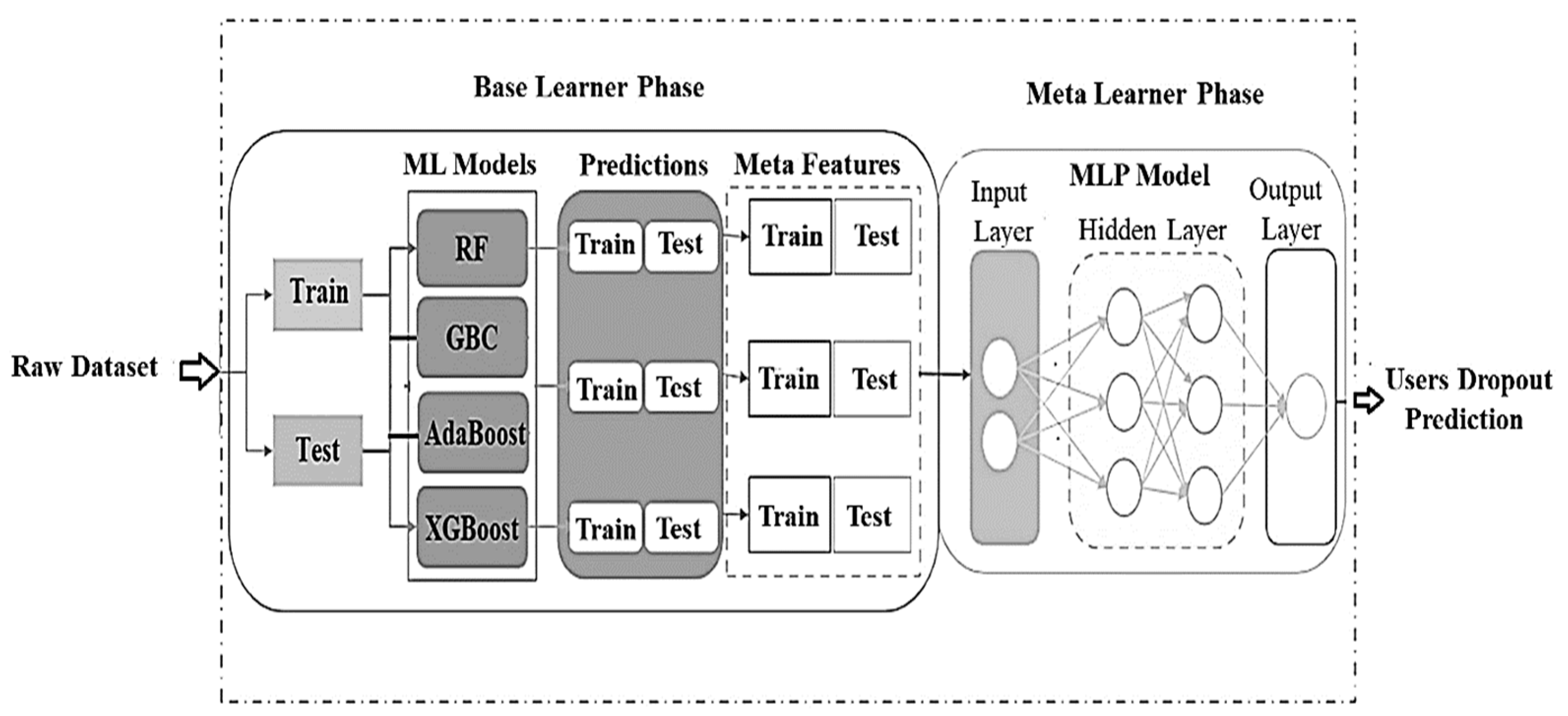
The proposed approach adopts a stacked ensemble learning architecture to improve dropout prediction performance across multiple stages, as illustrated in Figure 1. It consists of four base learner models integrated with a meta-learner to predict student dropout in an in-session dataset. This dataset, consisting of approximately 60 sentences, offers a valuable opportunity to observe student behaviour and assess dropout risk in real-time learning environments.

▪

Phase (1): Base Model Training

The original labelled dataset $D{\left\{\left(x_i,y_i\right)\right\}}_{i=1}^N$ is divided into training and testing subsets as shown in Figure 1. Using the original training dataset D, a collection of varied base classifiers, ${\left\{f_j\left(\mathrm{x}\right)\right\}}_{j=1}^k$, is learned. To ensure variety, which is essential for ensemble performance, these models might have different hyperparameters [13]. A unique mapping from input features $x_i$ to output labels $y_i$ is learned by each base classifier.

▪

Phase (2): Probability Prediction

Each base classifier $f_j$ produces class probability estimates instead of concrete labels after training. This occurs effectively for both the test and training instances. A vector of predicted probabilities $f_j\left(x_i\right)$ = [$p_{i,1}^j$, $p_{i,2}^j$, …$p_{i,c}^j$], where c is the number of classes, represents the output of each base model for a given sample $x_i$ [14]. These probabilistic approaches offer a more comprehensive depiction of predictions and capture model confidence.

▪

Phase (3): Feature Augmentation

To produce an enhanced feature set, the original input features $x_i$ have been combined with the predicted probability vectors from each base classifier [14]. The new feature vector is as follows for every sample.

$$x_i^{aug}=[x_i,\left(f_1\right(x_i), f_2\left(x_i\right), \dots \dots \dots . f_n\left(x_i\right)]$$

(1)

This process increases the input’s representational capability by incorporating both the raw data and the meta-level knowledge that the base models have gained.

▪

Phase (4): Meta-Learner Training

The last stage, represented by the meta-learner, involves using the enhanced features to train an MLP model. The enhanced dataset ${\left\{\left(x_i^{aug},y_i\right)\right\}}_{i=1}^N$ is used to train a final classifier, usually MLP represented as g(⋅) [15]. To produce the final predictions, this meta-learner makes use of the combined information from the basic models and the original features. Its objective is to figure out how to best integrate the basic models’ outputs to make the best decisions. The outputs from several base learners are fed into a meta-learner g (⋅) to provide the final prediction, $\widehat{\mathrm{y}}$, for a stacked ensemble framework. To capture its prediction confidence, each base learner $f_j\left(x\right)$ produces a probability distribution across the target classes [16]. The following is a mathematical representation of the final model prediction.

$$\widehat{y}=\mathrm{g} \left[f_1\right(x), f_2\left(x\right), \dots \dots \dots . f_n\left(x\right)]$$

(2)

where the input feature vector is denoted by x. The number of base models is denoted by n. The probability forecasts from the j-th base model are represented by $f_j\left(x\right)$. The final prediction $\widehat{y}$ is produced by the meta-learner g (⋅) for MLP, which is trained on the concatenated probability outputs and optionally the original features.

3.1. Selected Base Models

In the proposed stacked ensemble learning model, the diversity and predictive accuracy of the base learners play a critical role in the overall performance. To achieve this, a set of advanced tree-based ensemble algorithms is employed, including AdaBoost, Random Forest (RF), Extreme Gradient Boosting (XGBoost), and Gradient Boosting Classifier (GBC) [17]. These algorithms were chosen for their robust learning paradigms, scalability, and strong performance in classification accuracy and model generalisation. The selection of these four base learners is based on the following considerations:

▪

Complementary learning strategies: RF minimises variance through bagging, while boosting techniques, such as AdaBoost, XGBoost, and GBC, focus on reducing bias.

▪

Tree-based structure: All models are tree-based, enabling them to naturally capture complex, nonlinear decision boundaries.

▪

Uncorrelated error predictions: Incorporating multiple boosting models increases the likelihood of generating uncorrelated errors, which enhances the effectiveness of the meta-learner.

▪

Scalability and accuracy: These models deliver reliable results across both small and large datasets.

Collectively, these base learners bring complementary strengths to the ensemble, allowing the meta-learner to integrate their outputs and produce more accurate and generalisable predictions.

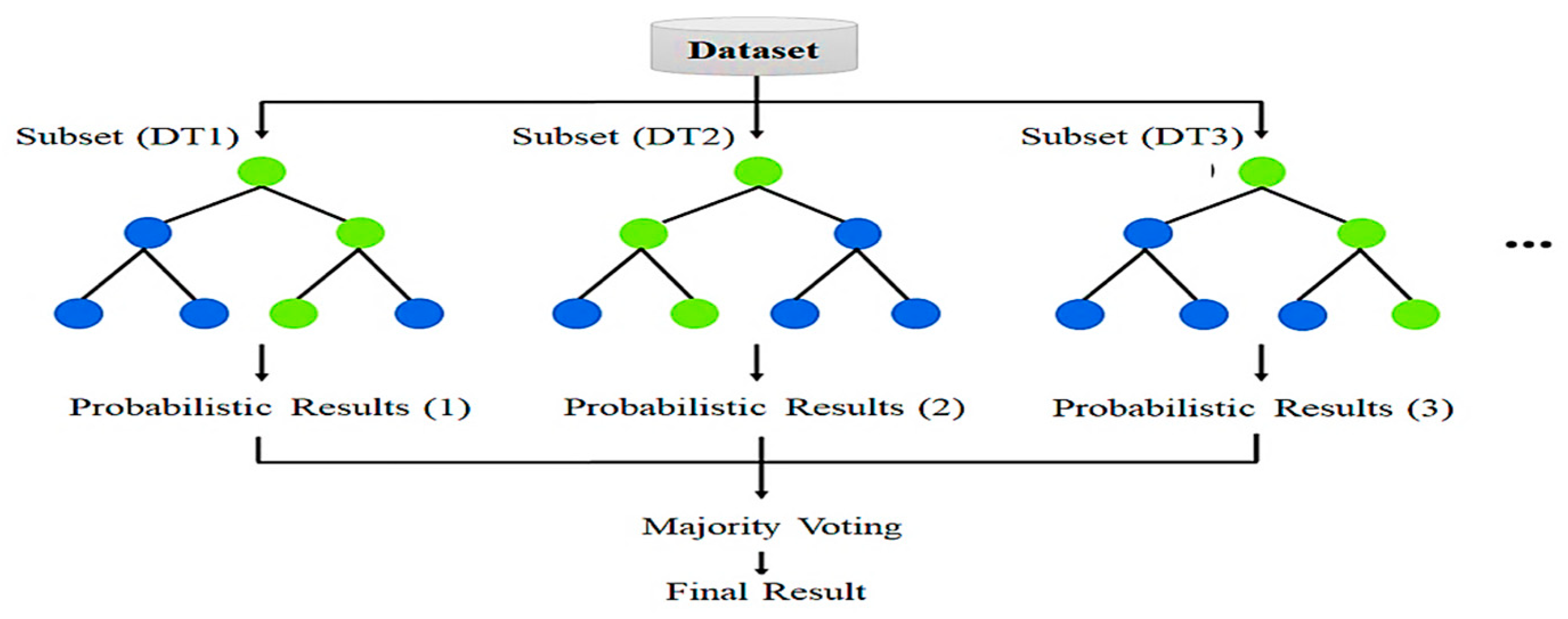
3.1.1. Random Forest

An ensemble of decision trees known as RF was trained through the use of boosting techniques. A random subset of the training data is used to train each tree, and a random subset of features is taken into consideration at each tree split as shown in Figure 2. By adding randomisation to the feature space and data, this improves generalisation and reduces overfitting [18]. If the t-th decision tree in the forest is represented by the $h_t\left(X\right)$ in RF, the final prediction $P_{RF}$(x) for classification tasks can be calculated as follows [19].

$$P_{RF} \left(\mathrm{x}\right)=\mathrm{mode} \left\{h_1\right(X), h_2\left(X\right), \dots \dots , h_T\left(X\right)\}$$

(3)

where T is the total tree count of the forest. The average of all tree predictions for regression is calculated by Equation (4). A baseline sample of the dataset is used to train each tree, and only a random subset of features is taken into account at each split. Randomness is added, which improves generalisation and reduces overfitting. Using multiple decision trees trained on baseline samples is made possible by the use of RF of the model.

$$P_{RF} (x)={\displaystyle \frac{1}{T}}{\sum }_{t=1}^T{h}_t\left(X\right)$$

(4)

For the in-session dataset, the RF works especially well because of its ability to manage noisy data and irrelevant features [19]. Significant factors contributing to dropout risk, such as difficulty, can be found using RF feature importance calculation. RF ensures consistent performance across all given dataset features by averaging predictions from various trees, even in cases where individual data subsets give imbalance or variation.

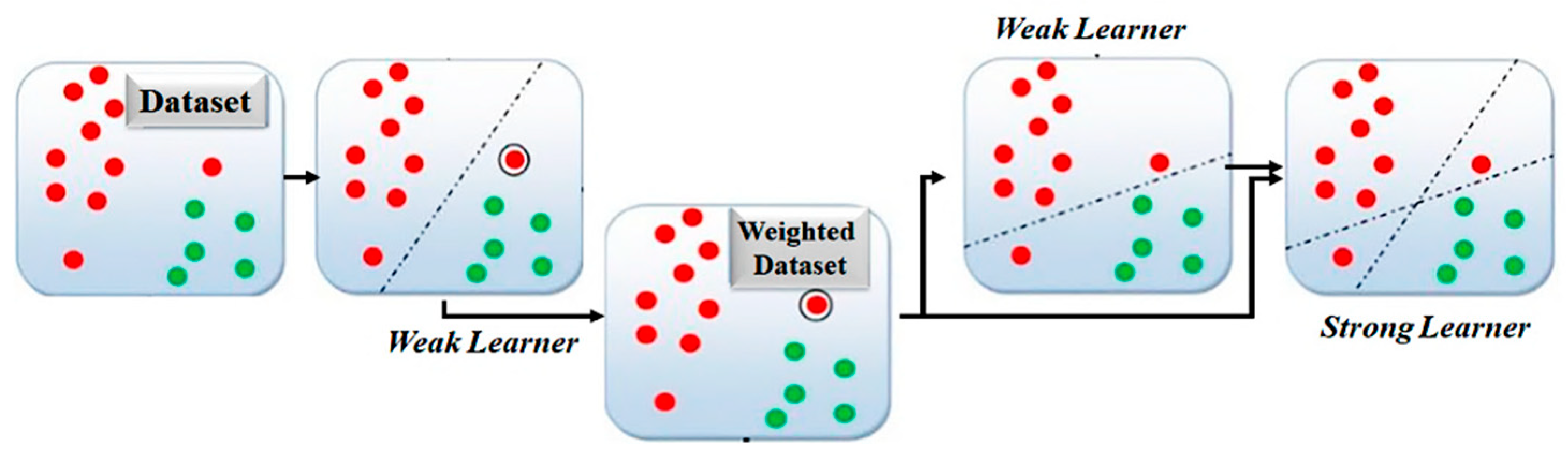
3.1.2. Adaptive Boosting Classifier

AdaBoost is a sequential ensemble technique that creates an effective classifier by combining several weak learners, usually decision stumps. By varying the weights of observations in each iteration, it focuses on the training cases that are most challenging to classify [20]. Figure 3 shows the general concept about AdaBoost process flow. Higher weights are assigned to misclassified samples, which directs later models to fix those mistakes. The weighted majority decision of the weak learners determines the final prediction. The weak classifier at iteration t in the AdaBoost model is denoted by $h_t\left(x\right)$ [14,20]. The following equation can be used to calculate the final prediction $P_{AB}$(x).

$$P_{AB} (\mathrm{x})=\mathit{sign} \left({\sum }_{t=1}^T{\alpha }_t{h}_t\left(X\right)\right)$$

(5)

In Equation (5), ${\alpha }_t$ represents each weak learner’s weight that depends on the weighted error rate ${ϵ}_t$ of the t-th weak classifier. The weak learner’s weight and error rate can be calculated by the following equations:

$${\alpha }_t={\displaystyle \frac{1}{2}}\mathit{ln} \left({\displaystyle \frac{1-{ϵ}_t}{{ϵ}_t}}\right)$$

(6)

$${ϵ}_t={\displaystyle \frac{{\sum }_{i=1}^n{w}_i^{\left(t\right)} {\delta }_{y_i\ne h_i\left(x_i\right)}}{{\sum }_{i=1}^n{w}_i^{\left(t\right)}}}$$

(7)

In Equation (7), $w_i^{\left(t\right)}$ represents the weight of the i-th instance at iteration t. ${\delta }_{y_i\ne h_i\left(x_i\right)}$ shows if the i-th instance has been incorrectly classified (1 if incorrectly classed, 0 if correctly classified) [20]. Following each iteration, the instance weights are modified as follows.

$$w_i^{(t+1)}=w_i^{\left(t\right)}\exp (-{\alpha }_t{y}_i{h}_i\left(x_i\right)).$$

(8)

where the true label of the i-th instance in the collection is denoted by $y_i$. Additionally, for iteration t, the weak classifier $h_t$ predicts the label for the i-th instance, which is represented by $h_i\left(x_i\right)$.

AdaBoost plays a crucial role in the proposed approach by highlighting how the number of pending tasks influences the probability of student dropout. It addresses challenges posed by imbalanced datasets by giving more weight to minority-class instances, specifically, students at risk of dropping out, thereby improving recall in dropout prediction [20]. Through its iterative learning process, AdaBoost is able to capture subtle patterns that other models might overlook and adapt effectively to changes in student behaviour.

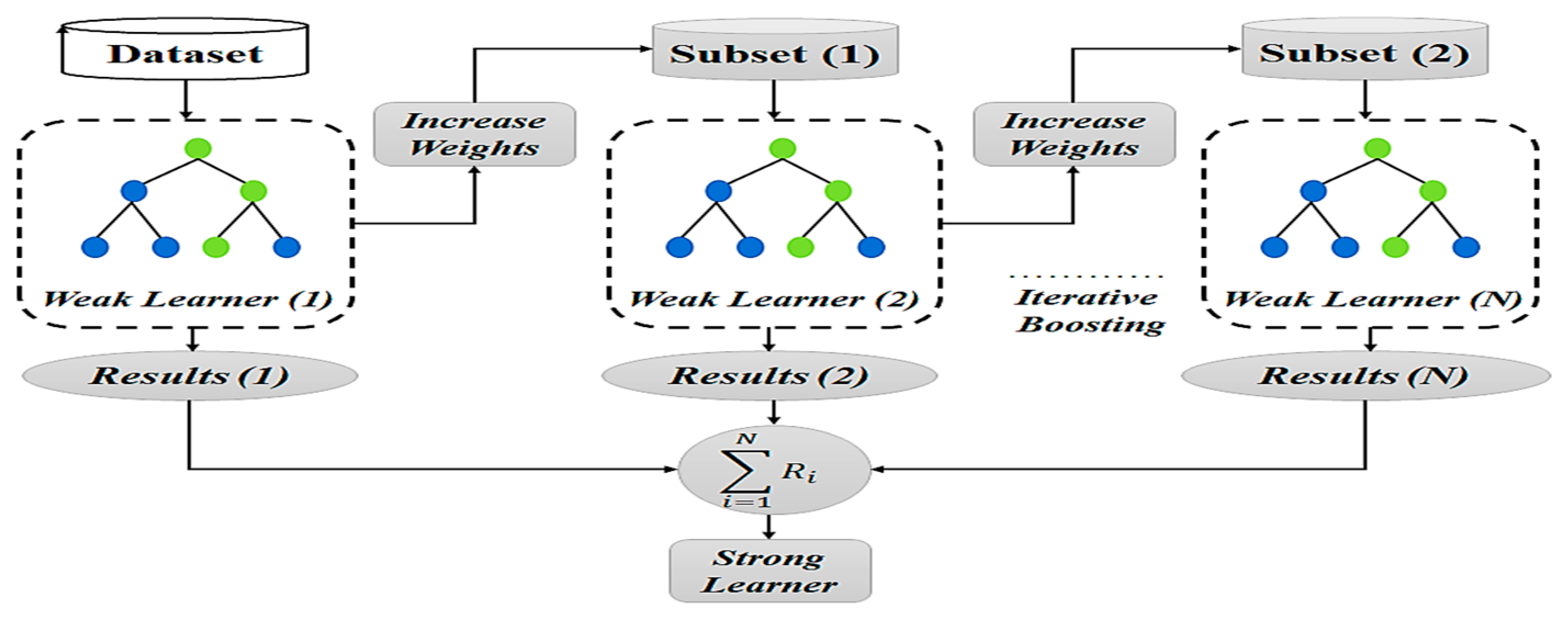
3.1.3. Gradient Boosting Classifier

GBC periodically introduces weak learners to minimise the loss function. At every iteration (n), a new tree is fitted to the negative gradient of the loss function that was calculated using the output from the previous ensemble as shown in Figure 4. While XGBoost includes regularisation and optimisation at the system level, GBC is a more classical implementation [21]. The prediction by GBC can be calculated as follows:

$$F_n\left(\mathrm{x}\right)=F_{n-1 }\left(\mathrm{x}\right)+\gamma h_n\left(\mathrm{x}\right)$$

(9)

where the cumulative prediction from the previous iteration is represented by $F_{n-1}$(x). The new weak learner is $h_n$(x). The learning rate γ regulates the new learner’s contribution. After learning to minimise the loss function, the weak learner $h_n$(x) can be calculated as follows.

$$h_n\left(\mathrm{x}\right)=\mathit{arg} {min}_h{\sum }_{i=1}^{n}l (y_i, F_{n-1}\left(x_i\right)+h (x_i))$$

(10)

The iterative error-correction process of the GBC makes it a great option for identifying hidden patterns in student behaviour. GBC is exceptionally effective at modelling complex relationships between variables, such as success, mistakes, and dropout, since each tree focuses on fixing the errors made by the earlier ones [21]. It may be modified for binary classification tasks due to its flexibility in handling different loss functions, and its ability to represent feature interactions offers a greater awareness of dropout risks.

3.1.4. Extreme Gradient Boosting

A gradient boosting algorithm known as XGBoost optimises an objective function that consists of a regularisation term and a loss term [22]. Decision trees are constructed in order, with each tree fixing the mistakes of the one before it. The following is a calculation for the XGBoost objective function:

$$O{F }_{XGB}(\theta )={\sum }_{i=1}^{n}l(y_i, {\widehat{y}}_i)+ {\sum }_{k=1}^k\mathsf{\Omega }\left(f_k\right)$$

(11)

where the loss function is denoted by $(y_i,{\widehat{y}}_i)$, and Ω($f_k$) represents the regularisation term for the k-th tree and can be calculated as follows:

$$\Omega \left(f_k\right)=\gamma T+{\displaystyle \frac{1}{2}}\lambda {\left|w\right|}^2$$

(12)

In Equation (12), T represents the number of leaves in the tree. The symbol λ is the L2 regularisation parameter for leaf weights ($w$). And γ denotes the complexity penalty controls [22]. The prediction ${\widehat{y}}_i$ at iteration t depends on the output of the t-th tree $f_t$($x_i)$, and can be calculated as follows.

$${\widehat{y}}_i^{\left(t\right)}={\widehat{y}}_i^{(t-1)}+f_t\left(x_i\right)$$

(13)

The second-order gradients are used by the XGBoost to effectively optimise the objective function. Equation (14) uses regularisation terms and second-order gradients of the loss function to quantify the XGBoost split improvement in the loss function as a gain [23].

$$G_{LF}={\displaystyle \frac{1}{2}}\left[{\displaystyle \frac{{\left(\sum G_j\right)}^2}{\sum H_j+\lambda }}-{\displaystyle \frac{{\left(\sum G_L\right)}^2}{\sum H_L+\lambda }}-{\displaystyle \frac{{\left(\sum G_R\right)}^2}{\sum H_R+\lambda }}\right]-\gamma$$

(14)

where the first and second derivatives of the loss function for the j-th instance are denoted by $G_j$ and $H_j$. For every instance in the left subset of the data split, the first- and second-order gradients are denoted by $G_L$ and $H_L$. And for the data split, $G_R$, $H_R$ represent the right subset of data. The regularisation parameter γ regulates the smallest loss improvement necessary for a split to take place [23]. The symbol γ serves as a threshold, while a split is not used if its split gain is smaller than the threshold.

By avoiding splits that do not significantly improve model performance, XGBoost helps prevent overfitting. Additionally, by prioritising the most informative features, such as dropout probabilities derived from earlier sentences, XGBoost calculates the gain for each split, ensuring that only the most relevant features contribute to decisions of the model [22,23].

3.2. The Meta Model

The meta-learner of the stacked ensemble framework is implemented using an MLP, which is a sort of feed-forward neural network. The MLP is the last decision-making layer, integrating the base learners’ predictions with the original features to obtain the final output [24]. The meta-learner functions as a higher-level model, learning to combine the base models’ outputs into a single prediction. The MLP captures nonlinear relationships between meta-feature base model predictions and original features by using base models [25].

An MLP consists of multiple layers of neurons, input, hidden, and output layers, with each neuron performing a weighted sum followed by an activation function [25]. The input to the MLP is a vector X ϵ $R^d$, where d is the dimensionality of the enhanced feature set, and X is equal to [$x_1$, $x_2$, ……… $x_d$]. Each hidden layer transforms the input using trainable weights $w^{\left(l\right)}$ and biases $b^{\left(l\right)}$ [24,25]. The output of the $l$-th layer is calculated as shown below.

$$h^{\left(l\right)}=\mathsf{\sigma } (w^{\left(l\right)}{h}^{(l-1)}+b^{\left(l\right)})$$

(15)

The output of the previous layer is denoted by $h^{(l-1)}$. Weight matrix and bias vector for the $l$-th layer represented by $w^{\left(l\right)}$ and $b^{\left(l\right)}$, respectively. σ is an activation function [26]. The output prediction $\widehat{y}$ is generated by the last layer and is computed as follows:

$$\widehat{y}=\mathit{ReLU} (w^{\left(l\right)}{h}^{(l-1)}+b^{\left(l\right)})$$

(16)

The expression for the Rectified Linear Unit (ReLU) activation function is σ(x) = max (0, x). Back propagation is used to train the MLP by minimising a loss function [24]. The difference between the true labels y and the predicted probability $\widehat{y}$ for the i-th sample measured by the loss function is as follows [27].

$$L(y, \widehat{y})=-{\displaystyle \frac{1}{N}}{\sum }_{i=1}^N{[y}_i{\mathit{log}(\widehat{y}}_i)+\left(1-y_i\right)\mathit{log}(1-{\widehat{y}}_i)]$$

(17)

where N is the number of training samples. Gradient descent is used to iteratively adjust the weights $w^{\left(l\right)}$ and biases $b^{\left(l\right)}$ during training, which are calculated as follows.

$$w^{\left(l\right)}=w^{\left(l\right)}-\eta {\displaystyle \frac{\partial L}{\partial w^{\left(l\right)} }}$$

(18)

$$b^{\left(l\right)}=b^{\left(l\right)}-\eta {\displaystyle \frac{\partial L}{\partial b^{\left(l\right)} }}$$

(19)

In Equations (18) and (19), η represents the learning rate, and ${\displaystyle \frac{\partial \mathrm{L}}{\partial w^{\left(l\right)}}}$ and ${\displaystyle \frac{\partial \mathrm{L}}{\partial b^{\left(l\right)}}}$ are the gradients of the loss concerning the weights and biases. By improving the outputs of the basic model and minimising overfitting using regularisation strategies, such as L2 regularisation, MLP makes it possible to increase the ability of the ensemble to generalise to new data [27].

3.3. Grid Search Cross-Validation

A crucial step in maximising the performance of ML models is hyperparameter tuning. Selecting the ideal combination that maximises or minimises a performance metric, including accuracy, precision, and recall, requires searching through a predetermined set of hyperparameters [28]. Identifying the ideal hyperparameter combination that optimises the performance score across all folds in k-fold cross-validation is made possible by grid search cross-validation (Grid Search CV). The following equation can be used to find the best hyperparameter combination:

$${\theta }^{\mathrm{*}}=\mathit{arg} {max}_{\mathsf{\theta }\mathsf{ϵ}\mathsf{\delta }}{\displaystyle \frac{1}{k}}{\sum }_{i=1}^k{A}_i\left(\theta \right)$$

(20)

where δ represents the collection of every possible combination of hyperparameters. θ is a particular combination from δ. When using k-fold cross-validation, K is the number of folds. Additionally, the average performance score for all k folds is $A_i\left(\mathsf{\theta }\right)$. Grid Search CV is used to hyperparameter-tune both base and meta-learner models, such as for dropout prediction [29]. The combination objective for each model is calculated as follows:

$${\theta }^{\mathrm{*}} =\mathit{arg} {max}_{\mathsf{\theta }\mathsf{ϵ}\mathsf{\Theta }}{\displaystyle \frac{1}{k}}{\sum }_{i=1}^{k}accuracy(y_{t,i}, y_{p,i})$$

(21)

where $y_{t,i}$ and $y_{p,i}$ represent the true and predicted labels for the i-th fold. Grid Search CV makes it possible to identify the best hyperparameters for ML models. Reliable results are ensured by the evaluation of performance metrics throughout k folds of the method [29].

4. The Methodology

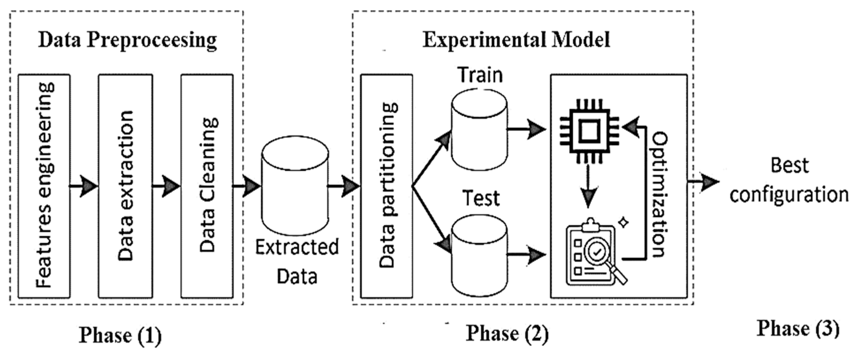
This study aims to predict the probability of student dropout using an in-session dataset. Unlike previous approaches, it adopts a finer-grained prediction strategy by re-estimating the dropout risk after each sentence submitted by the learner. With every new sentence, all previously submitted responses are used to update the prediction model. This incremental learning process allows the model to dynamically adapt to changes in learner behaviour throughout the session. As illustrated in Figure 5, the evaluation of the proposed approach is structured around three key methodological phases.

In-session databases do not directly support the use of learner data for predictive modelling. Therefore, a preprocessing step is required to transform the large volume of unstructured data into a structured format suitable for dropout prediction. This stage involves the use of a Python-based tool version 3.8, with the hardware and software specifications detailed in

Table 2. System specifications.

Hardware and Software	Specifications
CPU	x64 built on 20240913, e2-custom-6-49152 (6 vCPUs)
RAM	48 GB
Operating system	Windows Server 2019
virtual machine (VM)	Google VM

. The resulting dataset captures both individual session activities and cumulative behavioural patterns over time, generated from aggregated user interaction data using predictive features related to learner engagement.

4.1. Data Collection and Preprocessing

The dataset used in this study is obtained from this link, (https://zenodo.org/records/7755363 (accessed on 6 June 2024)), which is a real-world online language learning platform that offers interactive grammar, spelling, and punctuation tasks. The information includes recorded student interactions for a total of 52,032 students, 164,580 sessions, and 3,224,014 phrases turned in for 181,792 assignments. Up to ten sentences are taken from exercises included in each session, and each submission is recorded as a distinct instance in the dataset [30]. Sentence-level dropout prediction is made possible by this structure, which also enables the model to constantly update risk ratings following each interaction. Because of this degree of detail, the dataset is especially well-suited for real-time educational analytics and enables in-session intervention methods.

The selected time frame of the dataset is from March to April 2020 that corresponds to a typical mid-academic-year period, ensuring that the dataset reflects normal learning behaviour without being influenced by end-of-term anomalies or special interventions. It captures both voluntary and mandatory learner engagement, offering a representative sample of diverse learning motivations and behavioural patterns. This dataset has been used in prior studies related to learner engagement and performance modelling, confirming its validity and relevance in educational data mining tasks [11].

The in-session dataset includes a wide range of variables related to student performance and behaviour. Each row in the dataset corresponds to a specific sentence in the course progression, represented by a unique matrix value. The target variable, dropout, is binary, indicating whether a student left the session or remained engaged. Before modelling, several preprocessing steps were applied to clean and prepare the data.

▪

Removal of redundant identifiers: Columns such as index, ID, and session ID were removed, as they do not contribute to the predictive capability of the model and may introduce noise.

▪

Segmentation by sentence position: The dataset was divided into smaller subsets based on the matrix column, which denotes the position of each sentence within a session. This matrix value ranges from 1 to 300, representing each specific sentence submitted by a student.

▪

Feature selection: A predefined set of high-performing features was selected using empirical analysis and domain knowledge. These features capture various aspects of learner engagement and performance.

The data was cleaned to ensure the quality of the dataset before training the model. Two key aspects of the process involved handling missing values and outliers. During the initial exploratory data analysis, some features were identified as having missing or empty entries, particularly in fields related to user attributes and test participation. These were due to optional fields or incomplete session records [31]. For numerical features, missing values were imputed using the mean value of the feature, as it is less sensitive to outliers than the mean. For binary features, missing values were replaced with 0 based on context and domain knowledge. In cases where more than 70% of values were missing in a feature across all learners, the feature was dropped from the final dataset to avoid introducing bias or noise.

Several numerical outliers, including steps, failures, and accomplishments, had variances recorded. Steps and errors were examples of qualities that maintained extreme but believable actions. Outliers were inputs that were obviously invalid, like time values that were negative [31]. Z-score normalisation was applied to scale numerical features, reducing the influence of extreme values without losing meaningful variance.

In the preprocessing stage, up to 60 matrices were made for each user to ensure scalability and relevance. As more data becomes available, this approach enables the predictive model to expand gradually, capturing both short-term and long-term behavioural trends. The raw data was processed to identify significant variables that reflect performance and engagement to successfully model learner behaviour. The data of every learner and every sentence in a session served as a basis for creating the usable dataset [30,31]. The learner’s behaviour during a specific sentence S is represented as a vector ($L_S$).

$$L_S=\{L_a^S, L_b^S, \dots \dots L_p^S\}$$

(22)

where the sentence position within the session is indicated by the S index. P indicates the total number of predictive features. The cumulative behaviour from earlier sentences was combined with the present sentence’s vector ($L_S$) to take into consideration temporal dynamics in learner behaviour [30]. The following is the cumulative representation ($C_i$) of a learner’s actions up to sentence i, which depends on the learner’s behaviour ($L_i$):

$$C_i=C_{i-1}+L_i$$

(23)

In Equation (22), $C_{i-1}$ represents the cumulative representation of learner behaviour for the previous sentence. With each additional sentence that is submitted, the dataset grows incrementally since the matrix value indicates the sentence location inside the session [31]. The model only utilises the first sentence to generate predictions at the start of the session. As the session continues, the model adds more sentences and updates its predictions according to the learner’s cumulative behaviour. This method makes sure that the model adjusts dynamically to variations in learner behaviour by methodically combining sentence-level data and recalculating predictions following each phrase.

Class imbalance, in which there are many more non-dropout cases than dropout instances, is a common problem in dropout prediction tasks. Random under-sampling (RUS) was used to solve this problem [31]. Although under-sampling may result in information loss, it ensures that the model is trained on a balanced dataset, which enhances its capacity to forecast dropouts from minority classes. Since the number of non-dropouts generally significantly outnumbers dropouts in in-session datasets, which naturally reflects class imbalance, using RUS in the preprocessing phase helped balance the class distribution. This step enhanced the model’s ability to identify at-risk learners and prevented it from being biased toward the majority class.

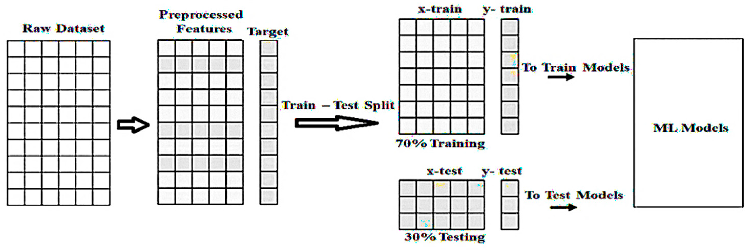
4.2. The Proposed ISELDP Model

In the proposed In-session Stacked Ensemble Learning for Dropout Prediction (ISELDP) framework, two essential steps are involved in building a predictive model using machine learning algorithms: training and testing. The dataset is split such that 70% is used for training—ensuring the model can generalise effectively across diverse learner profiles and avoid issues such as underfitting—while the remaining 30% is reserved for testing. To preserve the class distribution of the target variable (dropout), the split is performed using stratified sampling. The experimental framework for dropout prediction is illustrated in Figure 6.

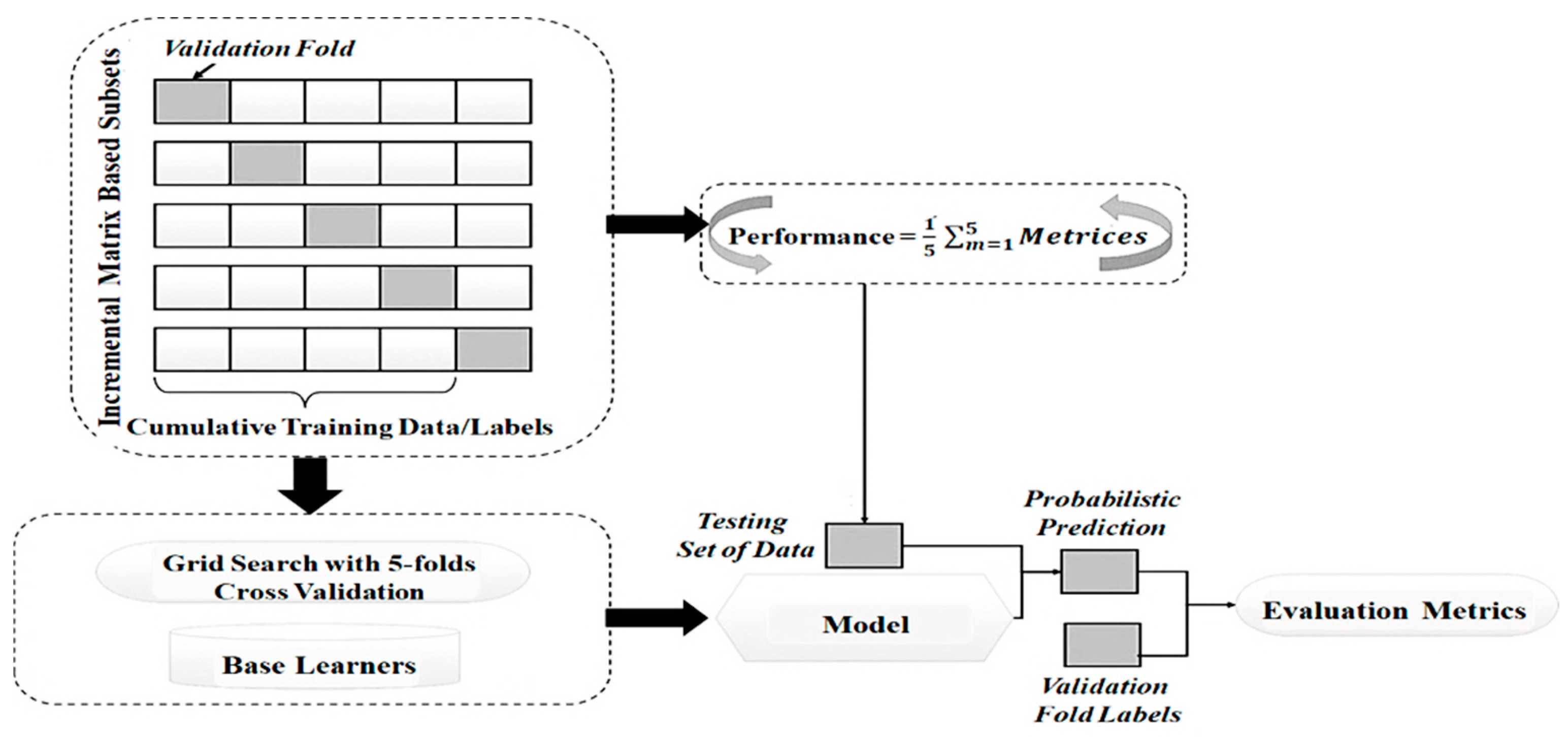
To train the meta-learner, implemented as an MLP, the modelling phase adopts an ensemble approach that integrates the predictions of four base models: AdaBoost, RF, XGBoost, and GBC. To optimise the performance of all models, Grid Search CV, as illustrated in Figure 7, is employed for hyperparameter tuning.

AdaBoost, RF, XGBoost, and GBC are the four basis classifiers that have been selected because of their complimentary abilities to handle noisy and unbalanced data, which is typical of in-session datasets. AdaBoost is excellent at focusing on hard-to-classify cases, XGBoost has significant regularisation capabilities, RF provides robustness through ensemble averages, and GBC, with careful adjustment, provides high predicted accuracy [31]. Because of its flexibility in learning complex decision limits from the basic models’ outputs, the MLP meta-learner was selected.

The MLP meta-learner is designed with four hidden layers of decreasing sizes (35, 28, 17, and 9 neurons, respectively), reflecting a gradual reduction in dimensionality across layers. This architectural choice enhances the ability of the model to generalise by enabling it to learn hierarchical representations of the input features [31,32]. The process of the proposed stacking model is outlined in Algorithm 1.

Algorithm 1: ISELDP Model for In-session dropout prediction

Input: Dataset D, Number of matrix values M, Feature subset F data collection from dataset Output: Trained stacking model S Preprocessing: Load dataset D and assign column names Drop the irrelevant columns index, session ID Identify unique matrix values {$M_1$, $M_2$,…, $M_m$}. Initialise storage for metrics (F1-Score, AUC, Accuracy, precision, Recall, MCC) for each matrix value m from 1 to M do    Extract subset $D_m$ corresponding to matrix value m.     if m > 1 then     Concatenate $D_m$ with previous data to form a cumulative dataset $D_{cum}$     else     Set $D_{cum}$ = $D_m$     end if Class Balancing (Under-Sampling):     Separate the independent variable X and the dependent variable y from $D_{cum}$     Apply RUS to balance classes in X and Y Feature Selection:     Select features using hardcoded indices F     Update X to include only selected features     Split X and y into 70% training ($X_{trian}$, $y_{trian}$) and 30% testing ($X_{test}$, $y_{test}$) sets Base Learner Prediction:     Initialise base learners: AdaBoost ($B_1$), RF ($B_2$), XGBoost ($B_3$), GBC ($B_4$).     for each base learner $B_i$ in {$B_1$,$B_2$,$B_3$,$B_4$} do     Perform Grid Search to tune hyperparameters of $B_i$ on $X_{trian }$ and $y_{trian }$        Train tuned $B_i$ on $X_{trian }$        Generate predictions $P_{train}^i$ and $P_{test}^i$ for $X_{trian }$ and $y_{trian }$     Combine $P_{train}^i$ and $P_{test}^i$ across all base learners into matrices $P_{trian }$ and $P_{test }$     Append $P_{trian}$ and $P_{test }$ to original features $X_{trian }$, and $X_{test}$ to form meta datasets.     end for Meta-Learner Prediction and Evaluation:      Initialise MLP meta-learner M      Repeat step (23) for meta-learner M on $P_{trian }$ and $y_{trian }$      Repeat Step (24) for tuned M on $P_{trian }$      Generate predictions ${\widehat{y}}_{test}$ for $P_{test }$     Compute evaluation metrics using ${\widehat{y}}_{test}$ and $y_{test }$ end for Get meta model Prediction $M_k$ Final predictions $M_k$

As shown in Figure 7, Grid Search with 5-fold cross-validation is used to perform hyperparameter tuning for the stacking process. This involves training four base learners, whose probabilistic predictions are then used as input to train the MLP meta-learner. To ensure effective training and address the issue of vanishing gradients, the MLP employs ReLU activation functions in its hidden layers. This architecture facilitates the detection of complex data patterns while reducing the risk of overfitting by progressively decreasing the number of neurons across layers [32].

The weights of the model are optimised using the Adam optimiser, which provides stable convergence and adaptability to the data. Additionally, early stopping is implemented to halt training when the validation performance no longer improves, further reducing the risk of overfitting [32]. This hierarchical structure enables the meta-learner to harness the strengths of diverse base models while compensating for their individual limitations.

Since ISELDP employs sentence-level incremental modelling, updating predictions after each sentence input, the final evaluation used a cumulative dropout approach combined with GridSearchCV and stratified 5-fold cross-validation to optimise the hyperparameters of each base model. An accumulated dataset of all prior sentences was used to train the model at each matrix value representing sentence position. Prediction conditions were simulated at each stage using a fixed 70–30 train–test split.

4.3. Model Configuration and Experimental Metrics

The design of the dropout prediction framework emphasises performance optimisation through systematic model configuration and hyperparameter tuning. Four machine learning methods were selected as base models due to their effectiveness in handling classification tasks involving high-dimensional and complex in-session data. To avoid the imbalance of early matrix values during the time evolution of session data and prediction at the first sentences, RUS is used at all sentences levels to ensure that the model can efficiently learn from dropout and non-dropout cases throughout the session. The meta-learner combines both the original features and the predictions from these base models.

Table 3. The ML models’ parameters.

Parameters	Models	Values
Number of estimators	RF	50, 100, 150
	AdaBoost
	GBC
	XGBoost
Max learning rate	RF	0.2
	AdaBoost	1
	GBC	0.2
	XGBoost	0.3
Max depth	RF	10
	GBC	3, 5, 7
	XGBoost
Alpha (regularisation)	MLP	0.01, 0.0001
Activation function		ReLU
Max iterations		100

summarises the configuration parameters for all models used.

GridSearchCV was used for tuning hyperparameters using cross-validation. To balance model complexity and training duration, for instance, the number of estimators in models was adjusted between 50, 100, and 150. To avoid overfitting and maintain the expressiveness of the model, learning rates and maximum depths were adjusted within accepted bounds.

The performance of the proposed approach was evaluated using various metrics alongside the basic classifiers. Accuracy represents the percentage of correct predictions made by the model and is calculated as the number of accurate estimations divided by the total number of predictions [32]. Precision, also known as positive predictive value, is the ratio of relevant instances among the retrieved ones. Recall, or sensitivity, measures the proportion of relevant instances that were correctly identified. The F1-score is a harmonic mean of precision and recall, providing a balanced measure of a model’s performance. The Matthews Correlation Coefficient (MCC) evaluates the quality of binary or multiclass classifications by considering true and false positives and negatives.

Additionally, the Area Under the Receiver Operating Characteristic Curve (AUC) indicates the probability that the model ranks a randomly chosen positive instance higher than a randomly chosen negative one [33]. The formulas for calculating each metric are provided as follows.

$$\mathit{Precision}={\displaystyle \frac{TP}{TP+FP}}$$

(24)

$$\mathit{Recall}={\displaystyle \frac{TP}{TP+FN}}$$

(25)

$$\mathit{Accuracy}={\displaystyle \frac{TP+TN}{TP+TN+FN+FP}}$$

(26)

$$F1 \mathit{score}=2\times {\displaystyle \frac{Recall\times Precision}{Recall+Precision}}$$

(27)

$$MCC={\displaystyle \frac{\left(TP\times TN\right)-(FP\times FN)}{\sqrt{\left(TP+FP\right)(TP+FN)(TN+FP)(TN+FN)}}}$$

(28)

$$\mathrm{AUC} = {\int }_0^{1}Recall \left(FPR\right)d\left(FPR\right)$$

(29)

where the true positive (TP): correct positive prediction; false positive (FP): incorrect positive prediction; true negative (TN): correct negative prediction; false negative (FN): incorrect negative prediction; and FPR is the false positive rate given by FP/(FP + TN).

4.4. Methodological Limitations

There are a few limitations to the proposed ISELDP model, considering its excellent performance in predicting dropout during in-session learning. First, especially in the early parts of a session where dropout instances are rare, the use of RUS may lead to the loss of potentially relevant majority class examples. However, as more sentences are processed, RUS tends to better preserve these majority class instances. Second, other stacking concepts that might better capture temporal dependencies, like LR, are not as easily explored when used with MLP as a meta-learner. Lastly, the stacked ensemble’s complexity raises the possibility of overfitting, especially when training on little session data subsets. However, with more data subsets it provides an efficient performance.

Another consideration is related to the use of the RUS approach. While it makes the model more sensitive to dropout cases, it can also lead to the loss of instances from the majority class that could be useful, particularly in the early phases of session data when dropout events are uncommon. Nevertheless, despite these limitations, real-time in-session monitoring systems certainly stand to gain from ISELDP’s predictive abilities. The model allows early intervention methods like adaptive feedback, motivating indications when disengagement is detected by dynamically updating predictions after each sentence. It could be integrated into adaptive learning platforms due to its incremental architecture, which enables reactive instructional modifications in response to changing student behaviour [34].

5. Simulation Results and Discussion

This section evaluates and analyses the performance of the proposed approach in two phases. In the first phase, the general performance of the model is assessed under two data scenarios: imbalanced and balanced datasets. This evaluation highlights the model’s effectiveness in predicting student dropout. In the second phase, the proposed approach is compared with a benchmarking study to showcase its unique performance. With improved meta-learners, the results demonstrate the progress achieved through the use of a learning ensemble framework in this comprehensive assessment.

5.1. General Performance

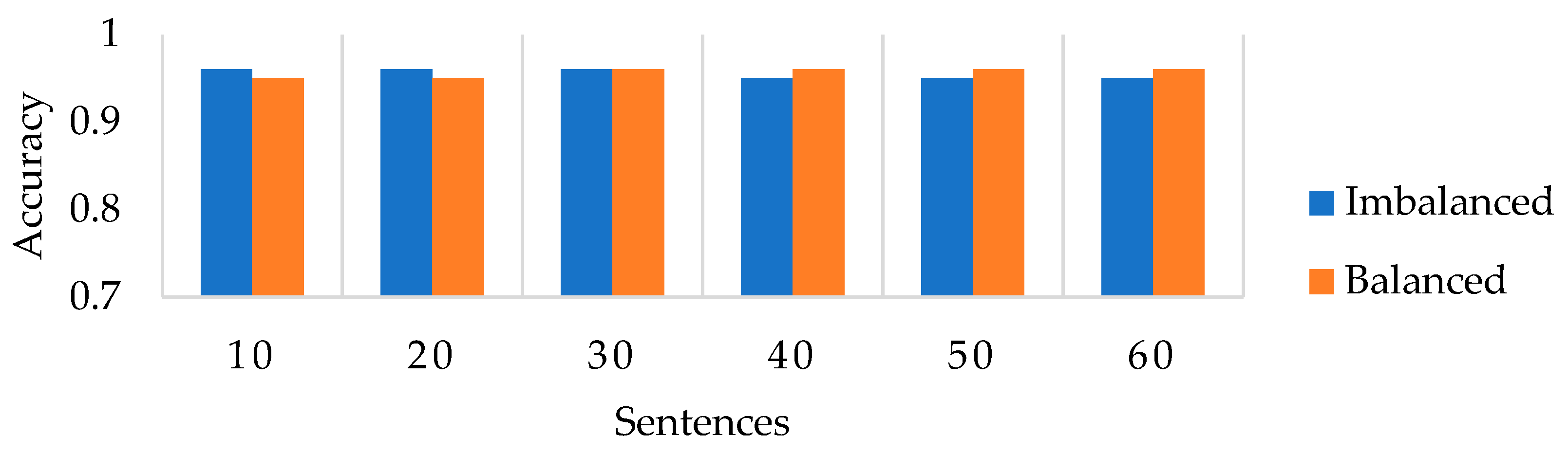
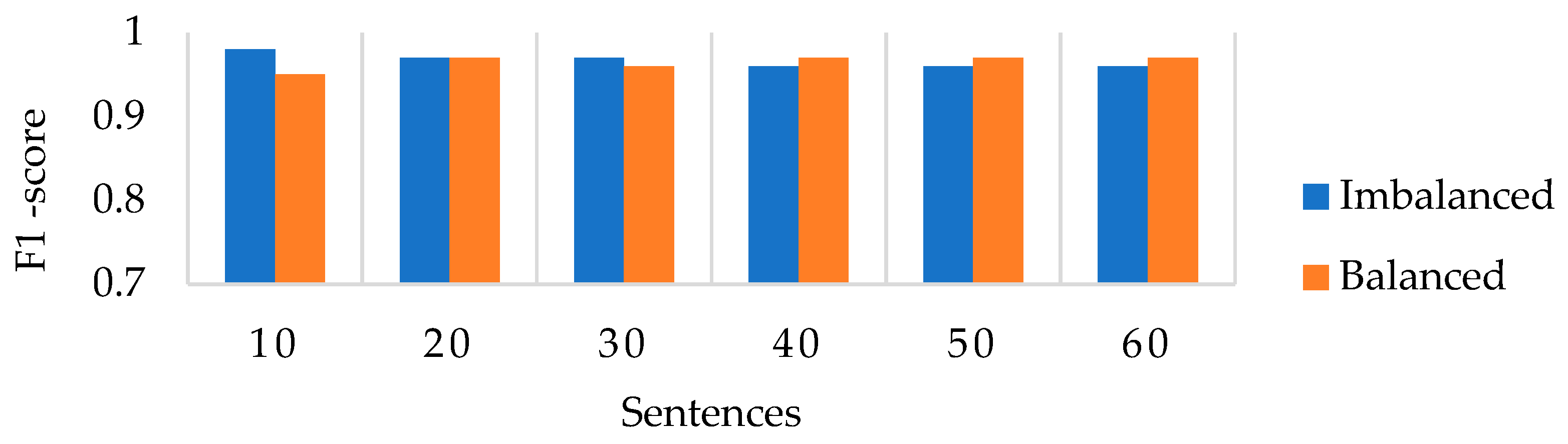
Figure 8 and Figure 9 present a comparison of the performance of the stacked ensemble’s meta-MLP model across two data scenarios: imbalanced and balanced datasets. Figure 8 specifically illustrates the prediction accuracy of the proposed stacked ensemble meta-MLP model in both scenarios. The model achieves high accuracy when trained on imbalanced data; however, this performance degrades as more test instances are introduced, although the accuracy still exceeds 92%. This outcome aligns with findings in the literature, which indicate that class imbalance tends to bias predictions toward the majority class, negatively impacting classification performance. Consequently, the model sensitivity to dropout events is reduced.

In contrast, when trained on balanced data, the proposed model shows significant improvement. Accuracy steadily increases, with an observed improvement of 1.2%. This indicates that balancing the dataset enhances the model’s ability to learn discriminative features for both dropout and non-dropout classes by ensuring fair representation during training. These results underscore the added value of using balanced data with a stacked ensemble model, which contributes to improved classification by reducing dimensionality and minimising the influence of underrepresented classes.

Figure 9 illustrates the F1-score performance of the stacked ensemble meta-MLP model. Notably, the imbalanced scenario initially performs slightly better than the balanced scenario, primarily due to higher recall for the non-dropout class, which benefits from its majority representation. However, this comes at the cost of reduced sensitivity to the minority (dropout) class and does not reflect a truly balanced performance.

In contrast, the balanced scenario shows slightly lower F1-scores during the early stages, possibly because the model requires more instances to fully leverage the balanced class distribution and extract refined features. From sentence 40 onward, the F1-scores of both scenarios begin to converge, with the balanced configuration consistently outperforming the imbalanced one in the later stages (sentences 40 to 60). This shift indicates that, once sufficient data is collected during a session, the balanced dataset enables the model to better capture relevant predictors.

The steady increase in F1-score under balanced conditions throughout the modelling process confirms the value of preprocessing techniques. These methods contribute to more stable and reliable performance, ultimately enhancing the model’s accuracy in predicting student dropout in educational platforms.

Table 4. Other performance evaluations for stacked ensemble approach.

Scenarios	Precision	Recall	MCC	ROC-AUC
Imbalanced	0.93	0.98	0.09	0.55
Balanced	0.99	0.78	0.78	0.88

compares the performance of the stacked ensemble meta-MLP model across two training scenarios using four key performance metrics: average precision, recall, the Matthews Correlation Coefficient (MCC), and ROC-AUC. The results reveal that each data scenario presents distinct trade-offs. In the imbalanced scenario, the model achieves a relatively high recall of 0.98; however, its precision (0.93), ROC-AUC (0.55), and MCC (0.09) are significantly lower. These results indicate poor overall reliability across different classes. This outcome underscores a well-known limitation of imbalanced datasets: high recall often stems from the model’s bias toward the majority class, accompanied by a diminished ability to accurately identify the minority (dropout) class. Consequently, this reduces both the robustness and fairness of the model’s performance.

On the other hand, the MCC (0.78) and ROC-AUC (0.88) scores were significantly improved in the balanced scenario, indicating more reliable and consistent classification across classes. However, the recall value decreased to 0.78, reflecting a more conservative strategy that sacrifices some sensitivity in favour of higher precision (up to 0.99) and balanced classification performance. These results demonstrate that balancing the dataset leads to a more robust and practical predictive model for in-session dropout detection in educational platforms.

As a final observation, it is noted that while the balanced scenario ultimately outperforms the imbalanced one, it exhibits slightly lower F1-scores during the early phases of session interactions, specifically when the number of sentences ranges from 1 to 20. This can be attributed to two main factors. First, learners typically submit only a small number of sentences at the beginning of a session, limiting the available behavioural data and making it difficult to differentiate early signs of disengagement from normal engagement patterns. Second, the application of RUS can lead to the loss of potentially valuable majority class instances, which may temporarily reduce the model’s generalisation capability, especially when training data is limited.

However, as the session progresses and more data is collected, the balanced model benefits from improved representation of the minority class. This leads to better precision–recall trade-offs and higher overall F1-scores starting around sentence 40. In in-session environments, where early predictions must be handled with care, and model confidence increases with accumulating behavioural information, this pattern underscores the importance of dynamic modelling.

5.2. Comparison with Benchmarking Models

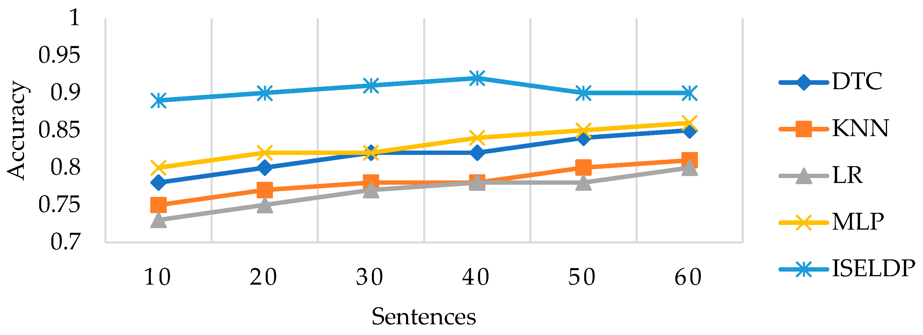
The accuracy and F1-score performance of the proposed ISELDP approach are compared with a benchmarking study using four machine learning models—Decision Tree Classifier (DTC), K-Nearest Neighbours (KNN), Logistic Regression (LR), and Multi-Layer Perceptron (MLP)—across six sentence-based assessment stages, as shown in Figure 10 and Figure 11. Figure 10 demonstrates that ISELDP maintains a consistently high performance throughout each sentence phase, with accuracy starting at 89% after 10 sentences and reaching 91% by sentence 40. These results highlight ISELDP’s ability to quickly adapt to user behaviour and improve its predictions as additional sequential data becomes available.

In contrast, the baseline models exhibit slower and more gradual improvements. KNN improves from 75% to 81%, and DTC increases from 77% to 85%, but both struggle to capture complex patterns in sequential learning activities, as shown by Nathalie et al. (2022) [11]. Although LR is computationally efficient, its accuracy remains relatively low, ranging from 71% to 79%, suggesting limited suitability for time-progressive dropout prediction tasks. MLP performs better than the other benchmark models, reaching 87% accuracy by sentence 60, yet still falls short of ISELDP’s performance.

These findings underscore the advantages of the ISELDP model, which integrates multiple base learners and leverages a meta-MLP to learn from their outputs. This ensemble design allows the model to benefit from diverse decision boundaries, improving both stability and generalisation. The notable increase in ISELDP’s accuracy after sentence 30 further demonstrates its capacity to effectively exploit temporal dependencies in learner behaviour. Overall, the model achieves an average accuracy of approximately 88% across all sentence stages, outperforming the benchmarking models.

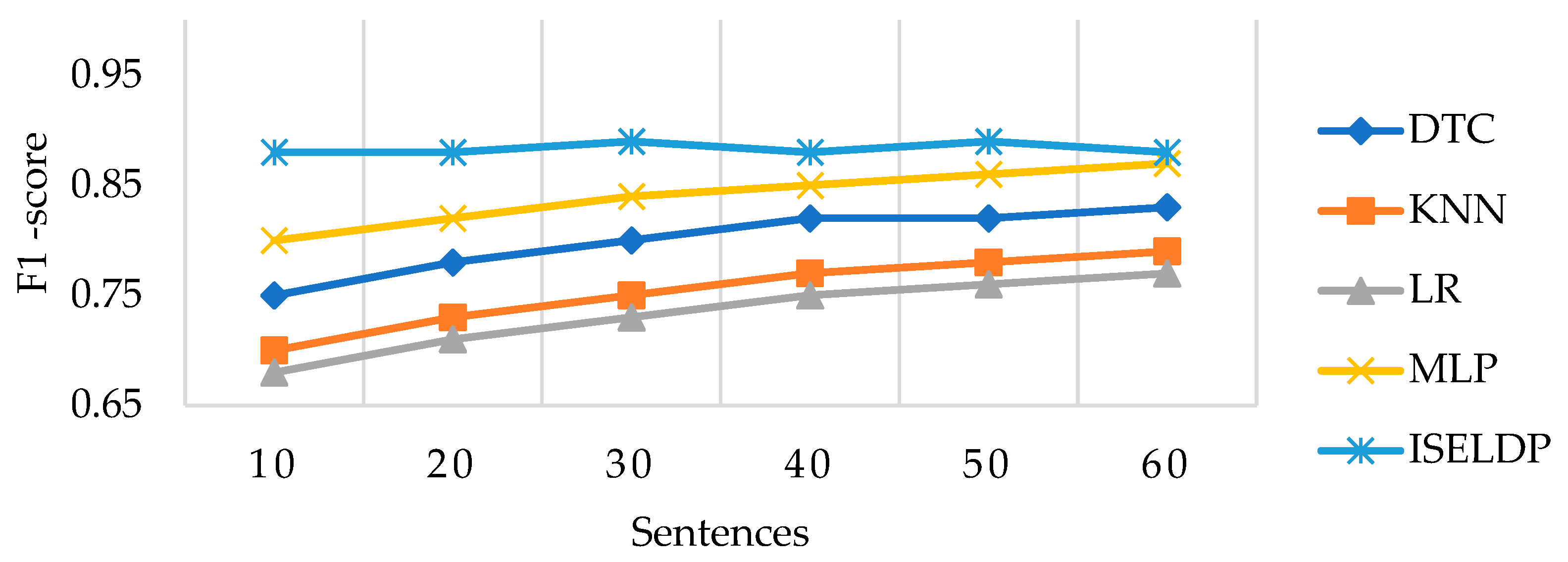
Figure 11 illustrates the superior classification balance achieved by the proposed ISELDP model compared to conventional benchmarking models, based on F1-scores across various sentence phases. The ISELDP model maintains consistently high F1-scores, reaching approximately 89% after just 10 sentences, briefly dipping to 88% around sentence 40, and then quickly recovering. This stability highlights ISELDP’s ability to effectively balance precision and recall, thereby enhancing the reliability of both early- and late-stage dropout predictions as sequential learning data evolves.

While the benchmarking models demonstrate gradual improvement, they consistently underperform compared to ISELDP. The DTC improves from 75% to 84%, showing modest gains but lacking the predictive robustness of the ensemble approach. KNN exhibits a steady increase from 70% to 80%, reflecting limited generalisation capabilities and a strong dependence on local data patterns. LR, constrained by its linear nature, performs the poorest, with F1-scores ranging between 67% and 76%, unable to capture complex learner behaviours as shown by [11]. Even though MLP achieves relatively higher F1-scores between 80% and 86% in the later stages, it still falls short of ISELDP, which achieves a near-optimal balance between false positives and false negatives.

These findings confirm that the ISELDP ensemble approach—featuring a high-capacity meta-level MLP and a diverse set of base classifiers—offers significant improvements in classification balance, especially in sentence phases where dropout prediction tends to be unbalanced. ISELDP demonstrates both rapid and stable performance convergence across sentence intervals.

Based on the results discussed, the ISELDP model clearly outperforms all baseline models, exhibiting consistent and superior predictive performance across all sentence thresholds. From sentence 40 onward, the model achieves peak accuracy and F1-scores of 88%, reflecting excellent classification precision and an optimal balance between sensitivity and specificity—two critical metrics for effective dropout detection in educational contexts. The stacked ensemble architecture, which leverages the strengths of multiple base learners and a meta-MLP, ensures robustness by improving generalisation, minimising individual model bias, and facilitating adaptability to classification errors. Furthermore, the model’s in-session prediction capability enables fine-grained temporal tracking, allowing dynamic adaptation to evolving learner behaviour patterns.

The results highlight the specific challenges in predicting dropouts during sessions, particularly in the early stages of interactions when the low dropout frequency may compromise model reliability. To improve the identification of the minority cases of dropouts and increase prediction accuracy in session datasets, the proposed approach uses incremental balancing. Additionally, using cost-effective learning methodologies and adaptive resampling approaches can enhance model performance in these unbalanced contexts, allowing for more precise and timely responses that are specific for each learner.

5.3. Computational Efficiency and Runtime Performance

The computational efficiency and latency of the proposed ISELDP model is evaluated in light of the in-session dropout prediction issue. The proposed model works under certain time limits because predictions are produced after every sentence.

Table 5. Performance of computation efficiency.

Metric	ISELDP (Stacked Ensemble)	MLP (Best Baseline)
Full training duration	7 days	6 h
Average training time per session	~30 min	~5 min
Inference latency per sentence	~25 ms	~8 ms
Memory footprint	~70 MB	~18 MB
CPU utilisation	~68%	~36%

shows the measured performance across experimental runs.

In Table 5, ISELDP’s inference time is under 100 ms, making it suitable for scenarios requiring immediate feedback after each interaction with the learner. While its training time is generally higher than that of single models, due to the use of multiple base learners and stacking, it remains acceptable for offline training contexts. The modest memory footprint of approximately 70 MB ensures compatibility with most modern web-based learning platforms without requiring complex hardware. Although the stacked ensemble incurs a higher computational cost compared to the MLP model, the roughly 2% improvement in prediction accuracy and 2.4% increase in balanced F1-score justify its use in environments where slight increases in latency are acceptable in exchange for better model performance.

6. Conclusions and Future Scope

The primary objective of this study was to develop a cumulative machine learning (ML) model, ISELDP, for predicting student dropout on educational learning platforms by analysing real-time interactions, where users and the platform exchange sentences. In-session datasets were selected as a suitable foundation due to the importance of features that reflect student behaviour. After preprocessing the data, relevant features were identified and analysed. A predictive model for student engagement was then constructed using AdaBoost, XGBoost, Random Forest (RF), and Gradient Boosting Classifier (GBC) as base learners. These algorithms, treated as weak learners, were subsequently integrated into a stacked ensemble model, with a Multi-Layer Perceptron (MLP) serving as the meta-learner.

The modelling results demonstrated that the proposed approach outperformed benchmarking techniques, particularly when trained on balanced data. The improvements can largely be attributed to the ensemble architecture, which combines multiple diverse base learners with an enhanced MLP, and to the effective use of the Random Under-Sampling (RUS) technique for addressing class imbalance. Furthermore, balancing the dataset and fine-tuning the MLP’s hyperparameters significantly improved the model’s generalisation and performance across evaluation metrics.

ISELDP represents an advanced solution in the domain of educational learning prediction due to its strong predictive capability and adaptability, particularly in dropout prediction tasks. To further improve the model’s accuracy, future work will focus on optimising the feature selection process. Currently, the model relies on hardcoded features, which limits its adaptability and may prevent it from dynamically identifying the most relevant attributes as data distributions evolve. Incorporating advanced feature selection techniques, such as genetic algorithms (GAs) combined with correlation-based feature selection (CFS), could help dynamically identify optimal feature subsets. These enhancements would not only improve model accuracy and generalisability but also increase computational efficiency by ensuring the model adapts more effectively to changing data patterns.