Abstract
Aiming at the problem of the through-core current sensor based on cable partial discharge detection having difficulty in compatibility with high sensitivity and wide detection frequency band, this paper proposes a design method for an ultra-high-frequency through-core current sensor. Firstly, the sensor circuit model was established, and the relationship between the sensor hardware parameters, and the bandwidth and sensitivity was derived. Subsequently, a multi-objective particle swarm optimization model was established. The sensitivity and bandwidth were taken as the objective functions, and the hardware parameters were regarded as the decision variables. Constraint conditions were set according to the cable size, self-integration working mode, etc. The optimal hardware parameters were obtained through solution and calculation. Finally, an ultra-high-frequency through-core current sensor was fabricated, and the bandwidth and sensitivity of the sensor at different frequencies were tested. The test results of cable partial discharge signals demonstrate that the designed sensor maintains a sensitivity of no less than 20.46 V/A within the 3 MHz to 200 MHz frequency range. This performance not only satisfies the fundamental sensitivity requirement of 5 V/A in the 3–30 MHz band for cable partial discharge detection but also resolves the inherent trade-off between sensitivity and detection bandwidth, exhibiting superior performance compared to conventional sensors.
1. Introduction
With the advancement of society, electricity has gradually become an indispensable component of human life. Power cables serve as the core medium for energy transmission in electrical systems. Although cable defects may not immediately lead to cable failure, prolonged operation can transform these defects into permanent faults, significantly compromising the reliability of power supply systems. Therefore, the timely detection of cable faults, precise localization of defects, and implementation of remedial measures are of critical importance for ensuring the stable operation of power grids [1].
Partial discharge detection and location are common means to discover cable insulation defects in a timely manner and ensure the safe operation of cables [2,3]. For cables in operation, to avoid economic losses caused by power outages, it is necessary to conduct online monitoring. State-of-the-art optical current sensors, while exhibiting exceptional dynamic response ranges, face practical limitations due to linear birefringence effects [4,5]. Graphene-based metamaterial sensors exhibit ultrahigh sensitivity yet require detection circuit reconfiguration and demonstrate nonlinear response characteristics due to resonant effects [6,7]. By contrast, the high-frequency current method is a commonly used and effective technique for partial discharge detection [8,9,10]. It does not need to establish a direct connection with the cable under test but rather couples a partial discharge signal at the grounding wire of the cable through the principle of electromagnetic induction. However, the energy of the partial discharge signal in the cable is relatively weak, typically in the range of several picocoulombs to several hundred picocoulombs, and its energy is distributed over a wide frequency band with high-frequency components. Therefore, the design of the through-hole current sensor is of vital importance [11]. Among them, the most common type of sensor is based on the principle of Roche coils, which has the advantages of simple manufacturing, ease of use, and wide application frequency band [12,13,14]. In recent years, there have been many studies on this through-hole current sensor. Jie Gong from Changsha University of Science and Technology derived the influence of the number of turns and the integrating resistance of the through-hole current sensor on the transmission impedance but did not consider the influence of the coil size [15]. The R. Giussani team developed sensors designed by grouping low and high frequencies, but the frequency band range of the high-frequency band used to collect partial discharge signals only reached 200 kHz–30 MHz [16]. However, the high-frequency component of the partial discharge signal of the cable can reach up to 100 MHz [17], which will lead to the inability to comprehensively obtain the fault information of the cable. The research team led by Qiaogen Zhang at Xi’an Jiaotong University developed a broadband current sensor with a frequency range of 800 kHz to 106 MHz; however, its limited sensitivity of merely 2.22 V/A [18] may result in the coupled signals being potentially obscured by noise.
In summary, existing through-core current sensors for partial discharge detection face the challenge of achieving both high sensitivity and wide detection bandwidth simultaneously. Furthermore, sensors employed for cable partial discharge monitoring must possess an adequately high upper cutoff frequency. To address these limitations, this study proposes the design of an Ultra-High-Frequency Current Transformer (UHFCT) based on the principles of electromagnetic induction and Rogowski coil. Through systematic optimization of hardware structural parameters, the developed UHFCT aims to meet the demanding requirements for cable partial discharge detection.
2. Current Sensor Model Establishment
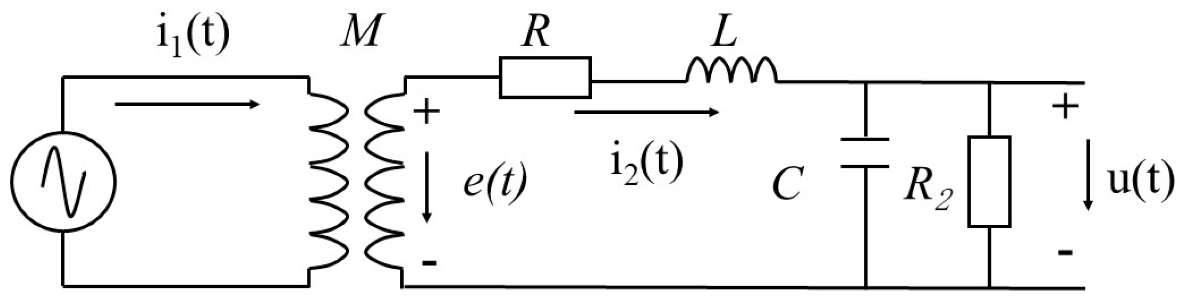
The Rogowski coil-type through-core current sensor operates based on Faraday’s law of electromagnetic induction. This sensor typically consists of a closed-loop coil and a pair of primary–secondary windings without electrical connections between them, with its structural configuration illustrated in Figure 1 [12]. The key design parameters include the inner radius rinside and outer radius routside of the toroidal coil, coil core thickness h, measured current i, sampling resistance R2, and output voltage U2. When a time-varying current flows through the current-carrying conductor perpendicular to the central axis of the coil former, the alternating magnetic field generated by the conductor induces a mutual inductance voltage across the coil. This induced voltage drives a current through the internal circuitry, ultimately producing an output voltage signal across the terminal resistor [19]. The equivalent circuit model is illustrated in Figure 2. In the equivalent circuit, M represents the mutual inductance between the primary and secondary sides, while R and L denote the internal resistance and self-inductance of the UHFCT, respectively, and C corresponds to the stray capacitance.
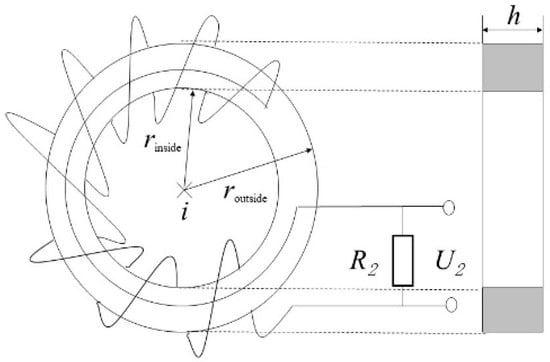
Figure 1.
Structure of Roche coil type through-core current sensor.

Figure 2.
Equivalent circuit model.
The electrical parameters in the equivalent circuit can be calculated using the following formulations:
In the formula, N is the number of turns of the winding coil; ρ and d are, respectively, the resistivity of the winding coil and the wire diameter; ε0 is the dielectric constant of vacuum; μ is the magnetic permeability.
Under self-integration conditions, where the distributed capacitance can be neglected, the loop voltage equation shown in Figure 2 yields:
The above expression can be simplified when either the product of the coil’s self-inductance and current change rate becomes sufficiently large or when the sampling resistance is sufficiently small:
The output voltage of the sampling resistor is:
Based on circuit theory, the transfer function of UHFCT can be obtained as follows, where U(s) and I(s) are the Laplace transforms of u(t) and i1(t), respectively.
Substituting s = j∗ω into the above equation yields:
Therefore, the amplitude–frequency characteristics of the current sensor are:
The upper and lower limit cutoff frequencies of the sensor can be calculated through the 3 dB principle [20,21,22]:
From this, the working frequency bandwidth can be obtained as:
Equation (13) reveals that the operational frequency bandwidth is determined collectively by the UHFCT’s internal resistance (R), self-inductance (L), stray capacitance (C), and output terminal resistance (R2).
Moreover, sensitivity represents a critical design consideration for coil sensors. The sensor exhibits band-pass frequency response characteristics, demonstrating higher sensitivity near its resonant frequency (ƒ0). At the operating frequency ω = ƒ0, the sensor’s sensitivity can be estimated as:
In summary, the sensitivity of the current sensor is jointly influenced by the number of coil turns (N) and the output terminal resistance (R2), while the bandwidth is collectively determined by the internal resistance (R), self-inductance (L), stray capacitance (C), and output resistance (R2). Increasing R2 to enhance sensitivity will result in bandwidth reduction. Similarly, reducing the number of turns (N) to improve sensitivity leads to increased inductance and internal resistance, which may also cause bandwidth degradation. Consequently, it is challenging to simultaneously achieve both high sensitivity and wide frequency bandwidth. To obtain optimal performance parameters, the following analysis will employ a controlled-variable approach to comprehensively evaluate the influence of various hardware parameters on sensor performance based on the established relationship between the equivalent circuit model parameters and the sensor’s physical characteristics.
3. Research on the Influence of Hardware Parameters on Sensor Performance
3.1. Magnetic Core Material
The characteristic parameters of common magnetic core materials are summarized in Table 1 [23].

Table 1.
Core material performance parameters.
This design specifically targets cable partial discharge detection, where the discharge signals exhibit a frequency spectrum extending up to hundreds of MHz [17]. Comparative analysis reveals that Ni-Zn ferrite cores demonstrate superior performance among the four material types, offering both higher cutoff frequency and lower high-frequency losses [24]. To optimize the UHFCT’s sensitivity and operational bandwidth while meeting all critical specifications, Ni-Zn ferrite was selected as the preferred magnetic core material [25].
3.2. Influence of Structural Parameters on Performance
Based on the model established in Section 2, the simulation results of the sensor performance were obtained by using the control variable method and successively changing the number of coil turns, wire diameter, inner and outer radii of the coil, thickness, and sampling resistance. By simulating the frequency characteristic curves of the sensor under different structural parameters, the influence degree and direction of the changes of each structural parameter on the frequency domain response and sensitivity can be visually observed.
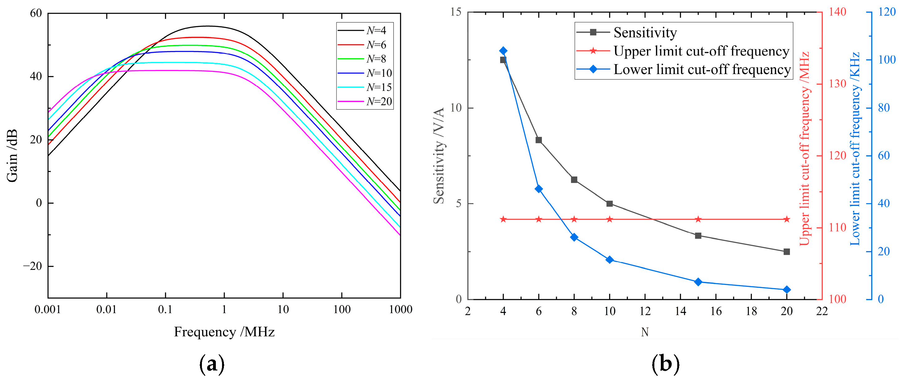
The simulation results of the turn influence on sensor performance are shown in Figure 3. The curves indicate that as the number of turns increases from 4 to 20, the upper cutoff frequency remains nearly unchanged, while the sensitivity decreases from 12.5 V/A to 2.5 V/A, and the lower cutoff frequency reduces from 103.95 kHz to 4.17 kHz. The frequency response curves exhibit a leftward shift with decreased peak values, showing an overall increasing trend in bandwidth.
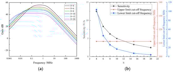
Figure 3.
(a) The influence of turns on amplitude–frequency characteristics. (b) The influence of turns on performance indicators.
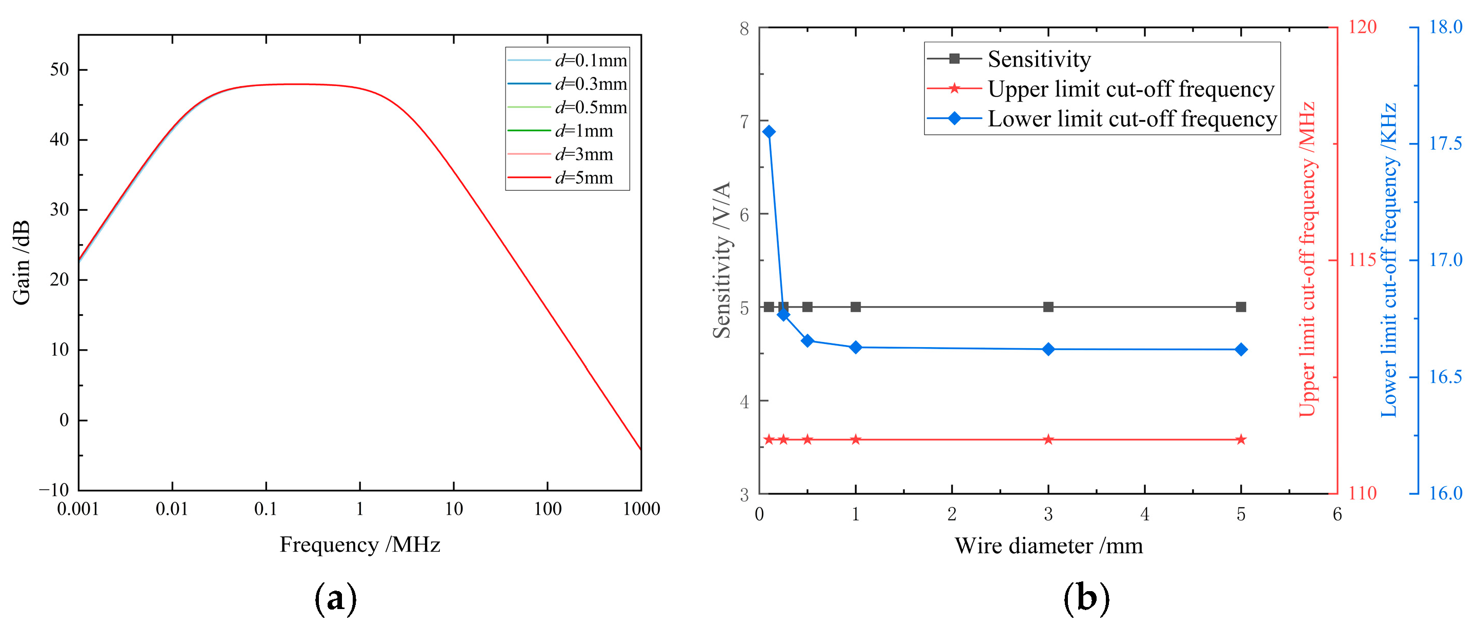
The simulation results demonstrating the impact of wire diameter variation on sensor performance are presented in Figure 4. The curves reveal that as the wire diameter increases from 0.1 mm to 5 mm, neither the cutoff frequency nor the sensitivity shows significant variation, with the frequency response remaining virtually unchanged. Since the actual variation range of wire diameter is limited in practice, the modification in wire diameter has negligible influence on both the bandwidth and sensitivity of the frequency response.
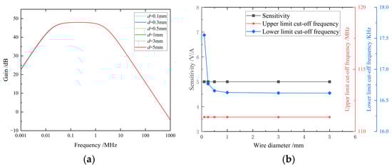
Figure 4.
(a) The influence of wire diameter on amplitude–frequency characteristics. (b) The influence of wire diameter on performance indicators.
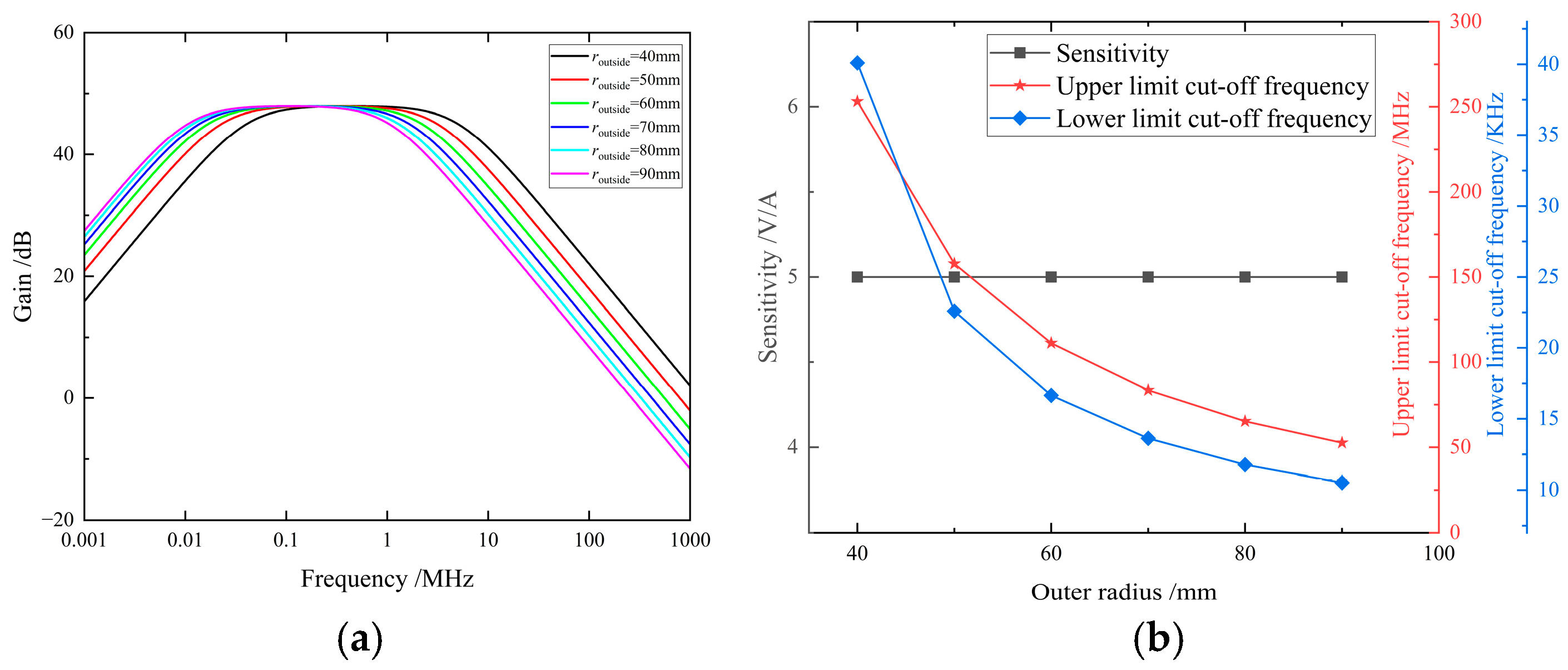
The simulation results demonstrating the impact of outer radius variation on sensor performance are presented in Figure 5. The curves reveal that as the outer radius increases from 40 mm to 90 mm, the sensitivity of the sensor is hardly affected, while the upper cutoff frequency decreases from 253.15 MHz to 52.06 MHz, and the lower cutoff frequency reduces from 40.1 kHz to 10.52 kHz. The frequency response curves exhibit a leftward shift, showing an overall decreasing trend in bandwidth.
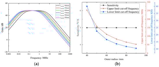
Figure 5.
(a) The influence of the outer radius of the coil on the amplitude–frequency characteristics. (b) The influence of the outer radius of the coil on the performance indicators.
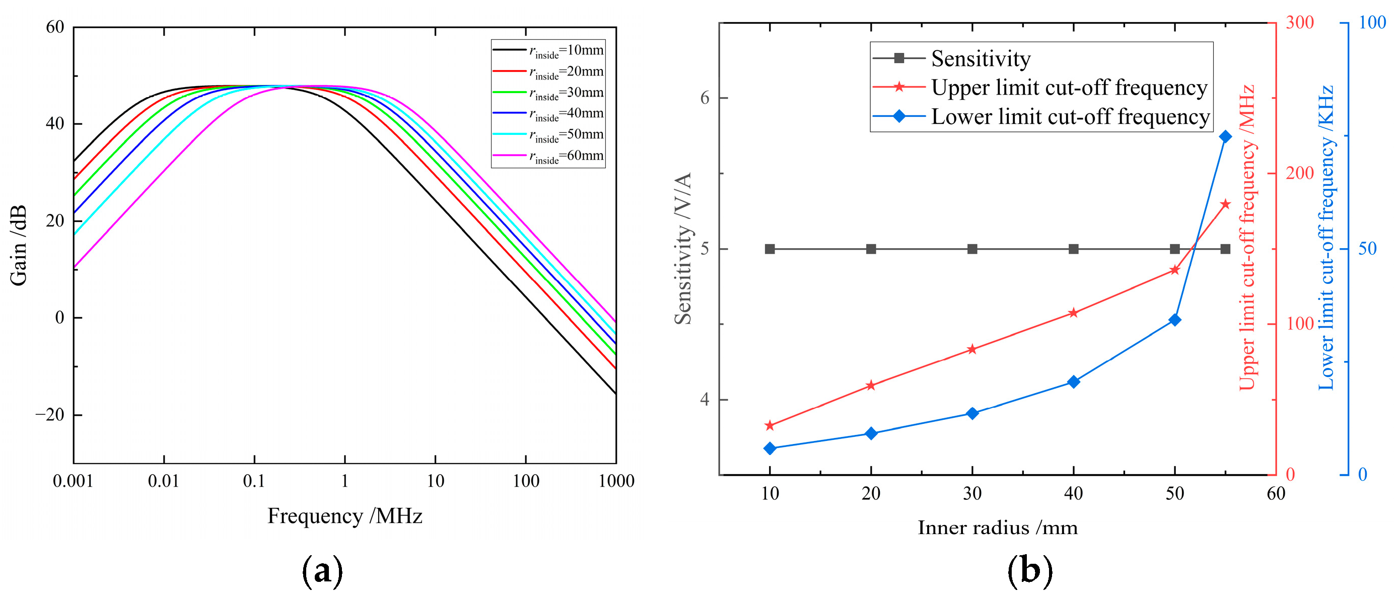
The simulation results of the inner radius’s influence on sensor performance are shown in Figure 6. The curves indicate that as the inner radius increases from 10 mm to 60 mm, the sensitivity of the sensor is hardly affected, while the upper cutoff frequency increases from 32.75 MHz to 179.67 MHz, and the lower cutoff frequency rises from 5.94 kHz to 74.84 kHz. The frequency response curves exhibit a rightward shift, with an overall increasing trend in bandwidth.
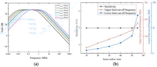
Figure 6.
(a) The influence of the inner radius of the coil on the amplitude–frequency characteristics. (b) The influence of the inner radius of the coil on the performance indicators.
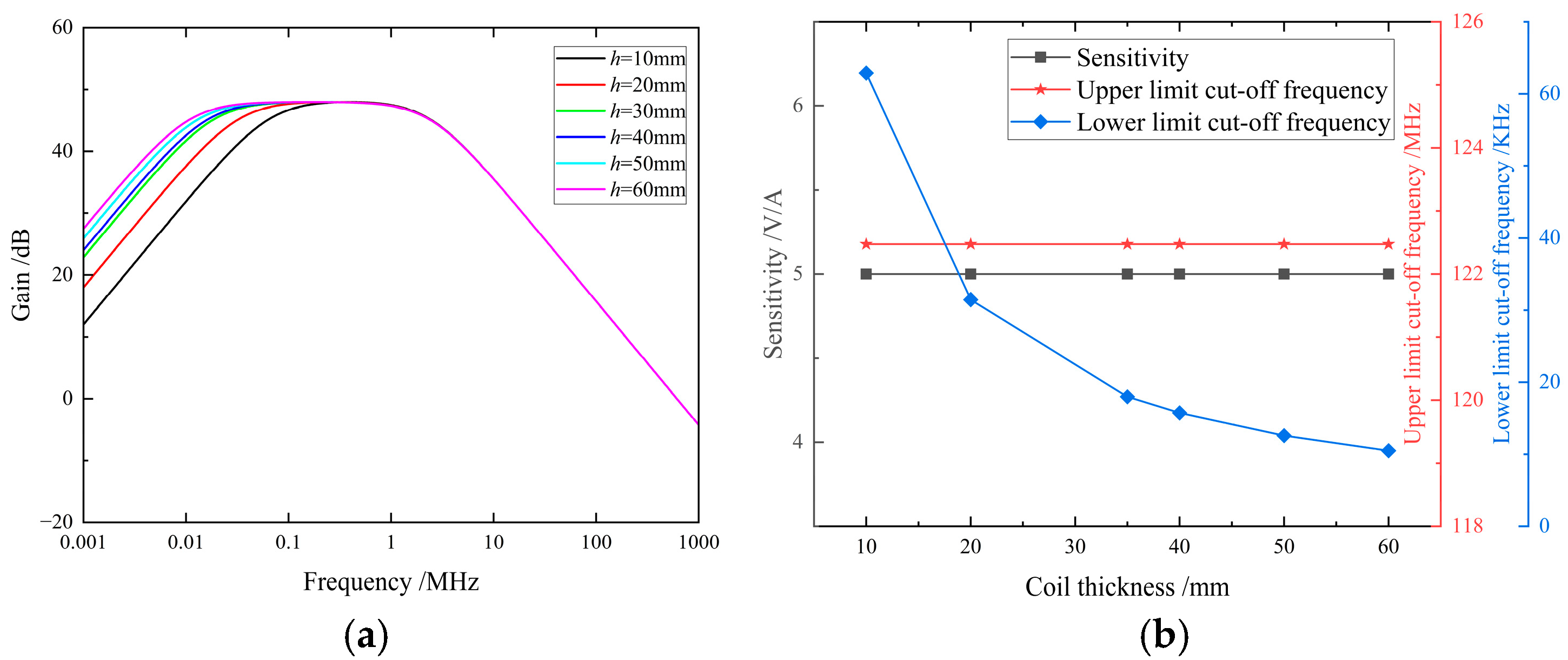
The simulation results demonstrating the impact of coil core thickness variation on sensor performance are presented in Figure 7. The curves reveal that as the coil core thickness increases from 10 mm to 60 mm, the sensor’s sensitivity and upper cutoff frequency remain unaffected, while the lower cutoff frequency decreases from 62.89 kHz to 10.5 kHz. The frequency response curves exhibit a leftward extension, showing an overall increasing trend in bandwidth.
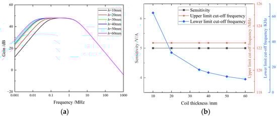
Figure 7.
(a) The influence of coil core thickness on amplitude–frequency characteristics. (b) The influence of the coil core thickness on the performance indicators.
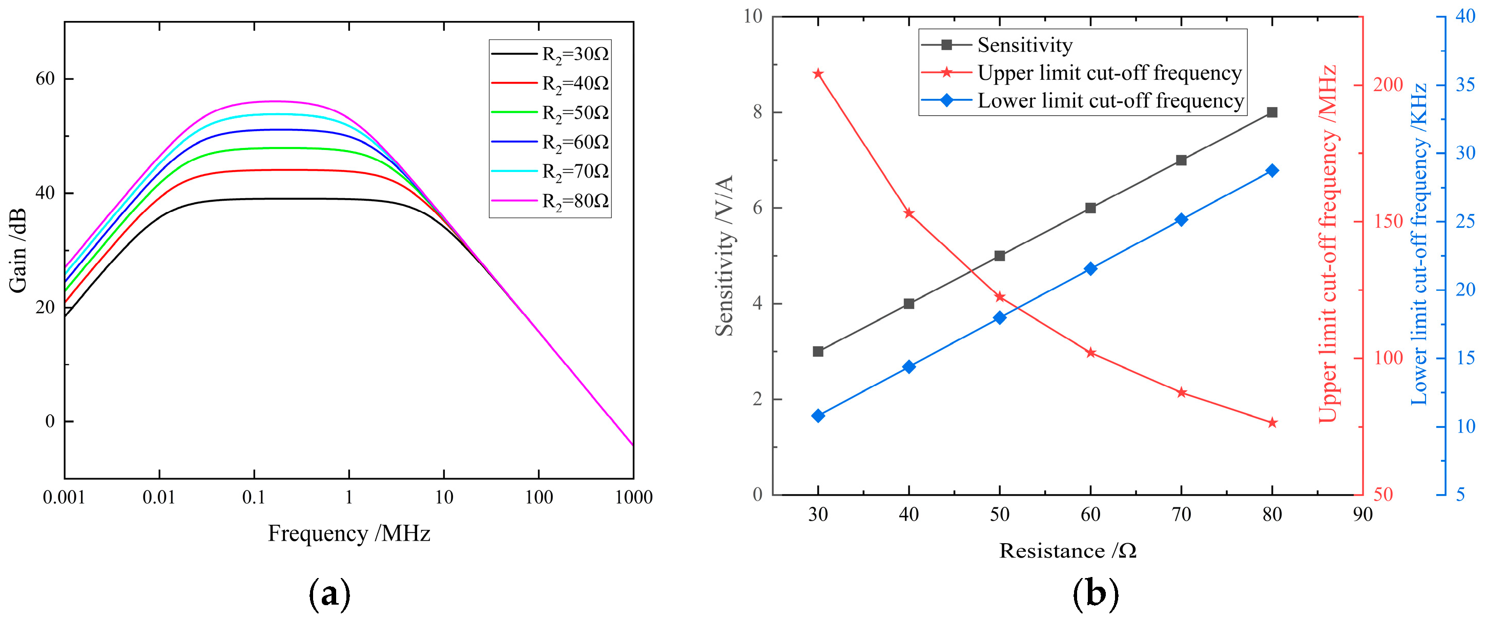
The simulation results of the sampling resistance’s influence on sensor performance are shown in Figure 8. The curves indicate that as the sampling resistance increases from 30 Ω to 80 Ω, the sensor’s sensitivity improves from 3 V/A to 8 V/A, while the upper cutoff frequency decreases from 204.12 MHz to 76.55 MHz, and the lower cutoff frequency reduces from 10.81 kHz to 28.75 kHz. The frequency response curves exhibit a leftward extension with increased peak values, showing an overall decreasing trend in bandwidth.
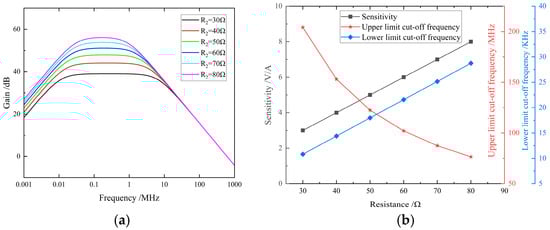
Figure 8.
(a) The influence of the sampling resistors on the amplitude–frequency characteristics. (b) The influence of the sampling resistors on the performance indicators.
4. Optimal Sensor Parameter Design
4.1. Multi-Objective Particle Swarm Optimization Algorithm
Due to the inherent trade-off between high sensitivity and wide frequency bandwidth in high-frequency current sensors, this study establishes a multi-objective particle swarm optimization (MOPSO) model to achieve optimal sensor parameter design.
The proposed model is developed based on the conventional particle swarm algorithm, with its fundamental principle inspired by the simulation of bird flock foraging behavior to search for a set of Pareto optimal solutions in multidimensional space [26]. Furthermore, the algorithm maintains an external archive to store non-dominated solutions, which is continuously updated to ensure the preservation of optimal solution sets. This archive serves to guide the particle search process, where each particle dynamically updates its position and velocity according to the following equations:
In the equations, j denotes the particle index, i represents the dimension of the optimization problem, and vi,j(t) indicates the velocity of the j-th particle at iteration t. w is the inertia weight factor characterizing the particle’s ability to maintain its previous velocity; c1 and c2 are learning factors representing individual and social learning capabilities, respectively; r1 and r2 are random numbers within [0,1] introducing stochasticity to the search process; pi,j denotes the particle’s personal best position; while pg,j represents a solution from the Pareto front, i.e., the global best solution in the external archive.
Furthermore, the algorithm employs crowding distance to calculate inter-particle distances and evaluate solution space distribution characteristics, as expressed by the following equation:
where di represents the crowding distance of particle i, and denote the objective function values of adjacent particles along the k-th objective dimension, respectively, while and indicate the maximum and minimum values of the k-th objective. During iteration, solutions with smaller crowding distances are selected from the external archive to guide the swarm, thereby promoting broader distribution across the Pareto front.
The flowchart of the MOPSO algorithm is shown in Figure 9.
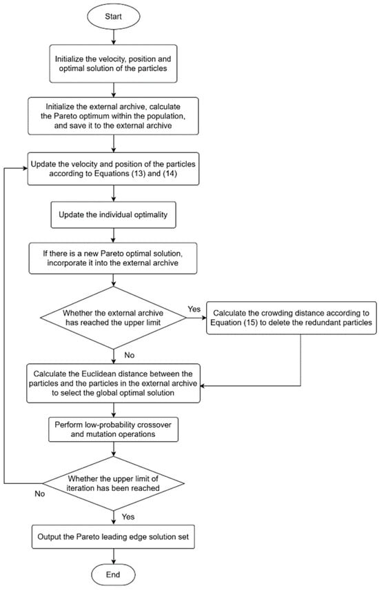
Figure 9.
Flowchart of the MOPSO algorithm.
4.2. Model Establishment
In this section, the multi-objective particle swarm optimization model is configured with cognitive factor c1 = 1.8, inertia weight w = 0.65, population size = 100, and maximum iterations = 300.
The objective functions are formulated according to the sensor design requirements as follows:
where B represents the bandwidth, and K denotes the sensitivity.
First, considering the targeted cable partial discharge signals with pulse rise times typically within 20 ns and decay times below 200 ns, the Rogowski coil must operate in a self-integrating mode (L >> R + R2) suitable for fast-pulse, high-frequency current measurement [22]. Second, structural parameters, including coil inner/outer diameters and thickness, were constrained within practical ranges based on cable dimensions to ensure sensor portability and installation feasibility. Finally, while larger sampling resistors (R2) increase sensitivity, practical implementation requires impedance matching at the UHFCT output; therefore, a 50 Ω sampling resistor was selected for model optimization to better accommodate cable partial discharge detection requirements [25].
Therefore, the constraint conditions are established as follows:
4.3. Analysis of Optimization Results
The Pareto frontier obtained by the multi-objective particle swarm algorithm consists of 30 non-dominated Pareto optimal solutions, as shown in Figure 10.
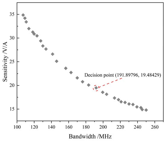
Figure 10.
Pareto frontier curve.
This study employs a defined figure of merit (FOM) to select the optimal decision point, with the FOM expressed as follows:
The FOM represents the geometric mean of bandwidth and sensitivity, reflecting the current sensor’s comprehensive capability to maintain high sensitivity across a wide frequency range, with higher values indicating superior overall performance, as demonstrated by selected typical data points in Table 2.
Table 2.
Typical points of quality factors.
Table 2 reveals that these points exhibit quality factors clustered near the maximum values. While point (110.73, 33.76) demonstrates higher sensitivity, its bandwidth is relatively narrow. Conversely, point (234.69, 15.82) offers wider bandwidth but lower sensitivity. The decision point (191.90, 19.48) achieves optimal balance between these parameters.
The marginal rate of substitution analysis indicates that left of this decision point, each 1 V/A sensitivity reduction yields 8.1 MHz bandwidth improvement, whereas right of this point, the same sensitivity sacrifice provides only 4.3 MHz bandwidth gain, confirming this location as the critical point of performance transition.
Considering both sufficient sensitivity for noise-resistant signal coupling and adequate bandwidth requirements for practical engineering applications, the hardware parameters at this decision point were selected as the design baseline for fabricating the UHF current transformer.
The final design specifications adopted Ni-Zn ferrite as the core material, with a 30 mm inner radius, 60 mm outer radius, 35 mm coil core thickness, 0.5 mm wire diameter, and 8 turns. A 50 Ω sampling resistor is recommended but adjustable, housed in a metal casing with BNC output terminals.
5. Sensor Performance Evaluation
To validate the performance of the designed sensor, this study conducted comprehensive experiments. First, frequency response tests were performed to verify the sensor’s sensitivity and bandwidth characteristics. Subsequently, a partial discharge signal detection platform was established to evaluate the sensor’s practical signal extraction capability.
5.1. Frequency Response Testing
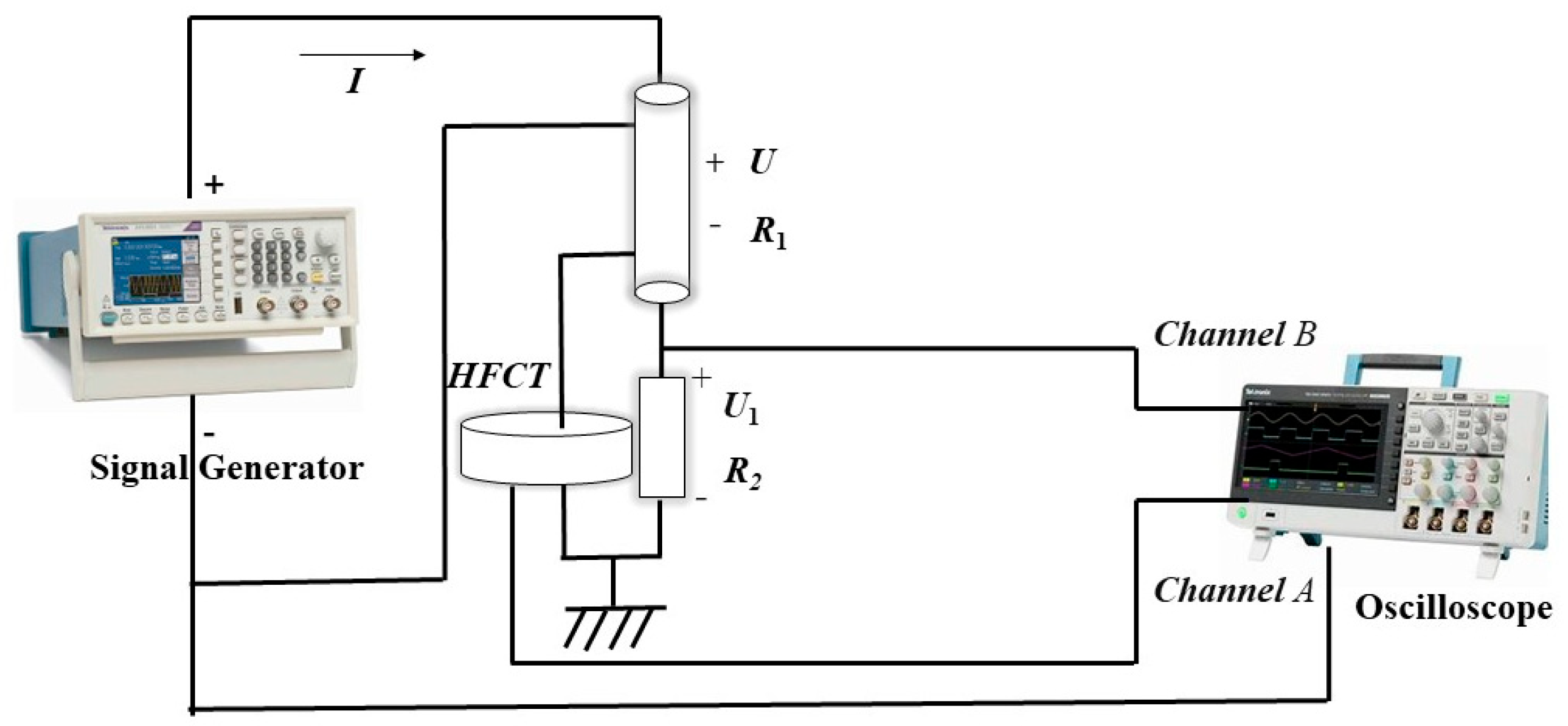
The experimental schematic is configured as follows: a signal generator forms a series circuit with the UHFCT and protective resistor R1 of Tengsong Technology in Shenzhen, China. The UHFCT connects to oscilloscope Channel A through sampling resistor R2, while Channel B monitors the voltage across R1. The constant amplitude sinusoidal frequency-sweep signal was generated by an AFG31000 signal generator of Teck Technology in Shanghai, China starting at 300 kHz with progressively increasing frequency. The input voltage U1, loop current I, and output voltage U were synchronously monitored and recorded in real time using a DPO5204B oscilloscope of Teck Technology in Shanghai, China.
The schematic diagram of the frequency response experiment is shown in Figure 11.
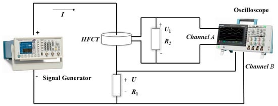
Figure 11.
Schematic diagram of frequency response experiment.
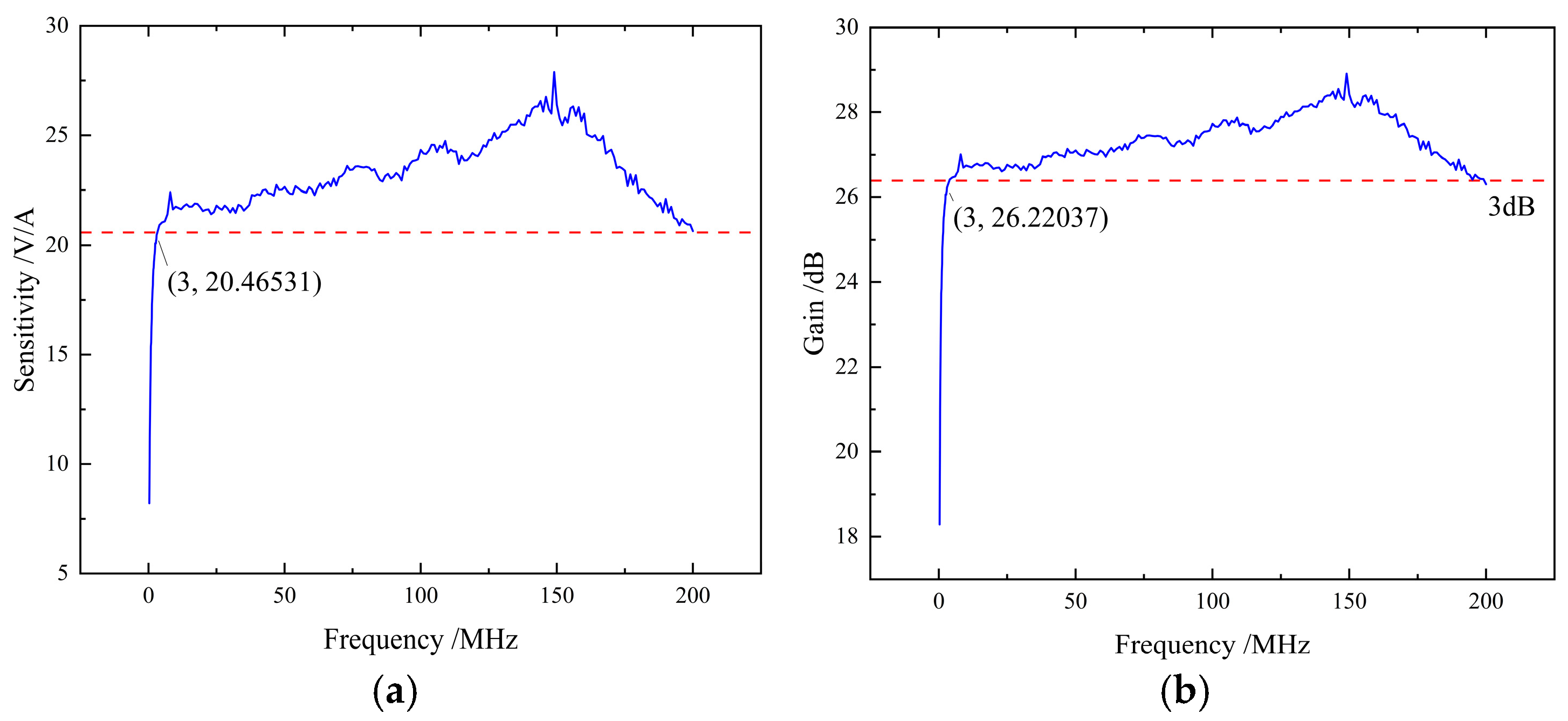
With the sampling resistor set to 50 Ω, the tested frequency response of the sensor across the 300 kHz–200 MHz range is shown in Figure 12. The frequency response curve demonstrates that the designed high-frequency current sensor maintains sensitivity no lower than 20.46 V/A within the 3 MHz–200 MHz range, exhibiting excellent signal coupling performance. Conversion of the frequency response amplitude to gain (dB) yields the gain curve, which reveals a lower −3 dB cutoff frequency of approximately 3 MHz and an upper −3 dB cutoff frequency of about 200 MHz.
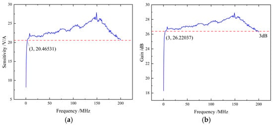
Figure 12.
(a) Sensitivity curve in frequency response. (b) Gain curve in frequency response.
5.2. Partial Discharge Signal Testing
The partial discharge signal test follows a similar schematic to the frequency response test, with resistor R1 replaced by a 40 m long RG58 coaxial communication cable. Partial discharge signals at varying frequencies were injected from the cable termination through an AFG31000 series signal generator. At the cable’s grounding wire, both the designed sensor and a conventional high-frequency current sensor for cable partial discharge detection simultaneously couple the signal. The sensor output was transmitted via the BNC interface to a DPO5204B oscilloscope to record reflected signals at the cable input terminal, thereby validating the coupling capability of the designed ultra-high-frequency through-type current sensor for cable partial discharge detection. The schematic diagram of the partial discharge test experiment is shown in Figure 13.
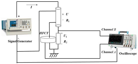
Figure 13.
Partial discharge signal test diagram.
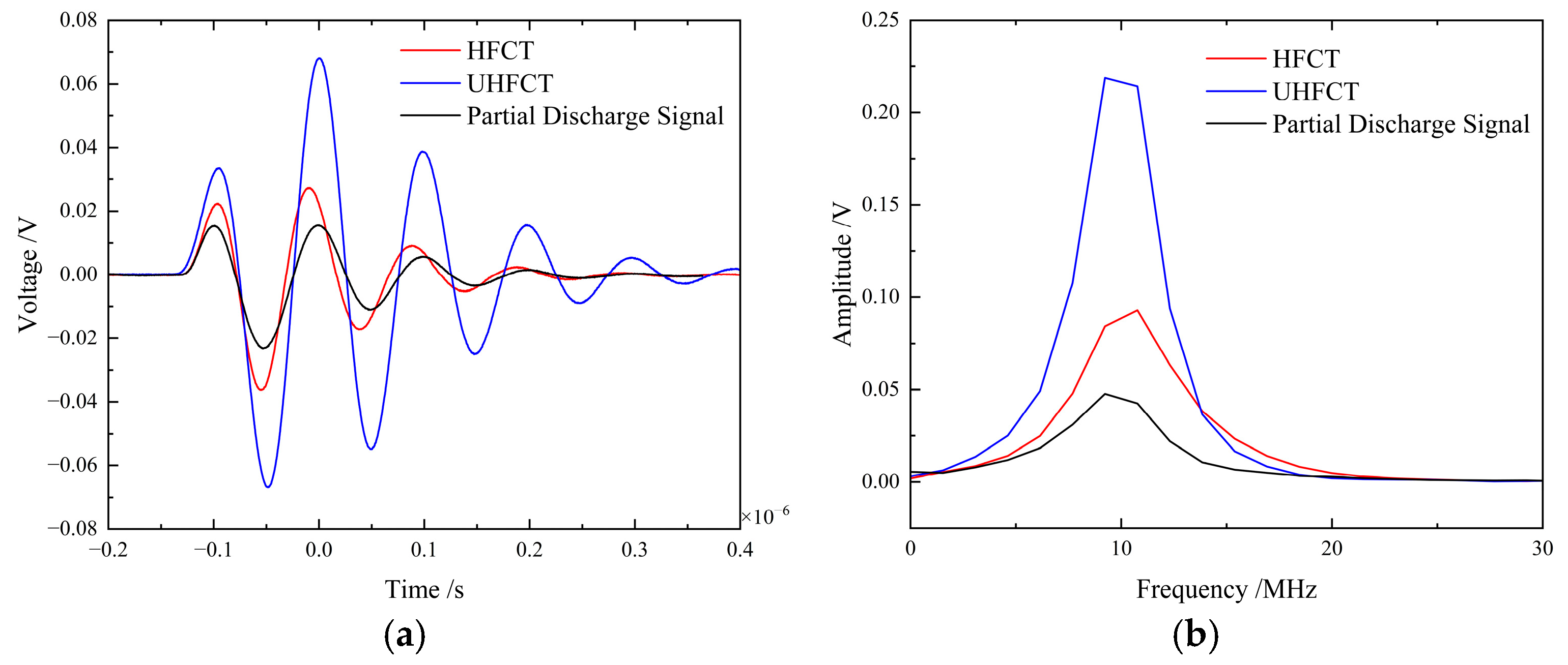
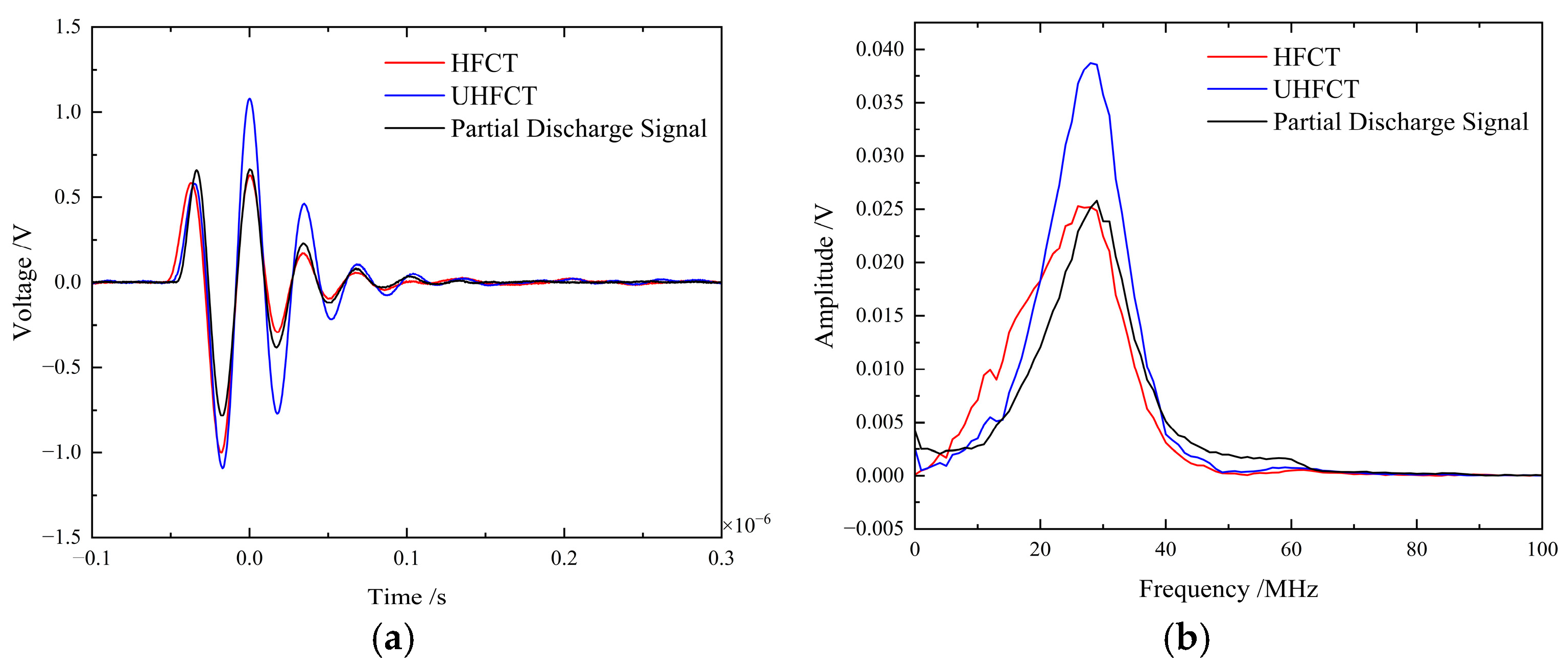
This study generates partial discharge simulation signals based on the double-exponential decay model [27], with the central frequency initially set to 10 MHz.
Figure 14 compares the coupling performance between the UHFCT (the ultra-high-frequency current transformer designed in this study) and a conventional HFCT (high-frequency current transformer). Both sensors demonstrate effective coupling capability for cable partial discharge signals. However, the UHFCT exhibits higher gain with more distinguishable waveforms that are less susceptible to noise interference.
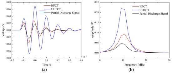
Figure 14.
(a) Time-domain comparison waveform of 10 MHz partial discharge coupled signals. (b) Frequency-domain comparison waveform of coupled signals.
Subsequent tests evaluated the coupling performance with partial discharge signals centered at 30 MHz.
Their coupling performance comparison is shown in Figure 15. The results demonstrate that the UHFCT maintains effective signal coupling capability while the HFCT reaches its cutoff frequency and exhibits phase distortion in the frequency domain.
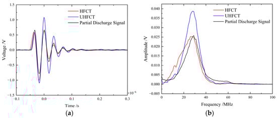
Figure 15.
(a) Time-domain comparison waveform of 30 MHz partial discharge coupled signals. (b) Frequency-domain comparison waveform of coupled signals.
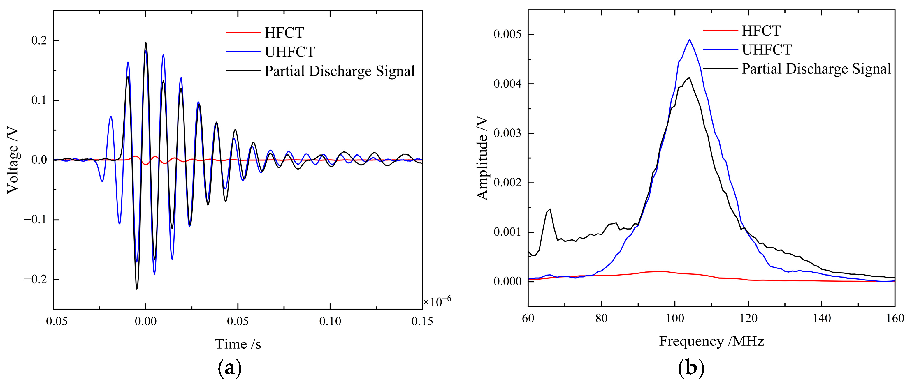
Following this phase, the central frequency of the partial discharge signal was set to 100 MHz to further evaluate the coupling performance.
The test results are illustrated in Figure 16, demonstrating that the UHFCT successfully extracted the partial discharge signal, whereas the HFCT failed to maintain effective coupling with the partial discharge signal.
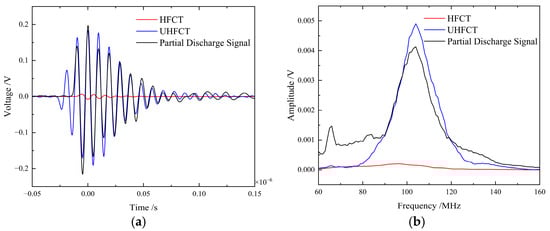
Figure 16.
(a) Time-domain comparison waveform of 100 MHz partial discharge coupled signals; (b) Frequency-domain comparison waveform of coupled signals.
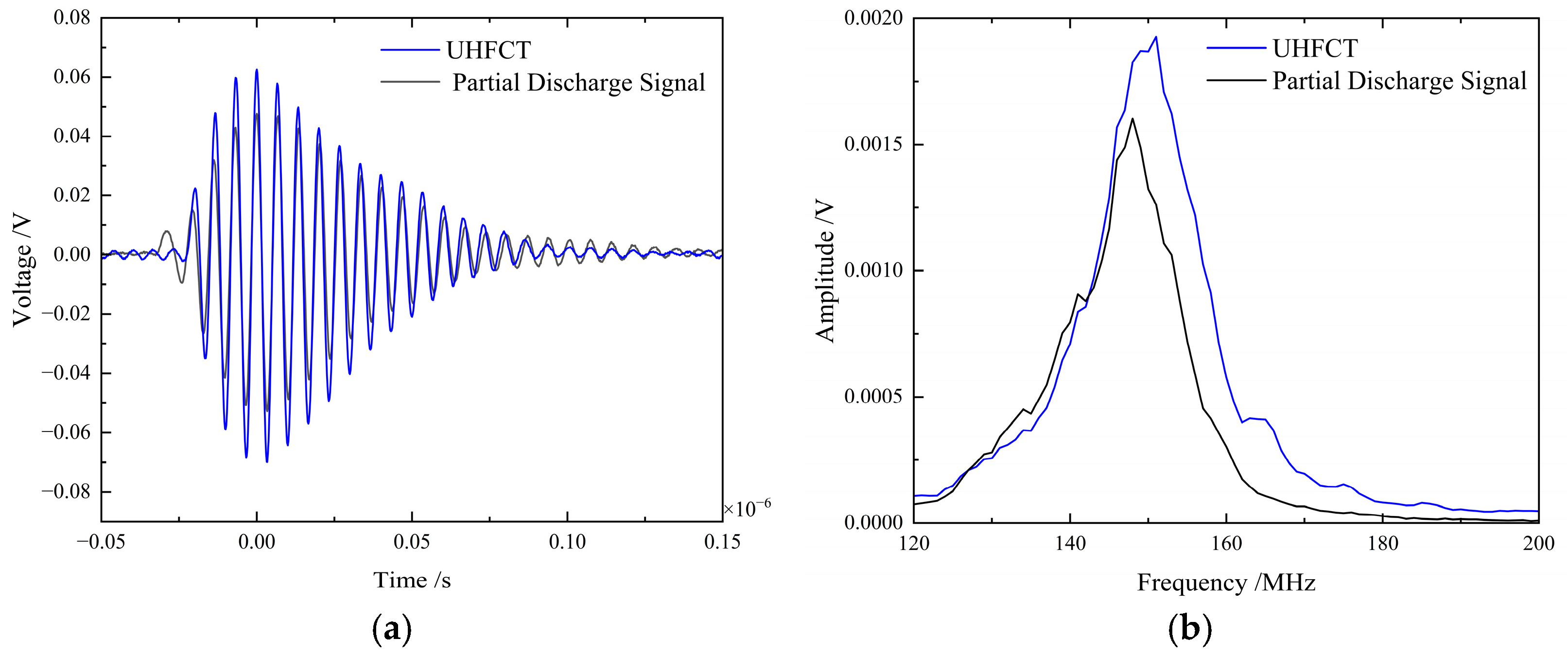
To further validate the bandwidth and frequency response flatness, this study conducted partial discharge signal testing with a center frequency of 150 MHz.
Figure 17 presents both time-domain and frequency-domain analyses demonstrating the UHFCT’s effective extraction capability for partial discharge signals at 150 MHz. In contrast, HFCT is no longer capable of coupling signals.
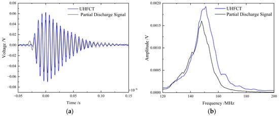
Figure 17.
(a) Time-domain comparison waveform of 150 MHz partial discharge coupled signals. (b) Frequency-domain comparison waveform of coupled signals.
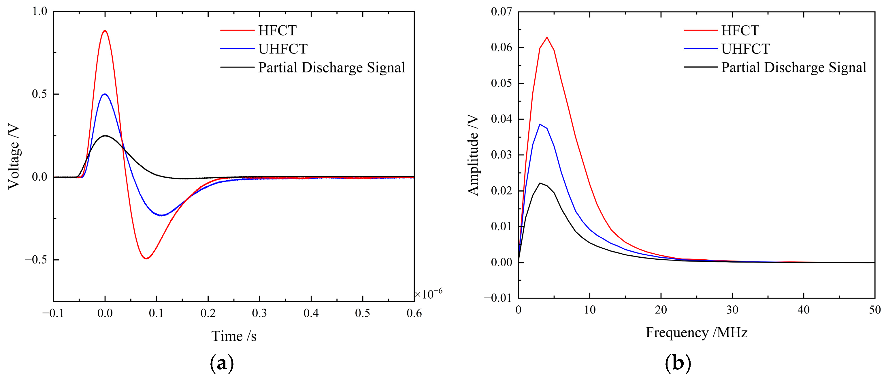
Finally, to validate the sensor’s response capability at boundary frequencies, experimental tests were conducted at both 3 MHz and 200 MHz, respectively.
The test results under a partial discharge signal with a center frequency of 3 MHz are presented in Figure 18. At the frequency of 3 MHz, both sensors demonstrated effective coupling capability for cable partial discharge signals. Although the UHFCT exhibited lower gain, it maintained superior frequency stability without spectral shift, achieving higher measurement accuracy than the HFCT.
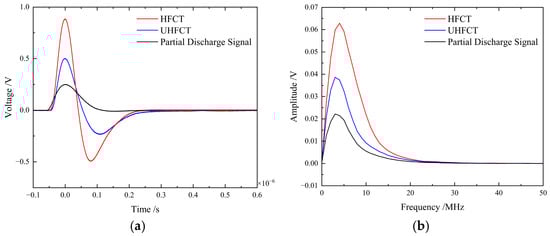
Figure 18.
(a) Time-domain comparison waveform of 3 MHz partial discharge coupled signals. (b) Frequency-domain comparison waveform of coupled signals.
Figure 19 demonstrates the UHFCT’s coupling capability in both time and frequency domains, confirming its effective extraction of partial discharge signals at this ultra-high-frequency range. The conventional HFCT was excluded from comparison due to its inherent inability to couple signals in this frequency band.
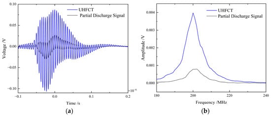
Figure 19.
(a) Time-domain comparison waveform of 200 MHz partial discharge coupled signals. (b) Frequency-domain comparison waveform of coupled signals.
The experimental results verify that the designed sensor demonstrates effective coupling capability for cable partial discharge signals across all tested frequency bands.
6. Conclusions
This paper presents an optimized design method for an ultra-high-frequency through-core current sensor for cable partial discharge detection, yielding the following conclusions:
- (1)
- The number of turns exhibits a negative correlation with sensitivity, showing a decreasing trend as turns increase. In contrast, the sampling resistor demonstrates a positive correlation with sensitivity. Other hardware parameters do not affect sensor sensitivity.
- (2)
- The coil outer radius and sampling resistor are negatively correlated with bandwidth, which decreases as they increase. Conversely, coil thickness, number of turns, and inner radius show positive correlations with bandwidth. Wire diameter does not influence sensor bandwidth.
- (3)
- The designed UHF through-core current sensor features a simple structure, with frequency response tests confirming its compatibility with both high bandwidth and sensitivity. Partial discharge signal tests verify its effective coupling capability for cable PD signals across low, medium, and high-frequency ranges.
Future research directions include integrating the sensor with AI-based PD diagnostics for automated fault prediction, optimizing its miniaturization for dense cable systems through field validation under diverse environmental conditions, and extending its frequency response to GHz ranges to enhance advanced PD detection capabilities.
Author Contributions
Conceptualization, H.L. (Hongda Li) and H.L. (Hongjing Liu); methodology, N.H. and J.T.; software, W.M.; validation, C.G., N.H., and J.T.; formal analysis, B.C.; investigation, W.M. and B.C.; data curation, H.L. (Hongda Li) and R.B.; writing—original draft preparation, H.L. (Hongjing Liu) and N.H.; writing—review and editing, J.T.; visualization, X.L.; supervision, B.C. All authors have read and agreed to the published version of the manuscript.
Funding
This research was funded by the Science and Technology Project of State Grid Corporation of China (B7022324000T).
Data Availability Statement
The original contributions presented in the study are included in the article; further inquiries can be directed to the corresponding author.
Conflicts of Interest
The authors declare that this study was funded by and from Beijing Electric Power Research Institute. The funders were not involved in the design of the research, the collection, analysis, interpretation of the data, nor in the writing of this article or the decision on whether to publish it.
References
- Wei, B. Study on Partial Discharge On-Line Monitoring and Fault Characteristics of 110 kV High Voltage XLPE Cable Accessories. Master’s Thesis, North China Electric Power University, Beijing, China, 2004. [Google Scholar]
- Ma, G.M.; Li, C.R.; Chen, X.W.; Jiang, J.; Ge, Z.D.; Chang, W.Z. Numerical sensor design for partial discharge detection on power cable joint. IEEE Trans. Dielectr. Electr. Insul. 2015, 22, 2311–2319. [Google Scholar] [CrossRef]
- Zhou, X.H.; Zeng, P.; Liu, Z.G.; Chen, Y.; Cheng, A.; Zhang, Z.Q.; Cai, X.J. Analysis of electromagnetic wave propagation characteristics of partial discharge in cable intermediate joint and optimization design of sensor. Hunan Electr. Power 2024, 44, 81–86. [Google Scholar]
- Hung, Y.C.; Tang, K.W.; Li, S.S. Mode Localized Piezoelectric Resonator Design and Implementation for Electrical Current Sensing. In Proceedings of the 2024 IEEE SENSORS, Kobe, Japan, 20–23 October 2024; pp. 1–4. [Google Scholar]
- Liu, S.; Chen, P.; Luo, J.; Chen, Y.; Liu, B.; Xiao, H.; Yan, W.; Ding, W.; Bai, Z.; He, J.; et al. Nano-Optomechanical Resonators Based Graphene/Au Membrane for Current Sensing. J. Light. Technol. 2022, 40, 7200–7207. [Google Scholar] [CrossRef]
- Tao, P. Local Leakage Location Method for High-Voltage Insulating Equipment Based on Optical Fiber Sensors. Electr. Drive 2023, 53, 91–96. [Google Scholar]
- Zhuang, H.; Qi, Y.J.; Li, B.; Liu, Y.W. Design of Partial Discharge Detection System Based on sic-based Photoelectric Sensor. Semicond. Optoelectron. 2018, 39, 712–715+721. [Google Scholar]
- State Grid Corporation of China. Technical Specification for Live Detection Instruments of Power Equipment—Part 5: Technical Specification for High-Frequency Partial Discharge Live Detector: Q/GDW 11304.5—2015; China Electric Power Press: Beijing, China, 2015. [Google Scholar]
- Tang, Z.G.; Jiang, T.T.; Yu, Z.Q. Research on high frequency current method for detecting partial discharge of capacitors. Electr. Mach. Control 2019, 23, 18–25+33. [Google Scholar]
- Tang, Z.G.; Jiang, T.T.; Zhang, L.G. Study on sensitivity of high frequency current method for detecting capacitor partial discharge. High Volt. Appar. 2018, 54, 9–15. [Google Scholar]
- Li, H.N. Partial Discharge Detection Method of High Voltage Cable Joint. Master’s Thesis, North China Electric Power University, Beijing, China, 2011. [Google Scholar]
- Jiang, J.B.; Chen, G.F.; Luo, Z.; Fang, C.H.; Zou, Y.A.; Zhao, L. Research and design of Roche coil for partial discharge signal measurement. High Volt. Appar. 2025, 61, 63–71. [Google Scholar]
- Fu, S.; Deng, E.; Peng, C.; Zhang, G.; Zhao, Z.; Cui, X. Method of turns arrangement of noncircular Rogowski coil with rectangular section. IEEE Trans. Instrum. Meas. 2020, 70, 9000310. [Google Scholar] [CrossRef]
- Huang, Y.G. Experimental study on non-ideal working condition of Roche coil. Electron. Meas. Technol. 2018, 41, 38–41. [Google Scholar]
- Gong, J.; Yang, D.; Zhou, L.X. Improvement of partial discharge pulse current sensor in transformer. J. Electr. Power Sci. Technol. 2007, 4, 68–71. [Google Scholar]
- Giussani, R.; Zachariades, C.; Foxall, M.; Renforth, L.; Seltzer-Grant, M. A novel electrical sensor for combined online measurement of partial discharge (OLPD) and power quality (PQ). In Proceedings of the International Symposium on High Voltage Engineering, Pilsen, Czech Republic, 23–28 August 2015. [Google Scholar]
- Xu, Y.; Gu, X.; Liu, B.; Hui, B.; Ren, Z.; Meng, S. Special requirements of high frequency current transformers in the on-line detection of partial discharges in power cables. IEEE Electr. Insul. Mag. 2016, 32, 8–19. [Google Scholar] [CrossRef]
- Zhu, J.; Zhang, Q.; Jia, J.; Tao, F.; Yang, L.; Yang, L. Design of a Rogowski coil with a magnetic core used for measurements of nanosecond current pulses. Plasma Sci. Technol. 2006, 8, 457–460. [Google Scholar]
- Gong, H. Modeling Method, and Development Technology of High Frequency Current Sensor Based on Electromagnetic Induction Principle. Ph.D. Thesis, Huazhong University of Science and Technology, Wuhan, China, 2020. [Google Scholar]
- Cooper, J. On the high-frequency response of a Rogowski coil. J. Nucl. Energy Part C Plasma Phys. Accel. Thermonucl. Res. 2002, 5, 285. [Google Scholar] [CrossRef]
- Naito, K.; Mizuno, Y. A study on probabilistic assessment of contamination flashover of high voltage insulator. IEEE Trans. Power Deliv. 1995, 10, 1378–1384. [Google Scholar] [CrossRef]
- Fang, Z.; Zhao, Z.Y.; Qiu, Y.C.; Li, S. Analysis of high frequency characteristics of Rogowski coil. High Volt. Eng. 2002, 8, 17–18+21. [Google Scholar]
- Wang, L. Development of High Frequency Current Sensor Based on Ni-Zn Ferrite Soft Magnetic Material. Master’s Thesis, North China Electric Power University, Beijing, China, 2018. [Google Scholar]
- Liu, Y.P.; He, S.J.; Bao, D.X.; Ren, X.Y. Development trend of soft magnetic materials. J. Magn. Mater. Devices 2003, 34, 26–29. [Google Scholar]
- Deng, J.Y.; Wang, X.H.; Nie, Y.X. Design of high frequency current sensor for on-line monitoring of cable joints. Power Electron. Technol. 2023, 57, 33–36. [Google Scholar]
- Zhang, S.F.; Jia, D.L.; Gong, B. Structure optimization of layered injection streamlined spool based on multi-objective particle swarm optimization. Oil Field Mach. 2025, 54, 46–56. [Google Scholar]
- Wang, D.F.; Kong, H.Y.; Wu, L.; Li, W.J. Simulation research on signal propagation characteristics of XLPE cable local discharge. Hubei Electr. Power 2016, 40, 53–57+62. [Google Scholar]


Disclaimer/Publisher’s Note: The statements, opinions and data contained in all publications are solely those of the individual author(s) and contributor(s) and not of MDPI and/or the editor(s). MDPI and/or the editor(s) disclaim responsibility for any injury to people or property resulting from any ideas, methods, instructions or products referred to in the content. |
© 2025 by the authors. Licensee MDPI, Basel, Switzerland. This article is an open access article distributed under the terms and conditions of the Creative Commons Attribution (CC BY) license (https://creativecommons.org/licenses/by/4.0/).