Inverse Design of Microstrip Antennas Based on Deep Learning

Abstract

This paper introduces a novel inverse design framework that combines pixelated microstrip antenna modeling, convolutional neural network (CNN), and binary particle swarm optimization (BPSO) to automate the process of generating antenna structures from specified performance targets. The framework operates through a streamlined workflow: the radiating patch is discretized into a 10 × 10 binary matrix to enable combinatorial design space exploration; a CNN is trained on 150,000 simulated datasets to predict S-parameters as a surrogate for time-consuming electromagnetic simulations; and BPSO optimizes pixel states guided by a fitness function that minimizes reflection coefficients at target frequencies. By representing the patch as binary pixels, the approach exponentially expands the design space from traditional parametric limits to about 10³⁰ combinatorial possibilities, overcoming the inefficiencies of manual trial-and-error design. Comparative studies with genetic algorithms (GAs) and simulated annealing (SA) demonstrate that the BPSO-CNN framework achieves faster convergence and lower S11 error at target frequencies. This work not only advances the state of the art in intelligent antenna design but also provides a scalable paradigm for automated electromagnetic device optimization.

1. Introduction

Microstrip antennas have gained widespread attention in wireless communication systems due to their light weight, low profile, and planar structure, which are ideal for integration with modern portable devices [1,2,3,4,5]. In the realm of 5G and future 6G communication technologies, microstrip antennas play a crucial role in enabling high-speed data transmission while maintaining compact structure, making them indispensable components for smartphones, tablets, and wearable devices. Traditional methods to design a microstrip antenna often rely on full-wave simulation software. Engineers modify parameters such as patch size, substrate thickness, and feed location to observe the impacts of the structure parameters on antenna performance and find the optimal parameters [6,7]. This conventional design approach is heavily reliant on manual parameter adjustment and repetitive full-wave simulations, leading to high computational costs and limited design flexibility, especially for complex multiband or multi-objective requirements.

Machine learning (ML) has emerged as a transformative tool in electromagnetic design, enabling data-driven prediction and optimization. Early works on ML-based antenna design focused on using artificial neural networks (ANNs) and support vector machines (SVMs) to predict performance metrics from geometric parameters [8,9]. While these models reduced simulation time, they were limited by the predefined parameter spaces, often requiring engineers to specify critical structural features (e.g., slot shapes) upfront. Recent advancements in deep learning have enabled more flexible approaches; for example, generative adversarial networks (GANs) have been used to generate antenna structures from performance targets, but their training requires sophisticated architectures and large computational resources [10,11].

Pixelated modeling represents a breakthrough in expanding design freedom. By treating each patch element as a binary pixel, the design space becomes combinatorial, allowing for arbitrary shapes that traditional parametric models cannot represent. This approach has been successfully applied in other electromagnetic design domains, such as microwave filter design, where pixelated representations enabled the creation of filters with unique frequency response characteristics. In [12], the patch resonator of the filtering power amplifier is pixelated into a 10 × 20 binary matrix. Under the optimization process of BPSO, the proposed filtering power amplifier yielded dual-band and wideband operations. Combined with CNN for feature extraction and algorithm for global optimization, pixelated modeling offers a promising solution for inverse design, where the goal is to find structures that satisfy given performance criteria, rather than optimizing predefined parameters [13,14,15,16]. In [15], the authors combined the CNN and GA to inversely design the output matching network for the power amplifier, which reduces labor-intensive optimization and human expertise. In [16], a tandem neural that consists of a CNN and inverse network was proposed to design multiband antenna without the requirement of extensive domain knowledge.

In this study, we address the limitations of traditional methods by introducing a pixelated representation of microstrip antennas, which converts geometric structures into binary matrices suitable for ML processing. Combined with a CNN for fast performance prediction and BPSO for global optimization, our framework achieves efficient inverse design, where target performance specifications directly guide the search for optimal antenna structures. A dual-band microstrip antenna operating at 2.8 and 3.7 GHz is selected as the design task of the proposed approach. The validation results demonstrate that the proposed inverse design method can generate the microstrip antenna at the desired frequencies. The proposed deep learning-based approach provides a more efficient and flexible method than the conventional design method, which has potential applications in automating design of the passive microwave components.

2. Design and Training of Deep-CNN Forward Network

2.1. Pixelated Antenna Representation

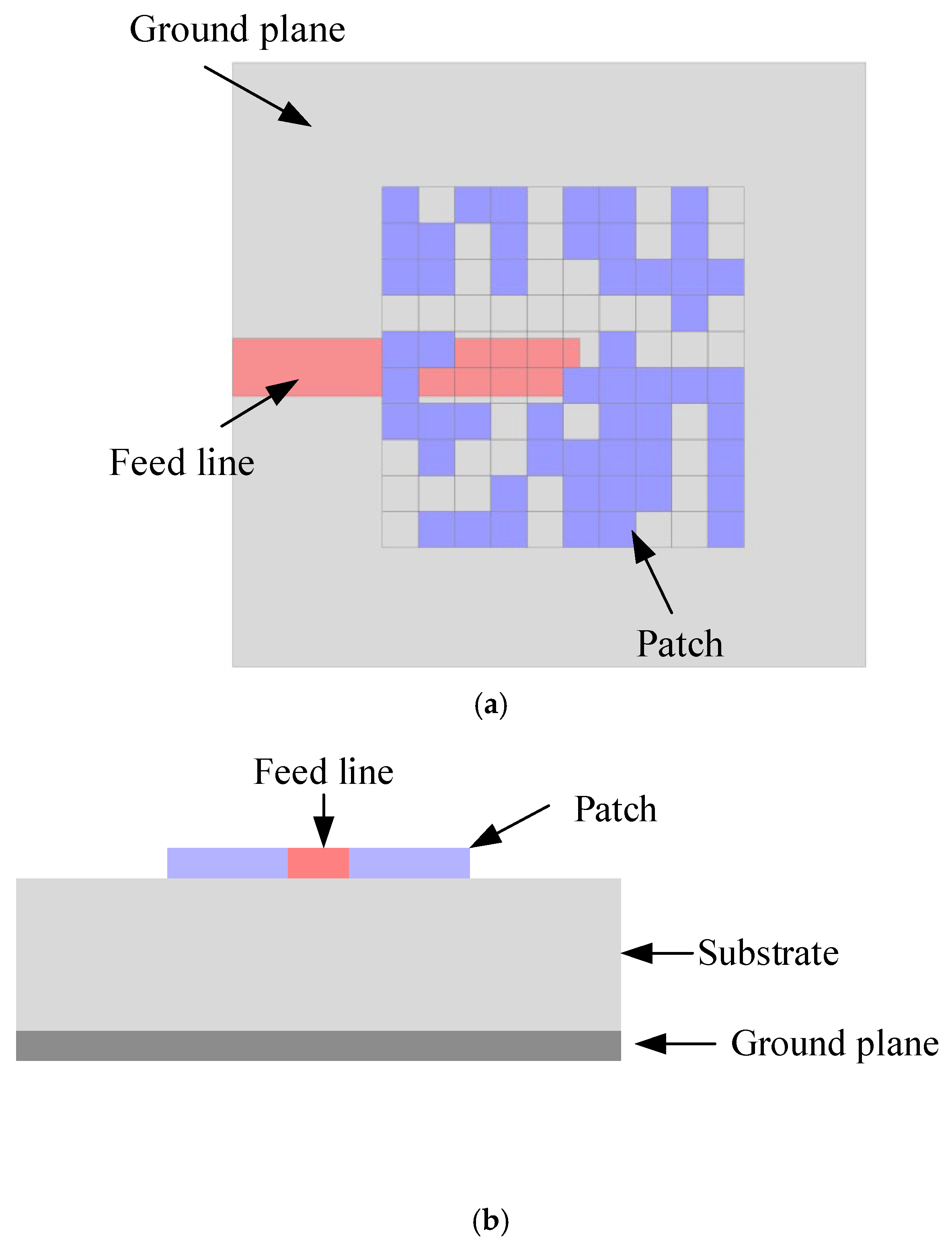
The antenna is designed in a printed circuit board substrate with a dielectric constant of 2.2 and thickness of 2.5 mm. In this study, we assumed that the dielectric substrate is an ideal lossless substrate for simplifying the initial design framework. This idealization allows us to focus on the fundamental relationships between antenna geometry and radiation characteristics without the complexity introduced by dielectric losses. This choice of 2.5 mm thickness is primarily to improve antenna bandwidth, as thinner dielectric boards tend to narrow the bandwidth, making it difficult to synthesize broadband antennas during reverse design. The increased thickness relaxes electromagnetic field constraints, facilitating wider operational bandwidth optimization. The radiating patch and the feed line are printed on the top layer (the same plane). The bottom layer is filled with copper as the ground plane of the patch antenna. The patch is divided into a 10 × 10 grid, where each pixel x_i,j ∈ {0,1} indicates the presence (“1”) or absence (“0”) of a metallic patch element, as shown in Figure 1. The total design space includes 2¹⁰⁰ configurations, which is computationally intractable for exhaustive search. The pixel size is set to 6.5 × 6.5 mm, with a 0.5 mm overlap between adjacent pixels to ensure continuous current distribution, addressing potential discontinuity issues in electromagnetic simulations [17]. The microstrip feed line is fixed in the design, as shown in the red color in Figure 1. The end of the feed line is extended to the center of the radiating patch to guarantee valid impedance matching and energy transmission.

2.2. CNN-Based Forward Prediction Model

2.2.1. Dataset Generation

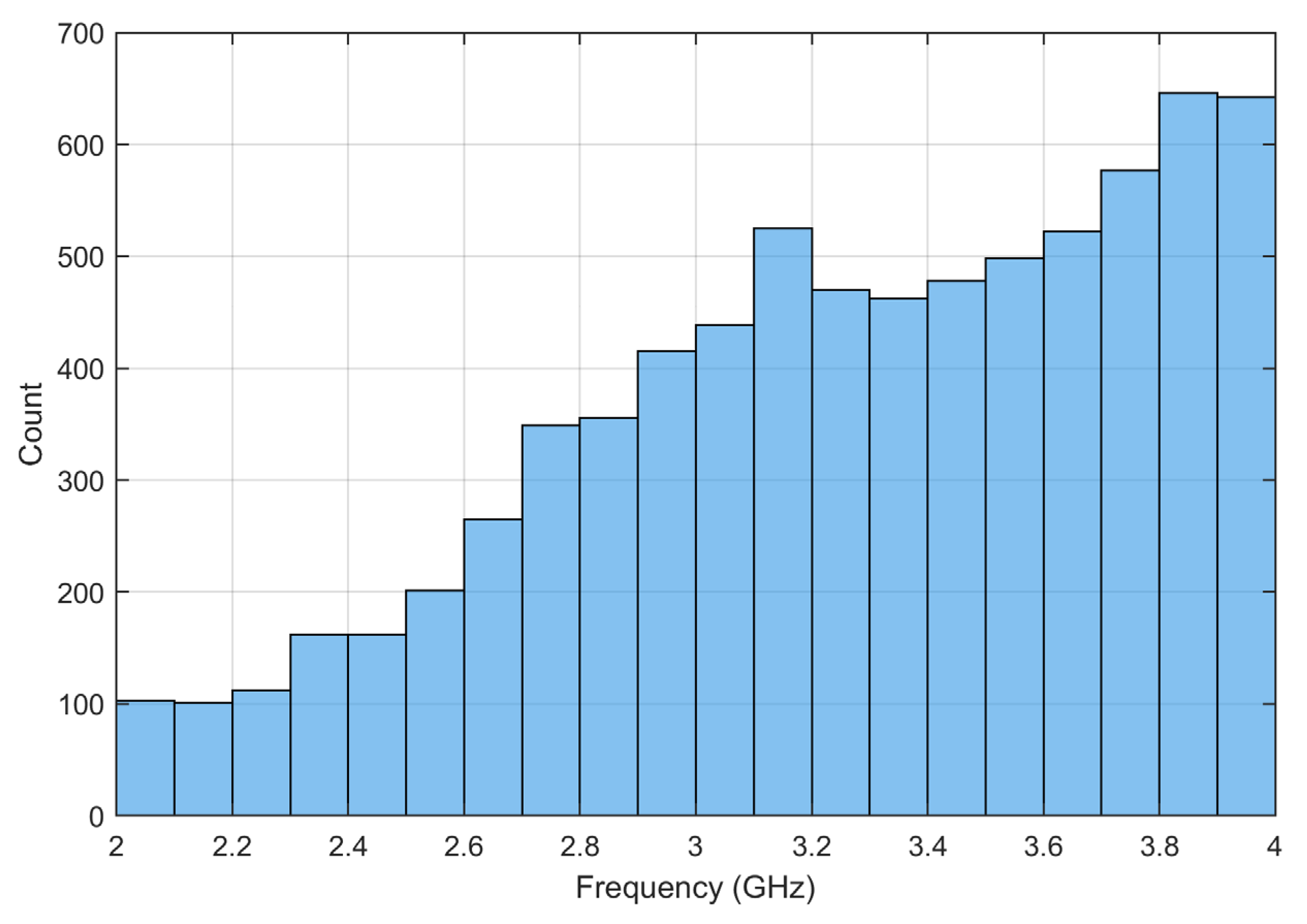
The dataset is automatedly generated by leveraging MATLAB R2022a scripts to control the full-wave electromagnetic simulation software, CST Studio Suite 2021. The sweeping frequencies in the simulation are from 2 to 4 GHz, which includes 50 points with a 0.04 GHz interval. In each data sample, the input is a random 10 × 10 matrix, while the output is the reflection coefficient (S₁₁) of the antenna. The dataset includes 150,000 samples, with 80% for training, 10% for validation, and 10% for testing. A sample is labeled “resonant” if it has at least two consecutive frequency points with S₁₁ < −10 dB, yielding 19,000 resonant samples (12.6% of total). For samples labeled as “resonant”, we determine the single “resonant frequency” as the average of all frequency points within the continuous resonant band where S₁₁ < −10 dB. This approach ensures robustness by mitigating noise and providing a representative central value for the resonant behavior. The resonant frequency distribution is depicted in Figure 2, which shows a gradual increase with frequency, indicating balanced coverage across the target band.

2.2.2. Network Architecture

We adopt the deep-CNN architecture as the forward surrogate model for the full-wave simulation software. The deep-CNN architecture is able to capture complex hierarchical features in microstrip antenna designs. In contrast to simpler CNNs, deeper networks can extract multi-level electromagnetic patterns and spatial relationships within the pixelated antenna models, which are crucial for accurately predicting S-parameters from antenna geometries. The input of the CNN is the 10 × 10 matrix that is similar to a single channel image. The output of the CNN is a one-dimensional vector with 50 elements, corresponding to the reflection coefficient of the patch antenna. The task of this deep-CNN is to accurately predict the reflection coefficient of the patch after training. The detail of the proposed deep-CNN is shown in Figure 3.

• Convolutional Layers: Ten layers with kernel sizes decreasing from 5 × 5 to 2 × 2 (5 × 5 → 5 × 5 → 4 × 4 → 4 × 4 → 3 × 3 → 3 × 3 → 3 × 3 → 2 × 2 → 2 × 2 → 2 × 2), and channel numbers varying from 32 to 128, incorporating batch normalization and ReLU activation to improve convergence.
• Fully Connected Layers: Four layers (500 → 200 → 50 → 50 neurons), with the final layer outputting S-parameter values for 50 frequency points.

2.2.3. Training and Validation

In the training process, we adopt mean squared error (MSE) as the loss function:

$$L={\displaystyle \frac{1}{P}}\sum _{i=1}^P{\left(S_i-S_i^{\prime }\right)}^2$$

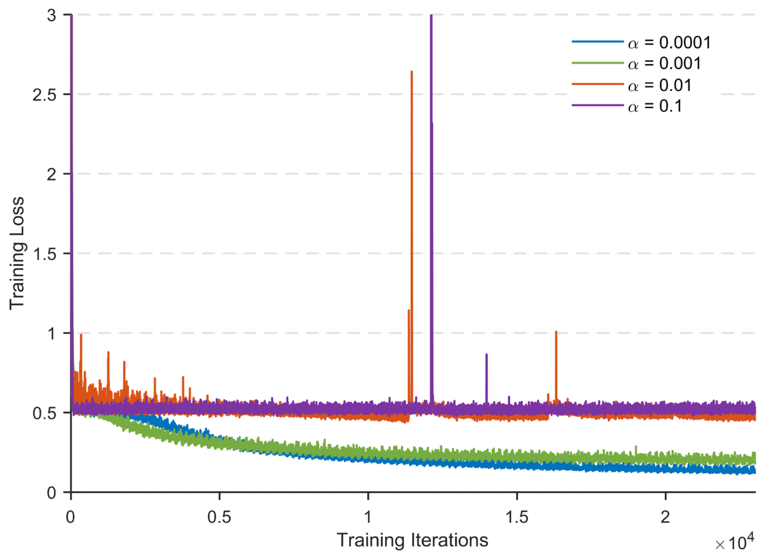
where P is the batch size, and S_i and S_i^’ are the simulated value from CST software and predicted value using CNN, respectively. The model is trained with the Adam optimizer in combination with an early stopping strategy to effectively balance the training speed and convergence stability. In order to ensure good performance of the gradient descent method, we need to set the learning rate within an appropriate range. If the learning rate is too small, it will significantly reduce the convergence speed and increase training time; if the learning rate is too large, it may cause the parameters to oscillate back and forth around the optimal solution. Therefore, the learning rate is crucial to the algorithm’s performance. Hence, we compared the impact of the learning rate on the model, as shown in Figure 4.

When the learning rate is too high, as shown in the case of α = 0.1 and α = 0.01, the loss function oscillates violently near the optimal solution, resulting in complete non-convergence. This phenomenon is often accompanied by gradient explosion issues, which can be mitigated through gradient clipping. When the learning rate is reduced to 0.001, the loss function can achieve good convergence, ultimately reaching the optimal solution through sufficient iterations. If the learning rate is too small, in the case of α = 0.0001, the convergence speed is the slowest, and the loss function eventually reaches the minimum value through sufficient iterations. However, by observing the loss function value, which rises again after decreasing, it is found that overfitting occurs under this learning rate.

In order to achieve quick convergence of the loss function in the early stages and to fine-tune the parameters in the later stages, learning rate decay is used to dynamically adjust the learning rate during training. We adopt piecewise decay of the learning rate, which is divided into three segments: the first 100 epochs use a learning rate of 0.01, the subsequent 5000 epochs adopt a learning rate of 0.001, and finally a learning rate of 0.0005 is applied.

The batch size of the data is very crucial in the training. As illustrated in Figure 5, we compared the impact of different batch sizes on model performance. When the batch size is too small, such as 128 or 256, the network receives insufficient samples per iteration. This leads to unrepresentative statistical features and increased noise, making it difficult for the model to converge. Conversely, an excessively large batch size, like 1024, causes the gradient direction to become overly stable. This can trap the model in local optima and degrade accuracy. The figure clearly shows that batch size significantly influences the convergence speed of this model. Given a final learning rate of 0.0005, a larger batch size is necessary to balance training stability and efficiency according to the noise balance theory [17]. Therefore, we selected a batch size of 512 as the optimal configuration.

The process of training a convolutional neural network surrogate model is the process of minimizing the loss function. The optimizer used during model training is Adam, with the learning rate set to piecewise decay. The model achieves convergence after training for 50,000 epochs. The training loss gradually decreases from an initial value of 6 to 0.62, while the validation loss stabilizes at 0.71, indicating that the model has strong fitting capability for the target features without significant overfitting.

The model achieves a root mean square error (RMSE) of 0.35, mean absolute error (MAE) of 0.28, and coefficient of determination (R²) of 0.94. These key regression metrics demonstrate that the model can effectively capture nonlinear relationships in the data. Once the neural network surrogate model’s training is completed, this network can be utilized to predict the S₁₁ of antenna by inputting antenna physical parameters.

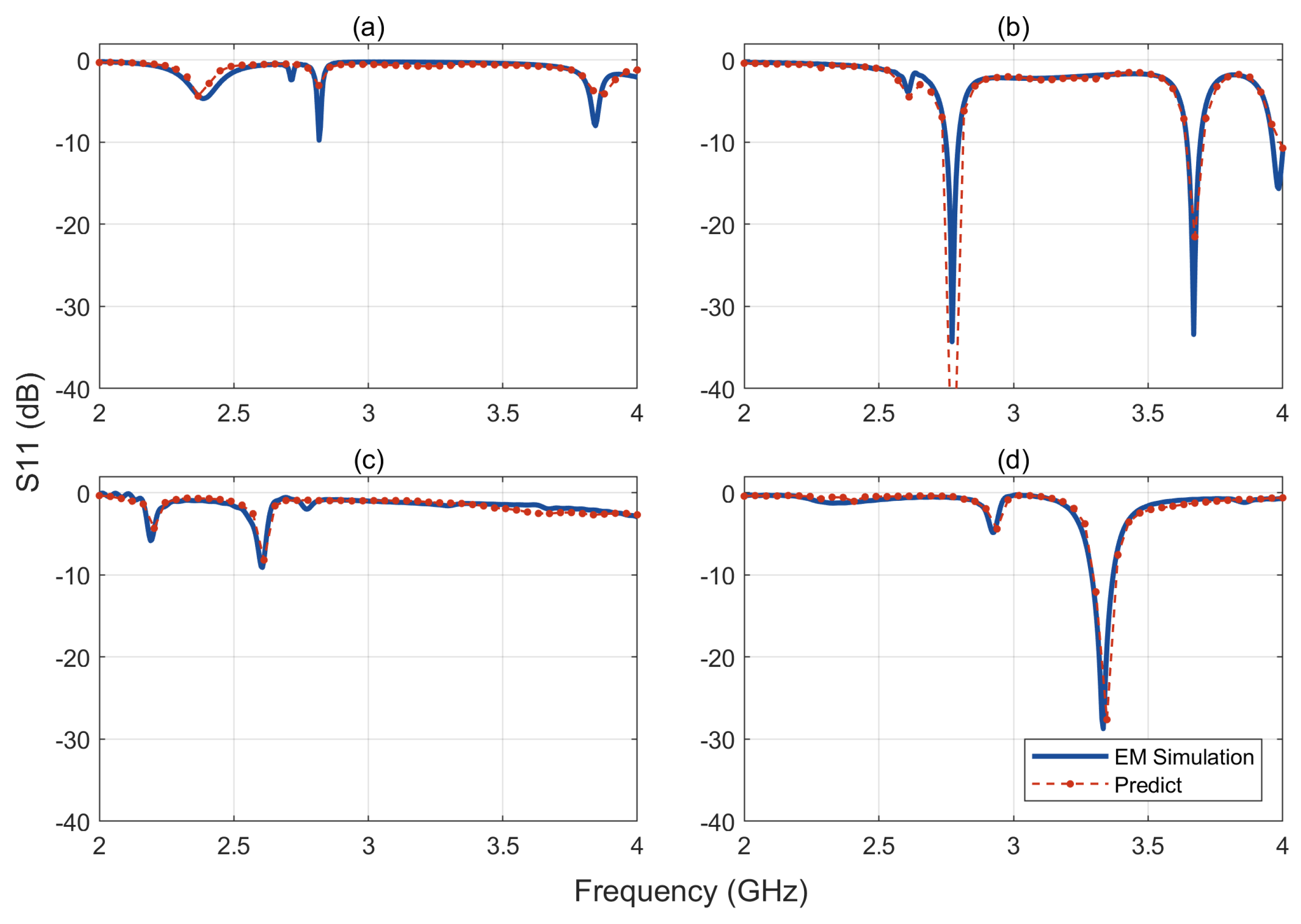
Figure 6 presents a comparison of S₁₁ between the predicted values from the CNN forward network and the values from the test dataset. In the figure, (a) and (c) are non-resonant structures, while (b) and (d) are resonant structures. The good agreement between predicted and actual values demonstrates that the forward prediction model can serve as an efficient surrogate for an electromagnetic simulator.

3. Inverse Design of Microstrip Antenna

In the traditional approach to designing an antenna, it is necessary to continuously modify the structure parameters of antenna and conduct time-consuming full-wave electromagnetic simulations to achieve the target performance. In the previous section, we have simplified the full-wave electromagnetic simulation into a machine learning surrogate model. This CNN model can accurately predict the S₁₁ curve of the antenna, eliminating the need for time-consuming full-wave electromagnetic simulations. However, to design an antenna with the desired performance, we still need to repeatedly search for optimal antenna layout in 2¹⁰⁰ possible designs. It is difficult to exhaustively explore in such a huge design space, and therefore an efficient inverse design algorithm should be introduced to accelerate the design speed. In this section, we select a dual-band antenna as the task of the proposed approach. The working frequencies of the antenna are set as 2.8 and 3.7 GHz.

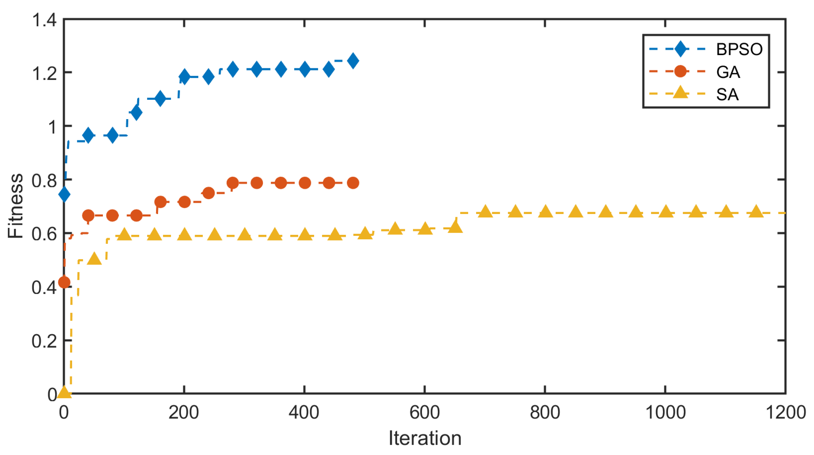
Here, we use three algorithms, including binary particle swarm optimization (BPSO), genetic algorithm (GA), and simulated annealing (SA), to conduct the inverse design of the dual-band antenna and make a comparison of their performance. During the optimization, we adopt the fitness function as the objective function:

$$F(D)=\underset{\mathrm{Primary} \mathrm{resonance} \mathrm{constraint} }{\underbrace{w_1\sum _{i=1}^2 1- \mathrm{m}\mathrm{a}\mathrm{x}\left(S\left[f_i\right]-\mathrm{0.1,0}\right)}}+\underset{\mathrm{Weighted} \mathrm{bandwidth} \mathrm{constraint} }{\underbrace{w_2\sum _{i=1}^2 \sum _{k=1}^n W\left(f_k\mid f_i\right)\cdot (1-S\left[f_k\right])}}+\underset{\mathrm{Resonance} \mathrm{penalty} }{\underbrace{\lambda \cdot I( \mathrm{Noresonance} )}}$$

where the Gaussian weighting kernel is defined as follows:

$$W\left(f_k\mid f_i\right)=e^{-{\displaystyle \frac{{\left(f_k-f_i\right)}^2}{2{\sigma }^2}}}$$

with $\sigma$ controlling the decay rate of the weighting coefficients. The indicator function $I(\cdot )$ returns to 1 if resonance is detected, and 0 otherwise.

Figure 7 depicts the workflow of our proposed inverse design framework based on pre-trained CNN. The optimization algorithm generates an initial pixelated structure (binary matrix). This structure is input into the pre-trained CNN, which predicts the corresponding S-parameters. Then the predicted S-parameters are compared against the target values to compute the fitness function F(D). If the fitness function does not converge, the optimization algorithm updates the structure, and previous steps are repeated. The process terminates when the fitness function meets the convergence criterion.

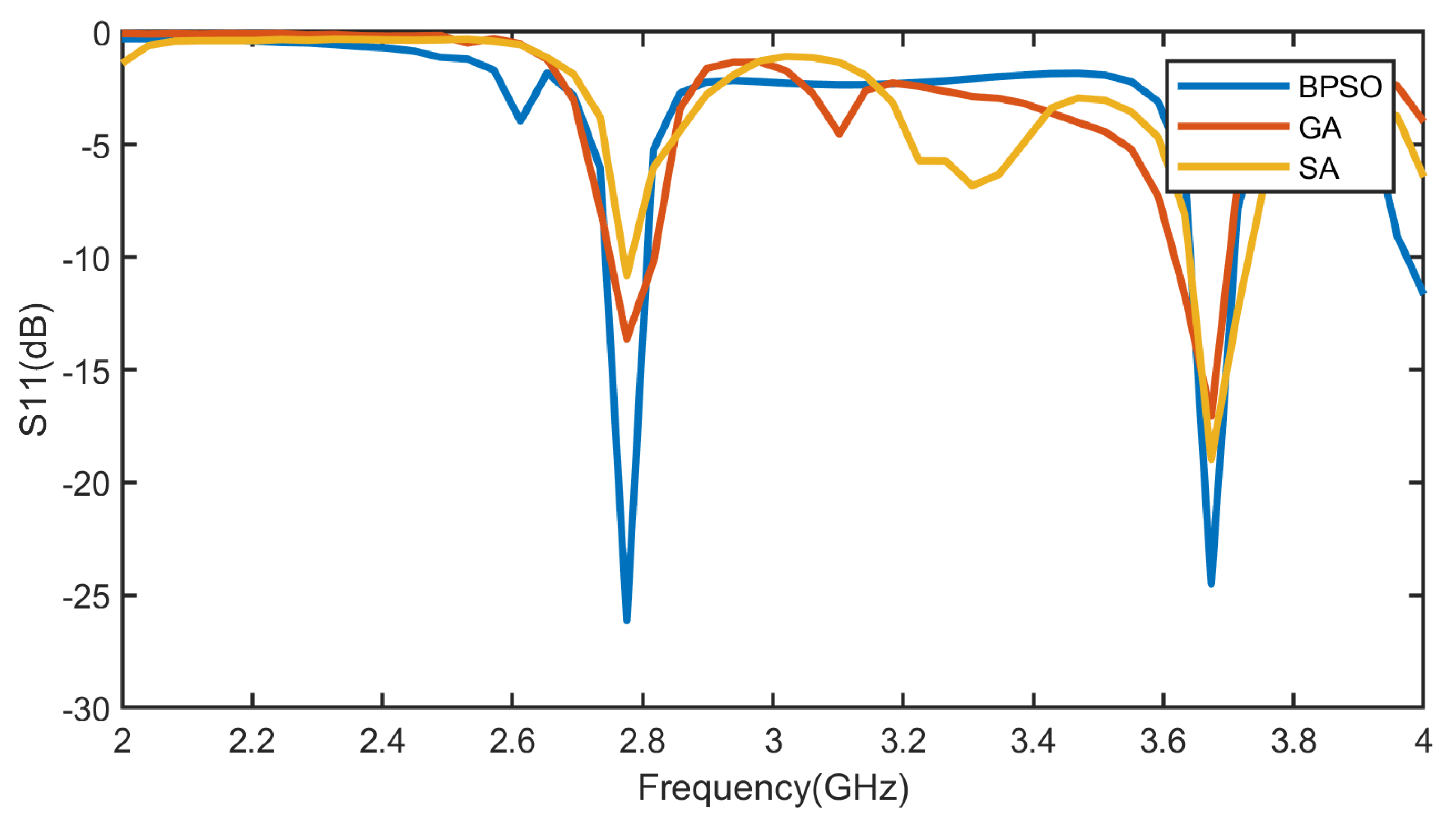
Figure 8 shows the variation in optimal fitness with iteration count for the three algorithms. As can be seen from the figure, the BPSO requires the fewest iterations to achieve the best results. Figure 9 compares the reflection coefficients of antennas optimized by the three algorithms after the same number of iterations. The figure demonstrates that the BPSO can find better solutions. We also conducted experiments varying three weight coefficients (w₁, w₂, λ) in the fitness function of BPSO, visualizing their effects on convergence speed and solution quality, as shown in Figure 10. The three weights have a common influence on the fitness function. When the weight value is too small, as shown in the cases of w₁ = 0.1, w₂ = 0.1, and λ = 0.1, the convergence speed is very slow, and the solution quality is also the worst. When the weight values increase to 0.2, the convergence speed is the fastest and the solution quality is also the best. Continuing to increase the weight value will reduce the convergence speed and the solution quality.

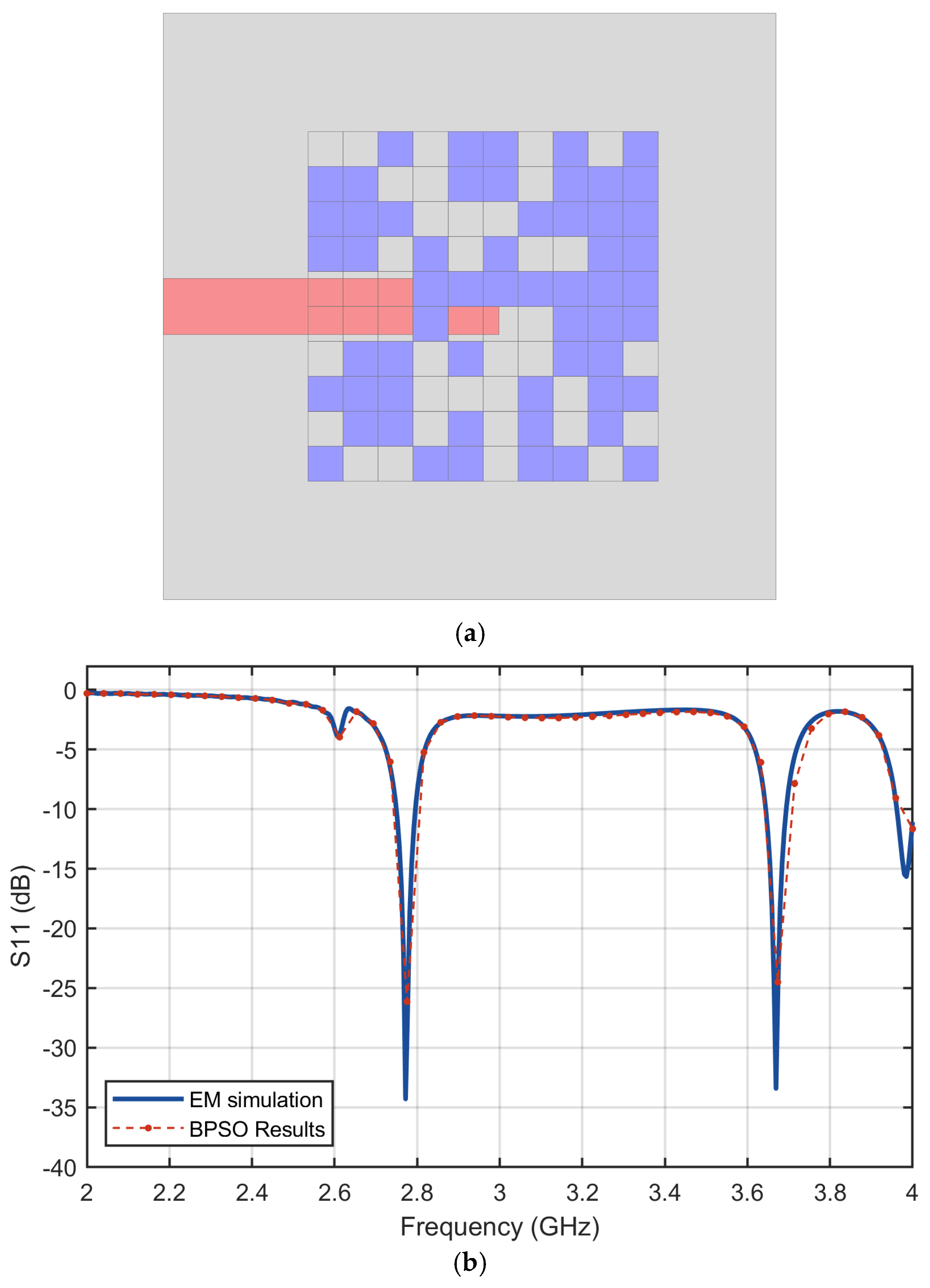
Figure 11a shows the antenna structure generated by the proposed inverse design approach using BPSO. Figure 11b plots the reflection coefficients of the antenna predicted by CNN and the value from the full-wave simulation result from CST. Good agreement is found in the figure, which demonstrates that the proposed approach can design the antenna with a small error in terms of performance.

The antenna radiation patterns are shown in Figure 12. The simulated gains of the antenna are 7.07 dBi and 6.85 dBi at 2.8 GHz and 3.7 GHz, respectively. Since the dielectric loss is not considered in the simulation, the antenna realizes a high efficiency of 95.3% and 98.8% at 2.8 GHz and 3.7 GHz, respectively. At 2.8 GHz, the radiation pattern exhibits relatively regular characteristics, whereas at 3.7 GHz, the pattern shows reduced radiation power at θ = 0°. This behavior arises because the antenna operates in a high-order mode at 3.7 GHz, inducing reverse current flow within the patch. This phenomenon disrupts the coherent radiation mechanism, leading to the observed null in the boresight direction (θ = 0°). The gain and efficiency of our BPSO-CNN-designed antennas are comparable to those of conventional methods. However, a notable difference lies in the regularity of the radiation pattern. Unlike traditional designs with symmetric geometries, our method intentionally relaxes shape constraints to prioritize S₁₁ optimization. This results in irregular radiation patterns due to the pixelated, non-symmetrical geometries generated by the inverse design process.

4. Discussion of Methodology

The current CNN is intentionally trained on a specific configuration to validate the inverse design framework, but its extension to broader scenarios involves trade-offs and architectural considerations. Higher resolutions (e.g., 20 × 20) can enhance design precision by capturing finer geometric details, but they also increase input dimensionality and computational complexity, potentially slowing down electromagnetic simulations during training. The 10 × 10 grid balances accuracy and efficiency for proof-of-concept validation. In addition, the model currently lacks the explicit encoding of frequency and substrate parameters (thickness, εᵣ), limiting its ability to generalize to new bands or materials. In future work, we plan to develop a multi-modal neural network that incorporates frequency values and substrate properties as additional input channels alongside the pixel grid. This approach would enable the model to learn frequency- and material-dependent electromagnetic patterns, extending its applicability to diverse design requirements.

Since CNN training only uses S₁₁ as an output, the current design method cannot guarantee the antenna’s radiation characteristics, such as radiation patterns, gains, polarization, etc. In our future work, we will redesign the neural network to address this issue by incorporating the antenna’s radiation characteristics into the CNN’s output. This way, we can add explicit constraints on radiation performance within the inverse design algorithm, ensuring that optimized antennas meet radiation requirements.

Given the maturity of MATLAB-CST co-simulation interfaces, the simulation results from CST can be directly utilized as fitness values for structural optimization, bypassing the machine learning surrogate model. However, our ML surrogate model has higher computational efficiency than the MATLAB-CST co-simulation method. Notably, empirical tests confirm that on identical hardware, MATLAB-CST co-simulation requires 12.5 h for 500 optimization iterations, while the CNN surrogate model completes the same task in just 30 min, an increase in speed of 25 times that makes large-scale inverse design feasible. This performance gap underscores the ML component’s necessity in balancing accuracy and computational feasibility for large-scale inverse design.

5. Conclusions

This paper presents a novel inverse design framework for microstrip antennas, which integrates pixelated modeling, CNN-based S₁₁ prediction, and BPSO. By discretizing the radiating patch into a 10 × 10 binary matrix, it expands the design space exponentially. The CNN forward model is trained using 150,000 datasets, and it can accurately predict S₁₁ with an RMSE of 0.35, an MAE of 0.28, and an R² of 0.94. Three algorithms, BPSO, GA, and SA, are employed for the inverse design of dual-band (2.8/3.7 GHz) antenna. The experimental results demonstrate that BPSO converges faster and achieves higher design accuracy. The S11 values predicted by the CNN are in good agreement with the simulated results obtained from CST full-wave simulation. Moreover, the radiation patterns remain stable at the two operating frequencies. The proposed deep-CNN-based inverse design approach holds great promise for applications in high-efficiency automated antenna design.

References

- Chen, F.-C.; Liang, Y.-Z.; Zeng, W.-F.; Xiang, K.-R. A Series-Fed Slant-Polarized Microstrip Patch Antenna Array. IEEE Trans. Antennas Propag. 2024, 72, 5367–5372. [Google Scholar] [CrossRef]
- Shi, R.; He, Y.; Wan, Z.; Shi, J.; Sun, H. Simple E-Plane Decoupling Structure Using Embedded Mushroom Element for Wide-Angle Scanning Linear Microstrip Phased Arrays. IEEE Antennas Wirel. Propag. Lett. 2025, 24, 339–343. [Google Scholar] [CrossRef]
- Sun, G.-H.; Wong, H. A Hollow-Waveguide-Fed Planar Wideband Patch Antenna Array for Terahertz Communications. IEEE Trans. Terahertz Sci. Technol. 2023, 13, 10–19. [Google Scholar] [CrossRef]
- Chhaule, N.; Koley, C.; Mandal, S.; Onen, A.; Ustun, T.S. A Comprehensive Review on Conventional and Machine Learning-Assisted Design of 5G Microstrip Patch Antenna. Electronics 2024, 13, 3819. [Google Scholar] [CrossRef]
- Ou, N.; Wu, X.; Xu, K.; Sun, F.; Yu, T.; Luan, Y. Wideband, Dual-Polarized Patch Antenna Array Fed by Novel, Differentially Fed Structure. Electronics 2024, 13, 1382. [Google Scholar] [CrossRef]
- Ji, Z.; Sun, G.-H.; Wong, H. A Wideband Circularly Polarized Complementary Antenna for Millimeter-Wave Applications. IEEE Trans. Antennas Propag. 2022, 70, 2392–2400. [Google Scholar] [CrossRef]
- Yi, X.; Wong, H. Wideband and High-Gain Substrate Integrated Folded Horn Fed Open Slot Antenna. IEEE Trans. Antennas Propag. 2022, 70, 2602–2612. [Google Scholar] [CrossRef]
- Karahan, E.A.; Gupta, A.; Khankhoje, U.K.; Sengupta, K. Deep Learning-Based Inverse Design for Planar Antennas at RF and Millimeter-Wave. In Proceedings of the 2022 IEEE International Symposium on Antennas Propagation and USNC-URSI Radio Science Meeting (AP-S/URSI), Piscataway, NJ, USA, 10–15 July 2022. [Google Scholar]
- Jacobs, J.P. Convolutional Neural-Network Regression for Dual-Band Pixelated Microstrip Antennas. IEEE Antennas Wirel. Propag. Lett. 2021, 20, 2417–2421. [Google Scholar] [CrossRef]
- Noakoasteen, O.; Vijayamohan, J.; Gupta, A. GAN-Based Synthetic Data Generation for Antenna Design. IEEE Open J. Antennas Propag. 2022, 3, 488–494. [Google Scholar] [CrossRef]
- Misilmani, H.M.E.; Naous, T. Machine Learning in Antenna Design: A Comprehensive Overview. IEEE Access 2023, 11, 103890–103915. [Google Scholar]
- Du, Z.; Wang, K.; Ruan, X.; Sun, G. An Optimization Design Method for Dual-Band and Wideband Patch Filtering Power Dividers. Electronics 2024, 13, 528. [Google Scholar] [CrossRef]
- Wu, Q.; Chen, W.; Yu, C.; Wang, H.; Hong, W. Machine—Learning—Assisted Optimization for Antenna Geometry Design. IEEE Trans. Antennas Propag. 2024, 72, 2083–2095. [Google Scholar] [CrossRef]
- Xiao, L.-Y.; Shao, W.; Jin, F.-L.; Wang, B.-Z.; Liu, Q.H. Inverse Artificial Neural Network for Multiobjective Antenna Design. IEEE Trans. Antennas Propag. 2021, 69, 6651–6659. [Google Scholar] [CrossRef]
- Karahan, E.A.; Liu, Z.; Sengupta, K. Deep—Learning—Based Inverse—Designed Millimeter—Wave Passives and Power Amplifiers. IEEE J. Solid-State Circuits 2023, 58, 3074–3088. [Google Scholar] [CrossRef]
- Gupta, A.; Karahan, E.A.; Bhat, C.; Sengupta, K.; Khankhoje, U.K. Tandem Neural Network Based Design of Multiband Antennas. IEEE Trans. Antennas Propag. 2023, 71, 6308–6317. [Google Scholar] [CrossRef]
- Goyal, P.; Dollár, P.; Girshick, R.; Noordhuis, P.; Wesolowski, L.; Kyrola, A.; He, K. Accurate, Large Minibatch SGD: Training ImageNet in 1 Hour. arXiv 2017, arXiv:1706.02677. [Google Scholar]