

Signal-Specific and Signal-Independent Features for Real-Time Beat-by-Beat ECG Classification with AI for Cardiac Abnormality Detection


Abstract
1. Introduction
- We fused 159 automatically extracted signal-independent (SI) descriptors with 28 handcrafted signal-specific (SS) morphology metrics and then ranked them with a one-way ANOVA filter.
- ANOVA is selected over Mutual Information and ReliefF because it is hyperparameter-free, fully deterministic, and makes on-device feature selection feasible and reproducible.
- A 128-layer CNN driven by the fused ANOVA ranked feature set achieves 100% accuracy.
- We contrast our results with recent CNN, hybrid CNN–Transformer models, and self-supervised methods, highlighting that our approach uniquely combines feature-level interpretability with a full power profile while matching or exceeding their accuracy on a stricter seven-category inter-patient split.
2. Materials and Methods
2.1. Data Preparation
2.2. ECG Signal Preprocess
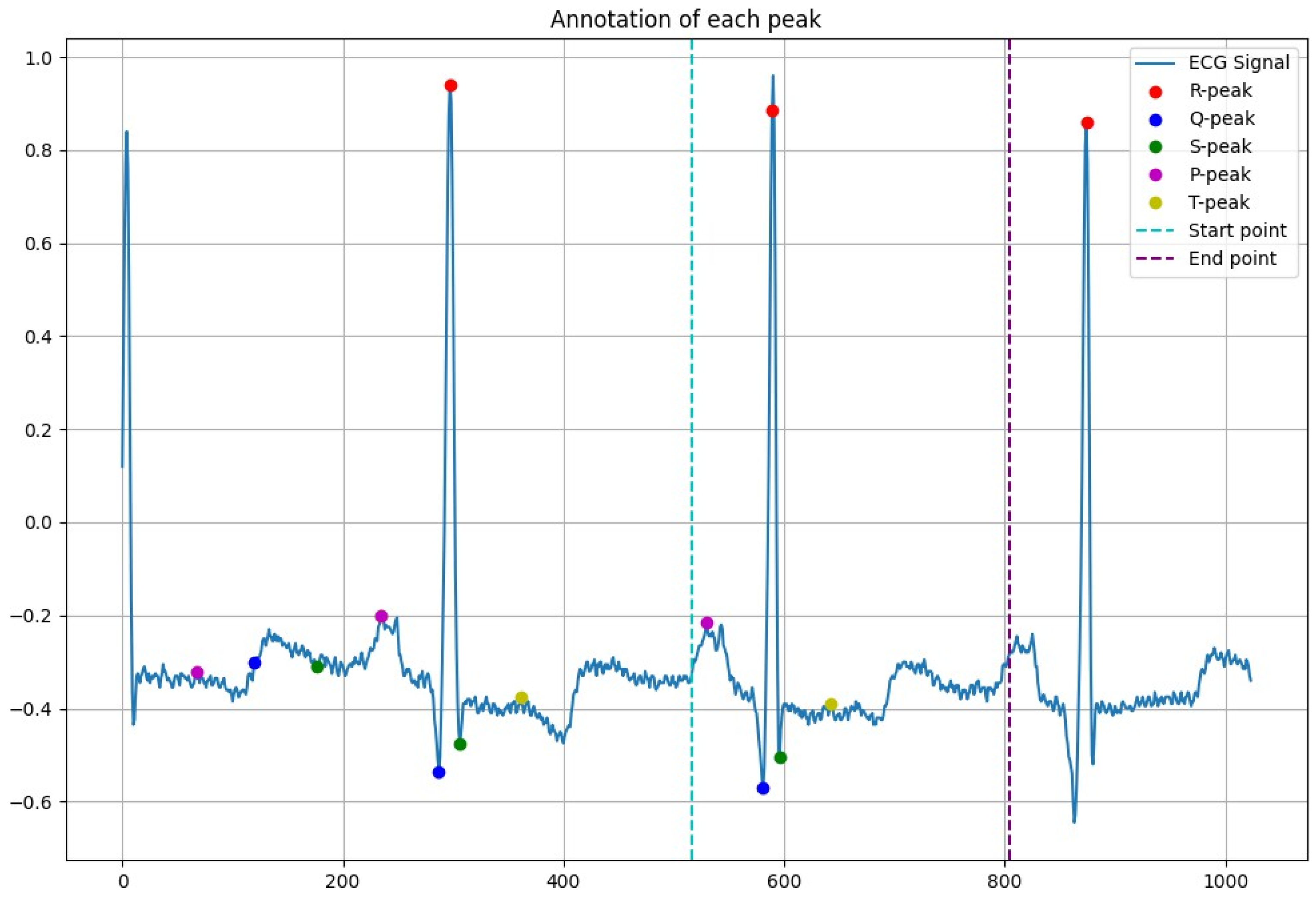
2.3. Peak Detection
| Algorithm 1: Find ECG peaks. |
|
2.4. Feature Extraction and Selection
2.4.1. ANOVA Algorithm
2.4.2. Comparison with Other Filters and Feature-Set Stability
2.5. Classification
- Layers: {32, 64, 128, 256},
- Units/filters per layer: {16, 32, 64},
- Optimizer: {Adam, RMSProp} The best configuration for each architecture (e.g., 128-layer CNN with 32 filters, 0.2 dropout, Adam 5 × 10⁻⁴) was selected based on validation F1-score.
2.6. Performance
3. Experimental Results
3.1. Peak Detection
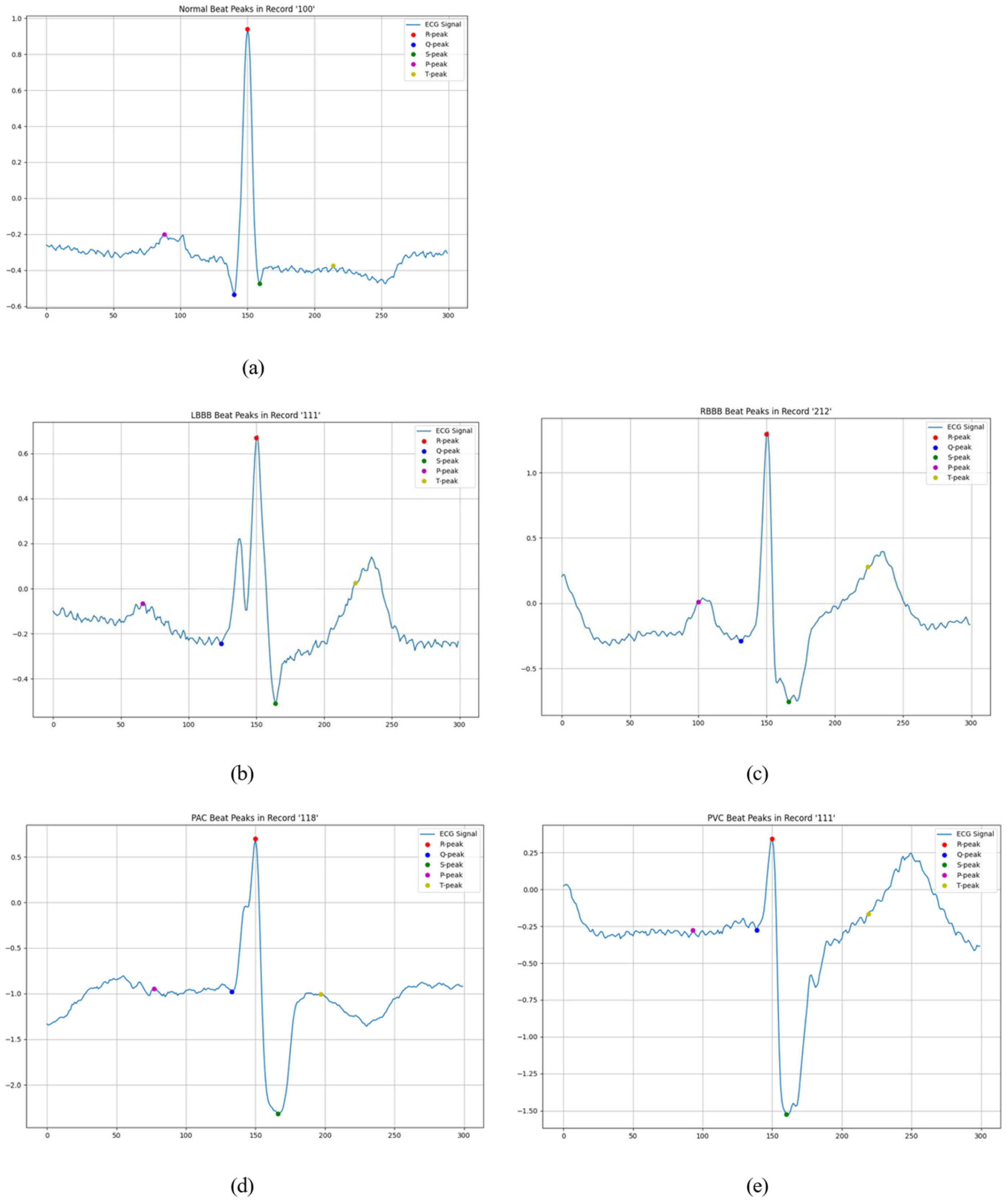
3.2. Beat Detection
3.3. Feature Extraction, Selection and Ranking
3.3.1. Signal-Specific Feature
3.3.2. Signal-Independent Feature
3.4. Classification
3.4.1. Before Feature Ranking
3.4.2. After Feature Ranking
3.5. Power Consumption
4. Conclusions
5. Future Work and Clinical Implications
Author Contributions
Funding
Data Availability Statement
Conflicts of Interest
Abbreviations
| AI | Artificial intelligence |
| ANOVA | Analysis of variance |
| CNN | Convolutional neural network |
| DL | Deep learning |
| ECG | Electrocardiogram |
| IoT | Internet of Things |
| KNN | k-Nearest Neighbor |
| LSTM | Long short-term memory network |
| ML | Machine learning |
| RF | Random forest |
| SVM | Support-vector machine |
| TSFEL | Time-Series Feature Extraction Library |
Appendix A
Appendix A.1. Signal-Specific Feature

| Feature Type | Description |
|---|---|
| Signal-specific feature (Total of 28) | |
| 7 amplitude features | |
| Q, S, T, R peak | Peak of Q, S, T, R |
| QRS pos | Mean slope of the waveform at QRS position |
| QT, RR | Length of QT and RR |
| 6 frequency features | |
| fQ, fR, fS, fT | Sampling frequency of Q, R, S, T |
| instantHR duration of consecutive cardiac cycles is constant. | Instantaneous heart rate (HR). The number of heart beats in one minute when the |
| HR | Heart rate (HR). The number of cardiac cycle (RR interval) per minute. |
| 15 statistic features | |
| mfR, mfQ, mfS, mfT, mQT | Mean peak value of R, Q, S, T, and QT |
| meanLF range | Mean value of low frequency power (LF); Frequency activity in the 0.04–0.15 Hz |
| meanHF range | Mean value of high frequency power (HF); Frequency activity in the 0.15–0.40 Hz |
| LF/HF | The ration of low frequency power (LF)to high frequency power (HF) |
| mVLF | Mean of very low frequency (VLF) |
| LFnu | Relative power of the low frequency band (0.04–0.15 Hz) in normal units |
| HFnu | Relative power of the high frequency band (0.15–0.40 Hz) in normal units |
| maxF | Maximum frequency |
| pnn50 than 50 milliseconds per hour | The average number of consecutive normal sinus (NN) intervals that change more |
| rmssd | The root mean square of successive difference between normal heartbeats |
| s_wt transforms (DWT) of a given signal | Stationary Wavelet Transform (SWT) Computes all decimated discrete wavelet |
Appendix A.2. Signal-Independent Feature
| Feature Type | Summary |
|---|---|
| Signal-independent feature | Total of 159 features be extracted |
| Time series feature extraction library (TSFEL) | Absolute_energy, 0_Area under the curve, 0_Autocorrelation, 0_Centroid, 0_ECDF Percentile Count_0, 0_ECDF Percentile Count_1, 0_ECDF Percentile_0, 0_ECDF Percentile_1, ECDF_0, ECDF_1, 0_ECDF_2, 0_ECDF_3, 0_ECDF_4, 0_ECDF_5, 0_ECDF_6, 0_ECDF_7, 0_ECDF_8, 0_ECDF_9, 0_Entropy, 0_FFT mean coefficient_0, 0_FFT mean coefficient_1, 0_FFT mean coefficient_10, 0_FFT mean coefficient_11, 0_FFT mean coefficient_12, 0_FFT mean coefficient_13, 0_FFT mean coefficient_14, 0_FFT mean coefficient_15, 0_FFT mean coefficient_16, 0_FFT mean coefficient_17, 0_FFT mean coefficient_18, 0_FFT mean coefficient_19, 0_FFT mean coefficient_2, 0_FFT mean coefficient_20, 0_FFT mean coefficient_21, 0_FFT mean coefficient_22, 0_FFT mean coefficient_23, 0_FFT mean coefficient_24, 0_FFT mean coefficient_25, 0_FFT mean coefficient_3, 0_FFT mean coefficient_4, 0_FFT mean coefficient_5, 0_FFT mean coefficient_6, 0_FFT mean coefficient_7, 0_FFT mean coefficient_8, 0_FFT mean coefficient_9, 0_Fundamental frequency, 0_Histogram_0, 0_Histogram_1, 0_Histogram_2, 0_Histogram_3, 0_Histogram_4, 0_Histogram_5, 0_Histogram_6, 0_Histogram_7, 0_Histogram_8, 0_Histogram_9, 0_Human range energy, 0_Interquartile range, 0_Kurtosis, 0_LPCC_0, 0_LPCC_1, 0_LPCC_10, 0_LPCC_11, 0_LPCC_2, 0_LPCC_3, 0_LPCC_4, 0_LPCC_5, 0_LPCC_6, 0_LPCC_7, 0_LPCC_8, 0_LPCC_9, 0_MFCC_0, 0_MFCC_1, 0_MFCC_10, 0_MFCC_11, 0_MFCC_2, 0_MFCC_3, 0_MFCC_4, 0_MFCC_5, 0_MFCC_6, 0_MFCC_7, 0_MFCC_8, 0_MFCC_9, 0_Max, 0_Max, power spectrum, 0_Maximum frequency, 0_Mean, 0_Mean absolute deviation, 0_Mean absolute diff, 0_Mean diff, 0_Median, 0_Median absolute deviation, 0_Median absolute diff, 0_Median diff, 0_Median frequency, 0_Min, 0_Negative turning points, 0_Neighbourhood peaks, 0_Peak to peak distance, 0_Positive turning points, 0_Power bandwidth, 0_Root mean square, 0_Signal distance, 0_Skewness, 0_Slope, 0_Spectral centroid, 0_Spectral decrease, 0_Spectral distance, 0_Spectral entropy, 0_Spectral kurtosis, 0_Spectral positive turning points, 0_Spectral roll-off, 0_Spectral roll-on, 0_Spectral skewness, 0_Spectral slope, 0_Spectral spread, 0_Spectral variation, 0_Standard deviation, 0_Sum absolute diff, 0_Total energy 0_Variance, 0_Wavelet absolute mean_0, 0_Wavelet absolute mean_1, 0_Wavelet absolute mean_2, 0_Wavelet absolute mean_3, 0_Wavelet absolute mean_4, 0_Wavelet absolute mean_5, 0_Wavelet absolute mean_6, 0_Wavelet absolute mean_7, 0_Wavelet absolute mean_8, 0_Wavelet energy_0, 0_Wavelet energy_1, 0_Wavelet energy_2, 0_Wavelet energy_3, 0_Wavelet energy_4, 0_Wavelet energy_5, 0_Wavelet energy_6, 0_Wavelet energy_7, 0_Wavelet energy_8, 0_Wavelet entropy, 0_Wavelet standard deviation_0, 0_Wavelet standard deviation_1, 0_Wavelet standard deviation_2, 0_Wavelet standard deviation_3, 0_Wavelet standard deviation_4, 0_Wavelet standard deviation_5, 0_Wavelet standard deviation_6, 0_Wavelet standard deviation_7, 0_Wavelet standard deviation_8, Wavelet_variance_0, Wavelet_variance_1, 0_Wavelet variance_2, 0_Wavelet variance_3, 0_Wavelet variance_4, 0_Wavelet variance_5, 0_Wavelet variance_6, 0_Wavelet variance_7, 0_Wavelet variance_8, Zero crossing rate. |
| ANOVA algorithm | Total of 99 features be selected |
| ‘0_Histogram_6’, ‘0_Histogram_2’, ‘0_Histogram_8’, ‘0_Histogram_3’, ‘0_Spectral roll-on’, ‘Zero crossing rate’, ‘0_Positive turning points’, ‘0_Spectral spread’, ‘0_Histogram_5’, ‘0_Spectral centroid’, ‘0_ECDF Percentile_0’, ‘0_Histogram_4’, ‘0_LPCC_1’, ‘0_Median’, ‘0_Power bandwidth’, ‘0_Negative turning points’, ‘0_Maximum frequency’, ‘0_LPCC_6’, ‘0_Mean’, ‘0_Spectral entropy’, ‘0_Spectral skewness’, ‘0_MFCC_11’, ‘0_MFCC_2’, ‘0_MFCC_8’, ‘0_Interquartile range’, ‘0_LPCC_4’, ‘0_LPCC_5’, ‘0_MFCC_1’, ‘0_Skewness’, ‘0_Median frequency’, ‘0_Histogram_7’, ‘0_Human range energy’, ‘0_ECDF Percentile_1’, ‘0_MFCC_9’, ‘0_Neighbourhood peaks’, ‘Absolute_energy’, ‘0_Total energy’, ‘0_MFCC_0’, ‘0_Spectral kurtosis’, ‘0_LPCC_3’, ‘0_LPCC_10’, ‘0_MFCC_5’, ‘0_Sum absolute diff’, ‘0_Wavelet variance_2’, ‘Wavelet_variance_1’, ‘0_Signal distance’, ‘0_Histogram_9’, ‘0_Spectral variation’, ‘0_MFCC_3’, ‘0_Wavelet variance_8’, ‘0_MFCC_7’, ‘0_Wavelet variance_3’, ‘0_Histogram_0’, ‘0_Spectral positive turning points’, ‘Wavelet_variance_0’, ‘0_MFCC_10’, ‘0_Wavelet energy_1’, ‘0_MFCC_6’, ‘0_Wavelet standard deviation_1’, ‘0_ECDF Percentile Count_1’, ‘0_ECDF Percentile Count_0’, ‘0_Wavelet absolute mean_7’, ‘0_Wavelet energy_0’, ‘0_Wavelet standard deviation_0’, ‘0_Spectral decrease’, ‘0_Wavelet absolute mean_8’, ‘0_Wavelet absolute mean_6’, ‘0_MFCC_4’, ‘0_Wavelet energy_2’, ‘0_Wavelet variance_7’, ‘0_Wavelet standard deviation_2’, ‘0_Wavelet variance_4’, ‘0_Wavelet absolute mean_5’, ‘0_Wavelet energy_3’, ‘0_Wavelet standard deviation_3’, ‘0_Spectral distance’, ‘0_Mean absolute deviation’, ‘0_Wavelet energy_8’, ‘0_Wavelet standard deviation_4’, ‘0_Wavelet energy_4’, ‘0_Root mean square’, ‘0_Wavelet standard deviation_8’, ‘0_Max’, ‘0_Wavelet standard deviation_5’, ‘0_Fundamental frequency’, ‘0_Wavelet variance_5’, ‘0_Wavelet energy_5’, ‘0_Wavelet variance_6’, ‘0_Wavelet energy_7’, ‘0_Variance’, ‘0_Peak to peak distance’, ‘0_Kurtosis’, ‘0_Standard deviation’, ‘0_Min’, ‘0_Wavelet standard deviation_7’, ‘0_Wavelet standard deviation_6’, ‘0_Histogram_1’, ‘0_Wavelet energy_6’. | |
| Top 15 ranked features | 0_Wavelet standard deviation_5, 0_Fundamental frequency, 0_Wavelet variance_5, 0_Wavelet energy_5, 0_Wavelet variance_6, 0_Wavelet energy_7, 0_Variance, 0_Peak to peak distance, 0_Kurtosis, 0_Standard deviation, 0_Min, 0_Wavelet standard deviation_7, 0_Wavelet standard deviation_6, 0_Histogram_1, 0_Wavelet energy_6. |
References
- Rahman, M.; Hewitt, R.; Morshed, B.I. Design and Packaging of a Custom Single-lead Electrocardiogram (ECG) Sensor Embedded with Wireless Transmission. In Proceedings of the 2023 IEEE 16th Dallas Circuits and Systems Conference (DCAS), Denton, TX, USA, 14–16 April 2023; pp. 1–4. [Google Scholar] [CrossRef]
- Momota, M.M.R.; Morshed, B.I. ML algorithms to estimate data reliability metric of ECG from inter-patient data for trustable AI-based cardiac monitors. Smart Health 2022, 26, 100350. [Google Scholar] [CrossRef]
- Saritha, C.; Sukanya, V.; Murthy, Y. ECG Signal Analysis Using Wavelet Transforms. Bulg. J. Phys. 2008, 35, 68–77. [Google Scholar]
- Drew, B.J.; Pelter, M.M.; Wung, S.-F.; Adams, M.G.; Taylor, C.; Evans, G.T.; Foster, E. Accuracy of the EASI 12-lead electrocardiogram compared to the standard 12-lead electrocardiogram for diagnosing multiple cardiac abnormalities. J. Electrocardiol. 1999, 32 (Suppl. 1), 38–47. [Google Scholar] [CrossRef] [PubMed]
- Momota, M.M.R.; Morshed, B.I. Inkjet Printed Flexible Electronic Dry ECG Electrodes on Polyimide Substrates Using Silver Ink. In Proceedings of the 2020 IEEE International Conference on Electro Information Technology (EIT), Chicago, IL, USA, 31 July–1 August 2020; pp. 464–468. [Google Scholar] [CrossRef]
- Auer, R.; Bauer, D.C.; Marques-Vidal, P.; Butler, J.; Min, L.J.; Cornuz, J.; Satterfield, S.; Newman, A.B.; Vittinghoff, E.; Rodondi, N.; et al. Association of major and minor ECG abnormalities with coronary heart disease events. JAMA 2012, 307, 1497–1505. [Google Scholar]
- Padmavathi, K.; Ramakrishna, K.S. Classification of ECG signal during atrial fibrillation using autoregressive modeling. Procedia Comput. Sci. 2015, 46, 53–59. [Google Scholar] [CrossRef]
- Çınar, A.; Tuncer, S.A. Classification of normal sinus rhythm, abnormal arrhythmia and congestive heart failure ECG signals using LSTM and hybrid CNN-SVM deep neural networks. Comput. Methods Biomech. Biomed. Eng. 2021, 24, 203–214. [Google Scholar] [CrossRef]
- Kaya, Y.; Pehlivan, H. Classification of premature ventricular contraction in ECG. Int. J. Adv. Comput. Sci. Appl. 2015, 6, 34–40. [Google Scholar] [CrossRef]
- ITsai, H.; Morshed, B.I. Beat-by-Beat Classification of ECG Signals Using Machine Learning Algorithms to Detect PVC Beats for Real-time Predictive Cardiac Health Monitoring. In Proceedings of the 2022 IEEE International Conference on Bioinformatics and Biomedicine (BIBM), Las Vegas, NV, USA, 6–8 December 2022; pp. 1751–1754. [Google Scholar] [CrossRef]
- Baig, M.M.; Gholamhosseini, H. Smart health monitoring systems: An overview of design and modeling. J. Med. Syst. 2013, 37, 9898. [Google Scholar] [CrossRef]
- Abdul-Qawy, A.S.; Pramod, P.J.; Magesh, E.; Srinivasulu, T. The internet of things (iot): An overview. Int. J. Eng. Res. Appl. 2015, 5, 71–82. [Google Scholar]
- Utsha, U.T.; Hua Tsai, I.; Morshed, B.I. A Smart Health Application for Real-Time Cardiac Disease Detection and Diagnosis Using Machine Learning on ECG Data. In Internet of Things. Advances in Information and Communication Technology. IFIPIoT 2023. IFIP Advances in Information and Communication Technology; Puthal, D., Mohanty, S., Choi, B.Y., Eds.; Springer: Cham, Switzerland, 2024; Volume 683. [Google Scholar] [CrossRef]
- Wan, J.; AAH Al-awlaqi, M.; Li, M.; O’Grady, M.; Gu, X.; Wang, J.; Cao, N. Wearable IoT enabled real-time health monitoring system. EURASIP J. Wirel. Commun. Netw. 2018, 2018, 298. [Google Scholar] [CrossRef]
- Mouha, R.A. Internet of things (IoT). J. Data Anal. Inf. Process. 2021, 9, 77–101. [Google Scholar]
- Yu, Z.; Xu, M.; Gao, Z. Biomedical image segmentation via constrained graph cuts and pre-segmentation. In Proceedings of the 2011 Annual International Conference of the IEEE Engineering in Medicine and Biology Society, Boston, MA, USA, 30 August–3 September 2011; pp. 5714–5717. [Google Scholar] [CrossRef]
- Ihsanto, E.; Ramli, K.; Sudiana, D.; Gunawan, T.S. An efficient algorithm for cardiac arrhythmia classification using ensemble of depthwise separable convolutional neural networks. Appl. Sci. 2020, 10, 483. [Google Scholar] [CrossRef]
- Tsai, I.H.; Morshed, B.I. Scalable and Upgradable AI for Detected Beat-By-Beat ECG Signals in Smart Health. In Proceedings of the 2023 IEEE World AI IoT Congress (AIIoT), Seattle, WA, USA, 7–10 June 2023; pp. 0409–0414. [Google Scholar]
- Peimankar, A.; Puthusserypady, S. DENS-ECG: A deep learning approach for ECG signal delineation. Expert Syst. Appl. 2021, 165, 113911. [Google Scholar] [CrossRef]
- Kotorov, R.; Chi, L.; Shen, M. Personalized monitoring model for electrocardiogram signals: Diagnostic accuracy study. JMIR Biomed. Eng. 2020, 5, e24388. [Google Scholar] [CrossRef]
- Xu, M.; Yu, Z. 3D image segmentation based on feature-sensitive and adaptive tetrahedral meshes. In Proceedings of the 2016 IEEE International Conference on Image Processing (ICIP), Phoenix, AZ, USA, 25–28 September 2016; pp. 854–858. [Google Scholar] [CrossRef]
- Tsai, I.H.; Morshed, B.I. Beat-by-beat Classification of ECG Signals with Machine Learning Algorithm for Cardiac Episodes. In Proceedings of the 2022 IEEE International Conference on Electro Information Technology (eIT), Mankato, MN, USA, 19–21 May 2022; pp. 311–314. [Google Scholar]
- Raza, A.; Tran, K.P.; Koehl, L.; Li, S. Designing ecg monitoring healthcare system with federated transfer learning and explainable ai. Knowl.-Based Syst. 2022, 236, 107763. [Google Scholar] [CrossRef]
- Sraitih, M.; Jabrane, Y.; Hajjam El Hassani, A. An automated system for ECG arrhythmia detection using machine learning techniques. J. Clin. Med. 2021, 10, 5450. [Google Scholar] [CrossRef]
- Tsai, I.H.; Morshed, B.I. Detecting PVC Beats by Beat-by-beat Analysis of ECG Signals Using Machine Learning Classifiers for Real-time Predictive Cardiac Health Monitoring. In Proceedings of the 2022 IEEE 13th Annual Ubiquitous Computing, Electronics & Mobile Communication Conference (UEMCON), New York, NY, USA, 26–29 October 2022; pp. 0355–0361. [Google Scholar]
- Torres-Soto, J.; Ashley, E.A. Multi-task deep learning for cardiac rhythm detection in wearable devices. Npj Digit Med. 2020, 3, 116. [Google Scholar] [CrossRef]
- Kim, S.; Chon, S.; Kim, J.K.; Kim, J.; Gil, Y.; Jung, S. Lightweight Convolutional Neural Network for Real-Time Arrhythmia Classification on Low-Power Wearable Electrocardiograph. In Proceedings of the 2022 44th Annual International Conference of the IEEE Engineering in Medicine & Biology Society (EMBC), Glasgow, Scotland, UK, 11–15 July 2022; pp. 1915–1918. [Google Scholar] [CrossRef] [PubMed]
- Contoli, C.; Freschi, V.; Lattanzi, E. Energy-aware human activity recognition for wearable devices: A comprehensive review. Pervasive Mob. Comput. 2024, 104, 101976. [Google Scholar] [CrossRef]
- Vashishth, T.K.; Sharma, V.; Sharma, K.K.; Kumar, B.; Chaudhary, S.; Panwar, R. Chapter 10 Enhancing biomedical signal processing with machine learning: A comprehensive review. In Digital Transformation in Healthcare 5.0: Volume 1: IoT, AI and Digital Twin; Malviya, R., Sundram, S., Dhanaraj, R.K., Kadry, S., Eds.; De Gruyter: Berlin, Germany; Boston, MA, USA, 2024; pp. 277–306. [Google Scholar] [CrossRef]
- Kwon, S.H.; Dong, L. Flexible sensors and machine learning for heart monitoring. Nano Energy 2022, 102, 107632. [Google Scholar] [CrossRef]
- Gupta, U.; Paluru, N.; Nankani, D.; Kulkarni, K.; Awasthi, N. A comprehensive review on efficient artificial intelligence models for classification of abnormal cardiac rhythms using electrocardiograms. Heliyon 2024, 10, e26787. [Google Scholar] [CrossRef]
- Aminorroaya, A.; Biswas, D.; Pedroso, A.F.; Khera, R. Harnessing Artificial Intelligence for Innovation in Interventional Cardiovascular Care. J. Soc. Cardiovasc. Angiogr. Interv. 2025, 4, 102562. [Google Scholar] [CrossRef] [PubMed]
- Barandas, M.; Folgado, D.; Fernandes, L.; Santos, S.; Abreu, M.; Bota, P.; Liu, H.; Schultz, T.; Gamboa, H. Tsfel: Time series feature extraction library. SoftwareX 2020, 11, 100456. [Google Scholar] [CrossRef]
- Goldberger, A.L.; Amaral, L.A.N.; Glass, L.; Hausdorff, J.M.; Ivanov PCh Mark, R.G.; Mietus, J.E.; Moody, G.B.; Peng, C.-K.; Stanley, H.E. PhysioBank, PhysioToolkit, and PhysioNet: Components of a New Research Resource for Complex Physiologic Signals. Circulation 2000, 101, e215–e220. [Google Scholar] [CrossRef] [PubMed]
- Prakash, A.J.; Ari, S. AAMI Standard Cardiac Arrhythmia Detection with Random Forest Using Mixed Features. In Proceedings of the 2019 IEEE 16th India Council International Conference (INDICON), Rajkot, India, 13–15 December 2019; pp. 1–4. [Google Scholar]
- Pan, J.; Tompkins, W.J. A real-time QRS detection algorithm. IEEE Trans. Biomed. Eng. 1985, 32, 230–236. [Google Scholar] [CrossRef]
- Makowski, D.; Pham, T.; Lau, Z.J.; Brammer, J.C.; Lespinasse, F.; Pham, H.; Schölzel, C.; Chen, S.H.A. NeuroKit2: A Python toolbox for neurophysiological signal processing. Behav. Res. 2021, 53, 1689–1696. [Google Scholar] [CrossRef]
- St»hle, L.; Wold, S. Analysis of variance (ANOVA). Chemom. Intell. Lab. Syst. 1989, 6, 259–272. [Google Scholar] [CrossRef]


| Ref | Accuracy | Energy | ||
|---|---|---|---|---|
| Kim et al., 2025 [27] | Contribution | Lightweight CNN for real-time arrhythmia classification on low-power wearable ECG | 95% | N/R |
| Key takeaway | A 95% accuracy with 125 k parameters on a wearable patch | |||
| Relation to this study | Matches accuracy; we add feature-level interpretability and full STM32H7 power profiling | |||
| Contoli et al., 2024 [28] | Contribution | Energy-aware human-activity recognition review for wearables | N/R | Qualitative mapping only |
| Key takeaway | Maps sensor-inference energy trade-offs | |||
| Relation to this study | Our beat-level ECG study quantifies these trade-offs via real microcontroller energy measurements | |||
| Vashishth et al., 2024 [29] | Contribution | Self-supervised learning for ECG/PPG systematic review | 94% | N/R |
| Key takeaway | Highlights SSL to reduce labeling demands | |||
| Relation to this study | Our handcrafted SI + SS fusion avoids the need for large unlabeled corpora | |||
| Kwon & Dong, 2023 [30] | Contribution | Flexible sensors and ML co-design for heart monitoring | reported on custom dataset | 1335 ms |
| Key takeaway | Demonstrates hardware–software synergy | |||
| Relation to this study | We extend synergy by reporting < 25 ms inference on an off-the-shelf STM32H7 MCU | |||
| Gupta et al., 2025 [31] | Contribution | Efficient AI models for abnormal-rhythm ECG classification review | aggregated results 96–99% | 142 ms |
| Key takeaway | Advocates combining handcrafted and learned representations | |||
| Relation to this study | We operationalize this via ANOVA-ranked SI + SS feeding both ML and DL classifiers | |||
| Aminorroaya, 2024 [32] | Contribution | AI innovations in interventional cardiovascular care survey | 80–90% | N/R |
| Key takeaway | Focuses on cath-lab decision support | |||
| Relation to this study | Our work targets pre-intervention long-term rhythm surveillance via energy-constrained wearables | |||
| Our proposed method | Contribution | Edge-ready arrhythmia classifier that fuses interpretable signal-independent (SI) and signal-specific (SS) features. Two variants are benchmarked: (i) an ultra-low-power SVM and (ii) a 128-layer CNN for peak accuracy. | 100% | 9.7 mJ/23 ms |
| Key takeaway | Achieves 96.8–100% accuracy, 9.7 mJ/23 ms per beat on an STM32H7, and provides feature-level (ANOVA + SHAP) and Grad-CAM explanations—showing that handcrafted features and lightweight models can rival deeper CNNs while remaining transparent and energy-efficient. | |||
| Relation to this study | (proposed method) |
| Group Symbol | Original Symbol | Original Description | Total Beat | Training Dataset (80%) | Testing Dataset (20%) | Label |
|---|---|---|---|---|---|---|
| N Any heartbeat not categorized as S, V, F or Q | N | Normal beat (N) | 75,052 | 60,041 | 15,011 | 0 |
| L | Left Bundle branch block beat (LBBB) | 8075 | 6460 | 1615 | 1 | |
| R | Right Bundle branch block beat (RBBB) | 7259 | 5807 | 1452 | 2 | |
| e | Atrial escape beat (AE) | 16 | ||||
| j | Nodal (junctional) escape beat (NE) | 229 | ||||
| S Supraventricular ectopic beat | A | Atrial premature beat (AP) | 2546 | 2036 | 510 | 3 |
| a | Aberrated atrial premature beat (aAP) | 150 | ||||
| J | Nodal premature beat (NP) | 53 | ||||
| S | Supraventricular premature beat (SP) | 2 | ||||
| V Ventricular ectopic beat | E | Ventricular escape beat (VE) | 106 | |||
| V | Premature ventricular contraction (PVC) | 7130 | 5704 | 1426 | 4 | |
| F Fusion beat | F | Fusion of ventricular and normal beat (IVN) | 803 | 642 | 161 | 5 |
| Q Unknown beat | / | Paced beat (P) | 7028 | 5622 | 1406 | 6 |
| U | Unclassified beat (U) | 33 | 26 | 7 | ||
| f | Fusion of paced and normal beat (fPN) | 982 | 785 | 197 | ||
| Total | 109,494 | 87,123 | 21,785 |
| Peak | Formula | Search Window (Indices) | Criterion |
|---|---|---|---|
| Q | Before every RR interval, minimum between 1/8 of each R peak to R peak | minimum | |
| P | Before every R peak to Q peak, from 3/8 of RR maximum | maximum | |
| S | Before every R peak, minimum between every R peak to 1/4 of RR | minimum | |
| T | After 1/4 of R peak to R peak to the 3/8 of R peak to R peak in maximum | maximum | |
| T′ | After 1/4 of R peak to R peak to the 3/8 of R peak to R peak in minimum | reference point |
| Aspect | ANOVA (F-Test) | Mutual Information | Relief F |
|---|---|---|---|
| Statistical basis | Parametric separation of class means and variances | Non-parametric information-theoretic dependency | Instance-based nearest-neighbor relevance |
| Hyperparameters | None | Bin-size/kernel choice | k-nearest neighbors, m iterations |
| Computational cost | O(pn) simple closed-form (fast) | O(pn log n) with kernel density | O(kmn) (slow for large n) |
| Determinism | Fully deterministic | Deterministic | Stochastic (sampling) |
| Suitability for edge deployment | Very low memory and compute; interpretable F-scores | Moderate CPU/RAM; still feasible | Often prohibitive on microcontrollers |
| Platform | Accuracy (%) | Energy per Beat (mJ0) | Latency per Beat (ms) | Peak Current (ma) |
|---|---|---|---|---|
| Proposed SI + SS SVM | 96.8 | 9.7 | 23 | 28.4 |
| Proposed 128-layer CNN | 100 | 58.1 | 101 | 31.8 |
| Classic 1-D CNN (6 conv + 2 fc) | 94.6 | 198 | 112 | 64.1 |
| Hand-crafted features + RF (traditional) | 94.1 | 37.5 | 44 | 29.9 |
| Signal-independent feature (tsfel features (99)) | |||||
| Model | RF | SVM | Naïve Bayes | KNN | Bagged tree |
| Accuracy (%) | 81 | 89 | 78 | 76 | 85 |
| Accuracy (%) | Layer/Epoch | ANN | RNN | CNN | LSTM |
| 64/100 | 85 | 84 | 82 | 85 | |
| 128/100 | 94 | 93 | 93 | 91 | |
| 128/500 | 97 | 97 | 98 | 98 | |
| 256/500 | 98 | 98 | 99 | 98 | |
| Signal-specific feature (28) | |||||
| Model | RF | SVM | Naïve Bayes | KNN | Bagged tree |
| Accuracy (%) | 97 | 98 | 96 | 97 | 96 |
| Accuracy (%) | Layer/Epoch | ANN | RNN | CNN | LSTM |
| 32/100 | 94 | 93 | 93 | 92 | |
| 64/100 | 97 | 96 | 96 | 94 | |
| 128/100 | 100 | 100 | 100 | 100 | |
| Signal-independent feature (top 10 ranked) | |||||
| Model | RF | SVM | Naïve Bayes | KNN | Bagged tree |
| Accuracy (%) | 90 | 93 | 92 | 90 | 91 |
| Accuracy (%) | Layer/Epoch | ANN | RNN | CNN | LSTM |
| 32/100 | 89 | 84 | 87 | 88 | |
| 64/100 | 94 | 95 | 92 | 91 | |
| 128/100 | 100 | 99 | 100 | 99 | |
| Signal-independent feature (top 10 ranked) + Signal-specific feature (28) | |||||
| Model | RF | SVM | Naïve Bayes | KNN | Bagged tree |
| Accuracy (%) | 92 | 93 | 90 | 88 | 92 |
| Accuracy (%) | Layer/Epoch | ANN | RNN | CNN | LSTM |
| 32/100 | 96 | 97 | 97 | 94 | |
| 64/100 | 98 | 99 | 98 | 97 | |
| 128/100 | 100 | 100 | 100 | 100 | |
| Signal-Independent Feature (Top 10 Ranked) + Signal-Specific Feature (28) | ||||
|---|---|---|---|---|
| Model Parameters | Accuracy (%) | Runtime (min) | Memory Usage(MiB) | CPU Usage (%) |
| ANN | ||||
| 32 layers 100 epochs | 96 | 2 | 485 | 4.4 |
| 64 layers 100 epochs | 98 | 3 | 501 | 5.1 |
| 128 layers 100 epochs | 100 | 7 | 546 | 6.4 |
| RNN | ||||
| 32 layers 100 epochs | 97 | 2 | 487 | 4.1 |
| 64 layers 100 epochs | 99 | 4 | 513 | 4.9 |
| 128 layers 100 epochs | 100 | 9 | 582 | 6.5 |
| CNN | ||||
| 32 layers 100 epochs | 97 | 1 | 492 | 4.2 |
| 64 layers 100 epochs | 98 | 3 | 512 | 5.8 |
| 128 layers 100 epochs | 100 | 7 | 578 | 6.4 |
| LSTM | ||||
| 32 layers 100 epochs | 94 | 3 | 519 | 6.2 |
| 64 layers 100 epochs | 97 | 5 | 547 | 6.8 |
| 128 layers 100 epochs | 100 | 9 | 589 | 7.3 |
Disclaimer/Publisher’s Note: The statements, opinions and data contained in all publications are solely those of the individual author(s) and contributor(s) and not of MDPI and/or the editor(s). MDPI and/or the editor(s) disclaim responsibility for any injury to people or property resulting from any ideas, methods, instructions or products referred to in the content. |
© 2025 by the authors. Licensee MDPI, Basel, Switzerland. This article is an open access article distributed under the terms and conditions of the Creative Commons Attribution (CC BY) license (https://creativecommons.org/licenses/by/4.0/).
Share and Cite
Tsai, I.H.; Morshed, B.I. Signal-Specific and Signal-Independent Features for Real-Time Beat-by-Beat ECG Classification with AI for Cardiac Abnormality Detection. Electronics 2025, 14, 2509. https://doi.org/10.3390/electronics14132509
Tsai IH, Morshed BI. Signal-Specific and Signal-Independent Features for Real-Time Beat-by-Beat ECG Classification with AI for Cardiac Abnormality Detection. Electronics. 2025; 14(13):2509. https://doi.org/10.3390/electronics14132509
Chicago/Turabian StyleTsai, I Hua, and Bashir I. Morshed. 2025. "Signal-Specific and Signal-Independent Features for Real-Time Beat-by-Beat ECG Classification with AI for Cardiac Abnormality Detection" Electronics 14, no. 13: 2509. https://doi.org/10.3390/electronics14132509
APA StyleTsai, I. H., & Morshed, B. I. (2025). Signal-Specific and Signal-Independent Features for Real-Time Beat-by-Beat ECG Classification with AI for Cardiac Abnormality Detection. Electronics, 14(13), 2509. https://doi.org/10.3390/electronics14132509