Power Loss Calculation in Oil-Type Distribution Transformers Supplying Nonlinear Loads

Abstract

Power transformers are the most vital component in the electric grid. Their loss calculation is critical to transformer asset management and reflects on both operation and techno-economic assessment. Acknowledging the above, this paper presents an application of a novel loss calculation method to oil-type transformers supplying nonlinear loads. Unlike the methodology presented in std. C57.110-2018, the applied approach evaluates transformer loss components relying solely on readily available technical data. The method was experimentally validated using a full-scale 250kVA oil-type distribution transformer. Experimental results show close agreement with the theoretical model and feature errors smaller than 3%.

1. Introduction

Renewable energy systems, industrial equipment, and household appliances use various types of power electronics circuits [1]. Nonlinear loads such as uninterrupted power supplies (UPSs), computers, LED lighting drivers, variable frequency drives, electric vehicle chargers, etc., distort voltage and current waveforms [2,3] and lead to excessive active power losses in the power systems [4,5].

Power transformers constitute one of the most prominent and expensive devices in the power system. They are designed and manufactured to operate at nominal frequency and sinusoidal voltages and currents [6] complying with power quality requirements determined by standards [7,8].

Two types of power transformers are commonly used in distributed networks, namely dry-type and liquid-immersed transformers. Experimental analysis aimed at simplifying the choice between oil- and dry-type transformers from the customer’s perspective reveals that for the same nominal voltages and power, oil-type transformers have better insulation properties and less hysteresis losses compared to dry-type transformers [9]. Moreover, it is revealed that dry-type transformers feature higher load loss compared to oil-type transformers, which results in higher heat dissipation under similar load conditions [10]. Several studies dealt with transformer design and optimization to improve transformer efficiency [11,12]. The latter presents an approach for loss reduction through transformer structural and technological improvements, while in [13] a minimum material-cost model is presented and discussed in detail.

Many papers have investigated the effect of harmonics on transformer losses supplying nonlinear loads [1,14,15,16,17]. Some, refs. [1,15,18,19], addressed the impact of high load current harmonics on winding temperature. Winding heating increases temperature in the transformer oil [20], jeopardizes its insulation, and shortens its lifespan [7,13,16,18,21]. Therefore, addressing the overheating of power transformers is imperative from both operational and techno-economic points of view.

One approach derates the transformer power rating based on load nonlinearity—as proposed by IEEE std. C57.110-2018 [18] and various other studies [1,6,12,14,21,22,23,24]. In this context, a K-factor metric for weighing load current harmonics [25] and a practice for evaluating transformers’ capability to supply nonlinear loads [18] were introduced. The relationship between the K-factor and the standard’s harmonic loss factor is formulated in [23,26].

Nowadays, the harmonics profile can be considered in the design process [15,26] to improve transformer performances. Nonetheless, there are but a few empirical works addressing harmonic losses in power transformers—while the lion’s share of studies are based on simulated data [26,27,28].

This paper deals with the application of a transformer loss calculation method which may be used as an alternative to IEEE std. C57.110-2018. The method’s fundamentals as well as its application to a standard full-scale 250 kVA oil-type distribution transformer are described in detail.

All published studies addressing transformer loss estimation rely on additional technical data that is mostly unavailable to the user. In contrast to these works, the method demonstrated in this paper employs readily available transformer technical data to simplify the calculation of loss components of an oil-type distribution transformer. The approach—which is discussed in detail in [29]—can serve as an alternative to the transformer loss calculation method presented in the standard [18]. While the purpose of the previous study was to present the theoretical concept of the method and its verification in detail using a small non-standard laboratory 4.5 kVA dry-type power transformer, the present study is performed on a standard full-scale 250 kVA oil-type distribution transformer. The importance of the proposed research is twofold:

• It establishes the previously proposed method by applying it to a standard full-scale transformer which is widely used in distribution networks. This is in contrast to the non-standard bare laboratory transformer originally used in the authors’ previous study.
• It extends the verification of the loss calculation method from a dry-type transformer to a liquid-immersed transformer. This is of particular importance in light of the variability found between these two types of transformers in terms of loss characteristics [9,11,18].

The remainder of the paper is organized as follows: Section 2 relates the loss component calculation in detail, as it appears in the standard and published research works, and Section 3 describes the proposed algorithm for transformer loss calculation and its mathematical formulation. The experimental setup used to validate the theoretical section is described in detail in Section 4. In Section 5, a comparison between measured and calculated TTL is carried out. Finally, the conclusion and a discussion of future work are provided in Section 6.

2. Power Loss Decomposition in Transformer Supplying Nonlinear Loads

According to [18], the total transformer loss (TTL) $\Delta P_{TTL}$ can be divided into two components, namely, no-load loss (NLL) $\Delta P_{NLL}$ and total load loss (TLL) $\Delta P_{TLL}$, as follows:

$$\Delta P_{TTL}=\Delta P_{NLL}+\Delta P_{TLL}$$

(1)

where the NLL is associated with hysteresis, core eddy current, and dielectric losses [12,23,28,30], and dominated by eddy current loss for frequencies exceeding 50 Hz [14]. It is also found that hysteresis loss is directly proportional to voltage harmonics and inversely proportional to harmonic frequency [28]. NLL is independent of load changes, depends only on the transformer input voltage [31], and increases linearly with transformer aging [32].

In [28], a simulation was performed to determine the NLL through core material data. Since, for the most part, power system voltage supplies meet power quality standards [7,8]—i.e., the total harmonic distortion (THD) index is expected to be kept well below 5%—it can be assumed that the effect of higher voltage harmonics on the NLL is negligible [14,29,31]. Therefore, it is supposed that the voltage varies within very small limits and the value of NLL is almost constant. As a result, it can be obtained directly from the open-circuit test at nominal input voltage as described in [29].

The TLL solely depends on load size and is the sum of winding ohmic loss $\Delta P_{DC}$, winding eddy current $\Delta P_{EC}$, and other stray loss $\Delta P_{OSL}$, i.e.,

$$\Delta P_{TLL}=\Delta P_{DC}+\Delta P_{EC}+\Delta P_{OSL}$$

(2)

where the winding ohmic loss or DC loss is calculated by

$$\Delta P_{DC}=R_{DC}\sum _{\nu =1}^{\infty }{I}_{\nu }^2$$

(3)

in which $I_{\nu }$ is the $\nu$-th current harmonic and $R_{DC}$ is the total DC resistance of the transformer windings [18].

The second component of (2), the winding eddy current loss (WECL) or winding stray loss, is related to skin and proximity effects [15,16,18,31]. It can be calculated as follows:

$$\Delta P_{EC}=\Delta P_{{EC}_n}\sum _{\nu =1}^{\infty }{\displaystyle \frac{I_{\nu }^2}{I_n^2}}{\nu }^2$$

(4)

where $\Delta P_{{EC}_n}$ is the nominal WECL at fundamental frequency and nominal load current $I_n$ [18].

The influence of the skin effect on the winding resistance values is considered in [31], where winding resistance loss in the presence of current harmonics is calculated based on a resistance harmonic loss factor. A similar approach has been described in [15,21], where the impact of current harmonics on the rise in the eddy current loss, the resistance, and the temperature was investigated. An analytical formulation describing the temperature effect on winding resistance was obtained in [15]. In [16], the temperature impact based on the highest loss ratio was discussed and the hotspot in a specific winding conductor was determined for the highest current-carrying winding.

A study which does not separate DC loss and WECL as recommended by the standard is presented in [33]. The proposed method is based on measurements carried solely on the low-voltage transformer side. A coefficient, taken from the standard [18] which depends on the number of phases, is used to calculate the transformer winding loss. In addition, the influence of the power factor on transformer loss in the presence of current harmonics is investigated.

The last component in (2), the other stray loss (OSL), is associated with leakage magnetic flux in the core clamps, magnetic shields, steel tank walls, and flitch plates [12,16,18,22]. OSL can be assessed in accordance with the standard [18] as follows:

$$\Delta P_{OSL}=\Delta P_{{OSL}_n}\sum _{\nu =1}^{\infty }{\displaystyle \frac{I_{\nu }^2}{I_n^2}}{\nu }^{0.8}$$

(5)

where $\Delta P_{{OSL}_n}$ is the nominal OSL at the fundamental frequency.

The standard also considers the sum of the winding WECL and OSL as a total stray loss (TSL)

$$\Delta P_{TSL}=\Delta P_{EC}+\Delta P_{OSL}$$

(6)

and states that in oil-type transformers, WECL equals OSL, i.e., $\Delta P_{EC}=P_{OSL}$ —which differs from the dry-type transformer case where $\Delta P_{EC}=0.35P_{OSL}$. Other works [24,34] attribute OSL to the iron loss or NLL, although iron loss is represented by the parallel branch, while OSL is in the series branch of the equivalent circuit.

A few works have provided quantitative error data. Ref. [27] employed a finite element method (FEM) to simulation transformer losses for various metal structures with an error margin below 5%. Another FEM approach for assessing loss components was presented in [27] which demonstrated an error margin of 7.5%. Finally, a measurement-based method for assessing winding eddy current loss which takes into account skin and proximity effects within the windings was presented in [34] and demonstrated an error margin of ±5%.

The method applied in this paper is based on the calculation of the resistances associated with all TLL components. This scheme considers the configuration of the transformer winding connections, a fact which distinguishes it from the approaches given in [14,20,23,31,35,36]. Another advantage of the approach is its applicability to an asymmetrically loaded transformer.

3. Transformer Loss Calculation

This section describes in detail the algorithm for transformer loss calculation alongside its mathematical formulation. For simplicity’s sake, all formulas are given in per-phase context. The same holds for Section 4 which details the setup used for experimental validation. Section 5 and Appendix A, on the other hand, provide data and power calculations for all three-phases of the transformer.

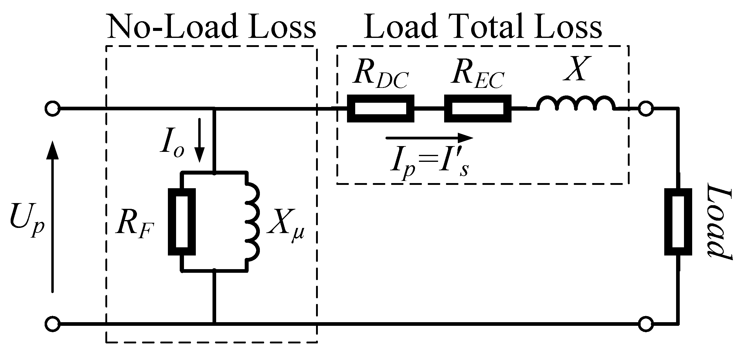
Figure 1 shows an approximated equivalent circuit corresponding to the power loss decomposition described in the standard [18] and formulated in (1). As mentioned above, the NLL can be found on the manufacturer datasheet or experimentally obtained from the open-circuit test. The TTL depends only on the load size and—according to the standard—is the sum of the three power loss components expressed in (2). When load current I reaches the nominal transformer current $I_n$, TLL is the short-circuit power $P_{K_n}$, i.e.,

$$\Delta P_{TTL}=P_{K_n}=I_n^2{R}_K$$

(7)

Therefore, the total loss resistance $R_{TTL}$ is the short circuit resistance $R_K$ which can be derived from the short-circuit power $P_{K_n}$ as follows

$$\Delta R_{TLL}=R_K={\displaystyle \frac{P_{K_n}}{I_n^2}}$$

(8)

From (2), (7), and (8) it is inferred that the TLL resistance in each phase is the sum of all resistances associated with the power load loss components, i.e.,

$$\Delta R_{TLL}=R_K=R_{DC}+R_{EC}+R_{OSL}$$

(9)

where $R_{DC}$ is the winding DC resistance, $R_{EC}$ is the winding EC resistance, and $R_{OSL}$ is the OSL resistance of the transformer. In contrast to what was stated in [33], the above resistance is dependent on the frequency. As will be discussed later in this paper, in the presence of higher current harmonics, $R_{TLL}$ inevitably increases due to the frequency dependence of $R_{EC}$ and $R_{OSL}$.

From (2) and (9), an equivalent expression is obtained:

$$\Delta P_{TLL}=I^2{R}_K=I^2\left(R_{DC}+R_{EC}+R_{OSL}\right)$$

(10)

Generally, the primary (p) and secondary (s) windings of a three-phase step-down distribution transformer are connected in a D/y configuration. As the primary windings of the transformer are delta-connected, current triplen harmonics do not appear at the transformer power supply network, i.e., the transformer primary side. However, they flow through and heat the primary windings—and hence their impact on TLL and its components must be considered. Each of the TLL components in (2) and (10) are calculated while considering the transformer winding connection.

3.1. DC Loss

The transformer DC loss per phase in (3) can be represented as the sum of primary and secondary winding DC loss:

$$\Delta P_{DC}=R_{D{C}_p}\sum _{\nu =1}^{\infty }{I}_{p_{\nu }}^2+R_{D{C}_s}\sum _{\nu =1}^{\infty }{I}_{s_{\nu }}^2$$

(11)

where $I_{p_{\nu }}$ and $I_{s_{\nu }}$ are the $\nu$-th current harmonics of, respectively, primary and secondary transformer sides. However, as the triplen harmonics cannot be measured at the primary side of a D/y connected transformer, (11) is modified as follows:

$$\Delta P_{DC}=R_{D{C}_p}\left(\sum _{\nu \ne 3,9,15,...}^{\infty }{I}_{p_{\nu }}^2+{\displaystyle \frac{1}{k^2}}\sum _{\nu =3,9,15,...}^{\infty }{I}_{s_{\nu }}^2\right)+R_{D{C}_s}\sum _{\nu =1}^{\infty }{I}_{s_{\nu }}^2$$

(12)

where both the primary and secondary DC resistances $R_{D{C}_p}$ and $R_{D{C}_s}$ can be directly measured or obtained from the manufacturer datasheet, and k is the transformer ratio between the primary and secondary phase voltages, $U_{p{h}_p}$ and $U_{p{h}_s}$, namely,

$$k={\displaystyle \frac{U_{p{h}_p}}{U_{p{h}_s}}}$$

(13)

Finally, the total DC resistance is derived by

$$R_{DC}=R_{D{C}_p}+k^2{R}_{D{C}_s}$$

(14)

3.2. WECL

Similarly to the DC resistance, $R_{EC}$ can be split into primary and secondary resistances, $R_{E{C}_p}$ and $R_{E{C}_s}$:

$$R_{EC}=R_{E{C}_p}+k^2{R}_{E{C}_s}$$

(15)

Since the ratio between primary and secondary DC resistances equals the ratio between primary and secondary EC resistances, i.e.,

$${\displaystyle \frac{R_{E{C}_p}}{R_{E{C}_s}}}={\displaystyle \frac{R_{D{C}_p}}{R_{D{C}_s}}}$$

(16)

$R_{E{C}_p}$ and $R_{E{C}_s}$ can be derived by solving Equations (15) and (16). Hence, in an analogous manner to the DC loss, eddy current loss can be represented as the sum of primary and secondary WECL and (4) becomes

$$\Delta P_{EC}=R_{E{C}_p}\sum _{\nu =1}^{\infty }{I}_{p_{\nu }}^2{\nu }^2+R_{E{C}_s}\sum _{\nu =1}^{\infty }{I}_{s_{\nu }}^2{\nu }^2$$

(17)

To account for the triplen harmonics effect, (17) is modified as follows:

$$\Delta P_{EC}=R_{E{C}_p}\left(\sum _{\nu \ne 3,9,15,...}^{\infty }{I}_{p_{\nu }}^2{\nu }^2+{\displaystyle \frac{1}{k^2}}\sum _{\nu =3,9,15,...}^{\infty }{I}_{s_{\nu }}^2{\nu }^2\right)+R_{E{C}_s}\sum _{\nu =1}^{\infty }{I}_{s_{\nu }}^2{\nu }^2$$

(18)

As mentioned above, the winding EC resistance depends on the frequency. This is represented by the ${\nu }^2$ factor in the above equation.

3.3. OSL

The OSL is independent of the transformer windings and can be associated with either side of the transformer. For a D/y connected distribution transformer, it is beneficial to correspond the OSL to the secondary where the triplen harmonics can be directly measured and modify (5) to become

$$\Delta P_{OSL}=R_{OSL}\sum _{\nu =1}^{\infty }{I}_{s_{\nu }}{\nu }^{0.8}$$

(19)

Hence, the OSL resistance referring to the secondary transformer side can be evaluated using (9) as follows:

$$R_{OSL}=R_K-R_{DC}-R_{EC}$$

(20)

As inferred from (19), $R_{OSL}$ is dependent on the harmonic frequency through a ${\nu }^{0.8}$ factor.

The nominal values of the WECL and OSL, as well as their associated resistances, are usually unspecified in the transformer technical documentation. Overcoming this can be achieved by employing the following relation:

$$R_{TSL}=R_{EC}+R_{OSL}$$

(21)

From (9) and (21), TSL resistance can be derived as follows:

$$R_{TSL}=R_K-R_{DC}$$

(22)

Since in oil-type transformers $\Delta P_{EC}=\Delta P_{OSL}$ [18], the following relation holds:

$$R_{EC}=R_{OSL}$$

(23)

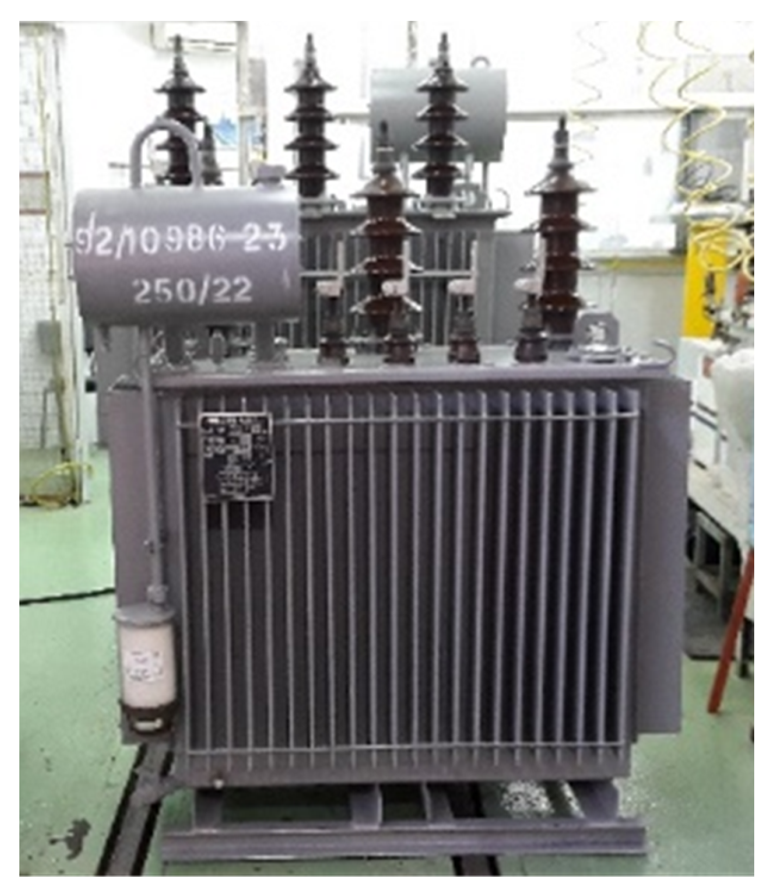
4. Experimental Setup

The method presented in this paper was experimentally validated through an experimental setup consisting of a full-scale 250 kVA D/y connected step-down 22/0.4 kV distribution oil-type transformer as shown in Figure 2. The transformer technical data is given in

Table 1. Transformer technical data.

Nominal apparent power	S	250 kVA
Connection	N/A	D/y
Nominal primary phase voltage	$U_{p{h}_{p}n}$	22 kV
Nominal secondary phase voltage	$U_{p{h}_{s}n}$	0.23 kV
Nominal primary phase current	$I_{p{h}_{p}n}$	3.79 A
Nominal secondary phase current	$I_{p{h}_{p}n}$	360.84 A
Frequency	f	50 Hz
Transformer ratio	k	95.65
Primary DC resistance	$R_{D{C}_p}$	40.5 $\Omega$
Secondary DC resistance	$R_{D{C}_s}$	0.0025 $\Omega$
No-load power	$P_0$	208 W
Short-circuit phase voltage	$U_{K_n}$	959 V
Short-circuit power	$P_{K_n}$	3257 V

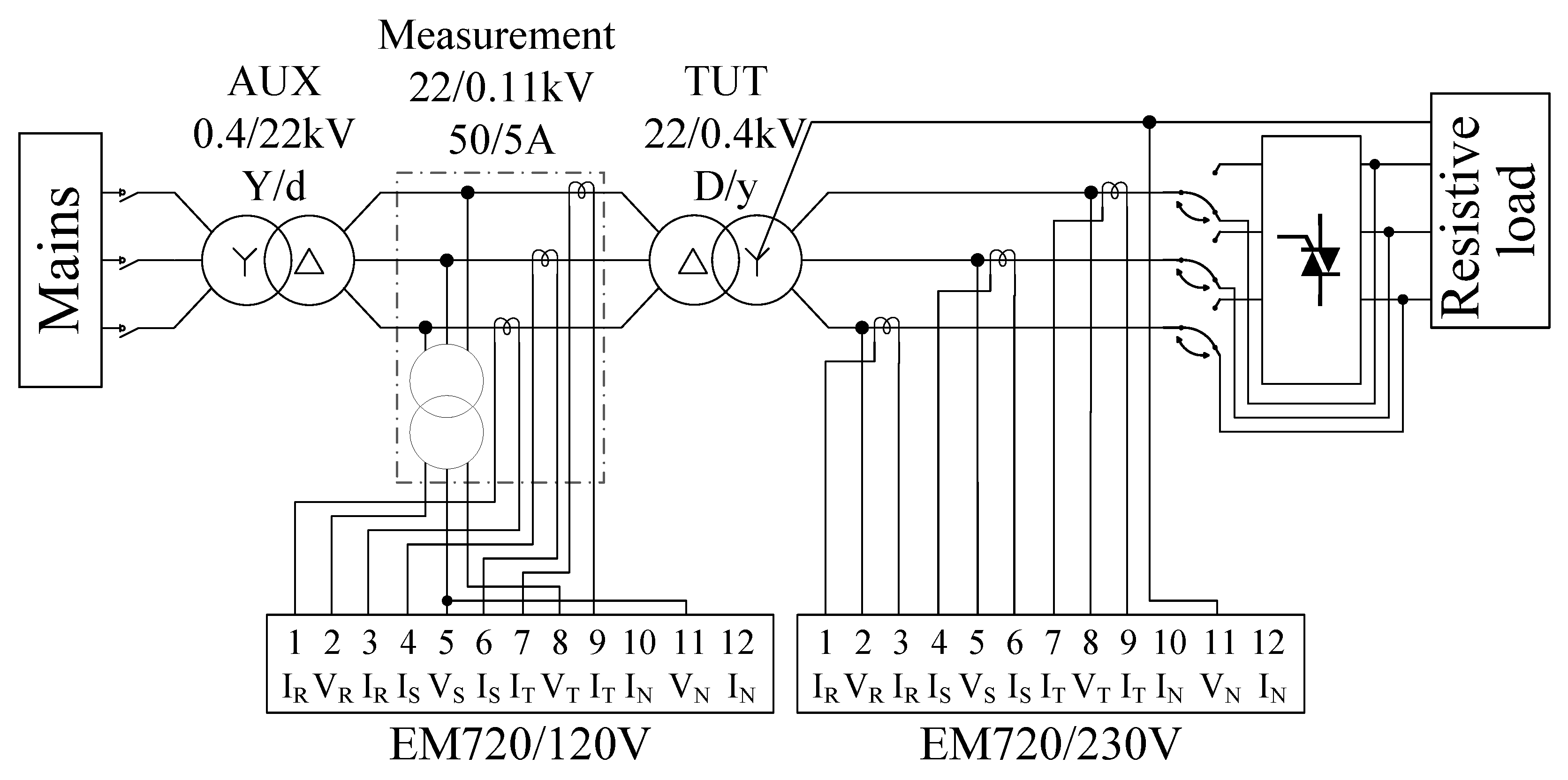
alongside its no-load and short-circuit test results while the experimental setup schematic is shown in Figure 3. For measurement purposes and mitigating the influence of adjacent electrical systems, the transformer under test (TUT) was connected to the electrical network through a 0.4 kV/22 kV Y/d auxiliary transformer (AUX).

Measurement of primary voltages, currents, and active power was performed using a SATEC 720 power analyzer Class 0.2S per IEC62053 [37] connected through a measurement tank—comprising a three-phase voltage transformer 22/0.11 kV and three single-phase current transformers 50/5 A. The accuracy of the measuring voltage transformer is 0.2%, and the accuracy of the measuring current transformers is 0.25%. An additional SATEC 720 was connected at the low-voltage side to measure secondary voltages, currents, and active power. The voltages were measured directly while obtaining the secondary currents in each phase, and the power analyzer was connected via three current transformers, 400/5 A of class 0.2.

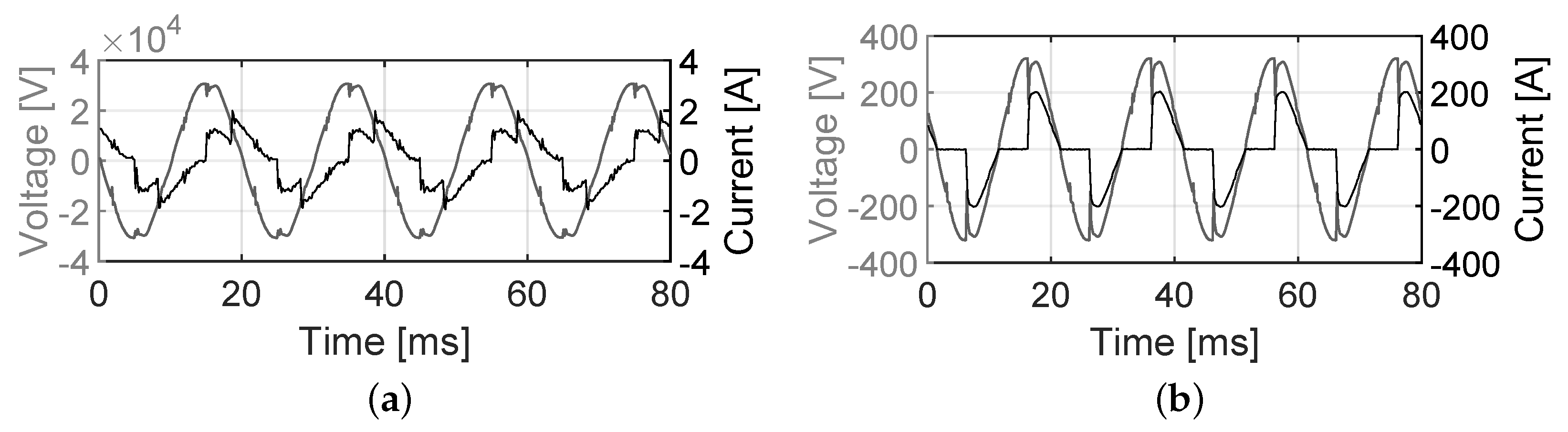
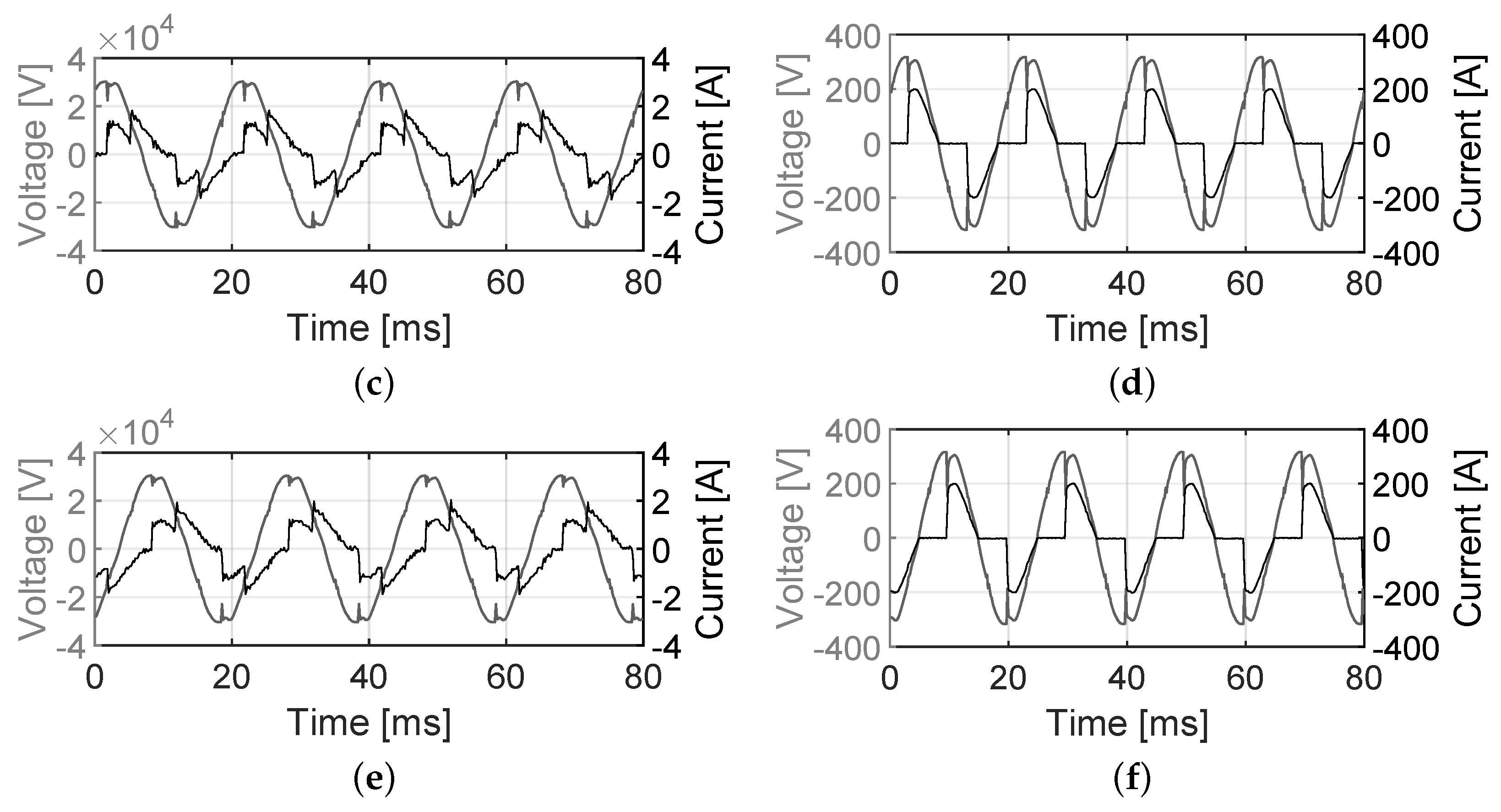
As depicted in Figure 3, the secondary side of the TUT was connected to a pair of resistive load+TPC and a thyristor power controller (TPC) [38] which utilized a three-phase nonlinear load. Due to the limitations of laboratory circuit-breakers, the TUT was not fully loaded.

The fundamental active power $P_1$ and power components corresponding with the $\nu$-th harmonic $P_{\nu }$ flow in opposite directions [39]. The active powers $P_P$ and $P_S$ are measured, respectively, at the primary and secondary transformer sides. Hence, the TTL was obtained as follows:

$$\Delta P_{TTL}=P_p-P_s$$

(24)

where

$$\Delta P_p=P_{p_1}-\sum _{\nu =2}^{\infty }{P}_{p_{\nu }}$$

(25)

and

$$\Delta P_s=P_{s_1}-\sum _{\nu =2}^{\infty }{P}_{s_{\nu }}$$

(26)

where $P_{p_1}$ and $P_{p_{\nu }}$ are, respectively, the fundamental and $\nu$-th active power components measured at the primary side. Similarly, $P_{s_1}$ and $P_{s_{\nu }}$ are, respectively, the fundamental and $\nu$-th active power components measured at the secondary side.

By substituting (25) and (26) into (24), the following is obtained:

$$\Delta P_{TTL}=\left(P_{p_1}-P_{s_1}\right)+\sum _{\nu =1}^{\infty }\left(P_{s_{\nu }}-\Delta P_{p_{\nu }}\right)=\Delta P_1+\Delta P_{\nu }$$

(27)

where

$$\Delta P_1=\left(P_{p_1}-P_{s_1}\right)$$

(28)

and

$$P_{\nu }=\sum _{\nu =1}^{\infty }\left(P_{s_{\nu }}-\Delta P_{p_{\nu }}\right)$$

(29)

are, respectively, the transformer loss components due to the fundamental and $\nu$-th current harmonics.

5. Experimental Results

5.1. Calculation of TLL Resistance Components

Using (8), the equivalent resistance $R_K$ referring to the primary side is calculated to be 75.57 $\Omega$. Based on the DC resistances of each winding, the total DC resistance component as expressed by (14) is 63.37 $\Omega$. The TSL resistance $R_{TSL}$, obtained using (22), is 12.20 $\Omega$. Substituting in (21) and employing (23), the total WECL and the OSL resistances, referring to the primary side, are both 6.10 $\Omega$.

Four experimental operating points were obtained by setting the firing angle $\alpha$ of the TPC to 0°, 45°, 90°, and 135°. For each angle, voltage and current harmonics, the phase between them, and the harmonic active power components were measured at each side of the transformer.

Calculation of power components using the proposed approach is given here in detail for firing angle 45° while the experimental results and data for the remaining three firing angles are provided in the Appendix A. Figure 4 shows experimental results for the primary and secondary voltages and currents. The measured data for firing angle 45° is given in

Table 2. Primary measurement data for firing angle $\alpha =45°$.

$\mathit{\nu }$	${\mathit{U}}_{\mathit{p},\mathit{\nu }}$[V]			${\mathit{I}}_{\mathit{p},\mathit{\nu }}$[A]			${\mathit{\phi }}_{\mathit{p},\mathit{\nu }}$[°]			${\mathit{P}}_{\mathit{p},\mathit{\nu }}$[W]
	R	S	T	R	S	T	R	S	T	R	S	T
1	21,563	21,470	21,506	1.41	1.40	1.40	14.1	14	13.9	29,417	29,251	29,312
3	50.13	25.23	35.48	0	0	0	N/A	N/A	N/A	0	0	0
5	121.3	93.93	155.38	0.179	0.183	0.184	−30.70	−25.37	−25.37	18.66	15.55	25.84
7	489.49	462.15	473.12	0.112	0.124	0.107	−10.82	−11.38	−11.18	53.81	56.09	49.71
9	39.89	43.47	10.75	0	0	0	N/A	N/A	N/A	0	0	0
11	217.25	203.43	204.84	0.043	0.050	0.044	−19.58	−19.95	−20.16	8.72	9.65	8.43
13	248.52	213.09	197.31	0.050	0.057	0.046	16.13	15.62	15.56	12.04	11.71	8.70
15	38.81	37.57	5.91	0	0	0	N/A	N/A	N/A	0	0	0

and

Table 3. Secondary measurement data for firing angle $\alpha =45°$.

$\mathit{\nu }$	${\mathit{U}}_{\mathit{s},\mathit{\nu }}$[V]			${\mathit{I}}_{\mathit{s},\mathit{\nu }}$[A]			${\mathit{\phi }}_{\mathit{s},\mathit{\nu }}$[°]			${\mathit{P}}_{\mathit{s},\mathit{\nu }}$[W]
	R	S	T	R	S	T	R	S	T	R	S	T
1	224.5	224.9	224.8	133.0	131.90	132.30	10.85	10.70	10.75	29,345	29,148	29,225
3	3.72	3.7	3.48	25.44	24.87	24.97	−32.94	−32.54	−34.92	79.44	77.57	71.24
5	2.58	2.33	2.04	17.83	17.98	17.91	−24.64	−21.74	−24.88	41.76	38.96	33.15
7	7.43	7.54	7.41	10.88	10.58	10.84	−11.75	−11.98	−11.88	79.16	78.00	78.69
9	2.53	2.54	2.69	6.07	6.05	6.08	−11.11	−10.50	−10.59	15.08	15.13	16.09
11	3.42	3.50	3.34	4.71	4.65	4.62	21.22	20.73	21.47	15	15.24	14.37
13	3.87	3.66	3.59	4.58	4.54	4.63	−9.57	−9.78	−9.37	17.45	16.38	16.42
15	2.97	3.13	3.06	4.48	4.35	4.32	−6.44	−6.59	−6.43	13.23	13.53	13.15

for, respectively, the primary and secondary sides. The measured and calculated values for harmonics of an order higher than 15 were found to be negligible and were omitted.

The total fundamental active three-phase power at the secondary transformer side is 87,718.88 W, while the measured total power due to voltage and current harmonics is 759.03 W. From (26), the total active power on the secondary side is 86,959.85 W. Similarly, the total fundamental active power and the measured total power due to voltage and current harmonics at the primary side are, respectively, 87,980.67 W and 278.89 W. From (25), the total active power on the primary side is 87,701.79 W.

The TTL was directly calculated from the power measurements using (24) to be 741.93 W.

5.2. Proposed Method Results

The NLL was experimentally obtained from the open-circuit test at nominal input voltage and found to be 208 W. As mentioned above, the TLL was calculated by employing (12), (18), and (19).

5.2.1. DC Loss Calculation

Both the primary and secondary DC resistances $R_{D{C}_p}$ and $R_{D{C}_s}$ were measured directly to be, respectively, 40.5 $\Omega$ and 0.0025 $\Omega$. From (12), the calculated DC loss is 395.4 W.

5.2.2. WECL Calculation

The WECL was found using (18) to be 101.4 W, while—by employing (15) and (16)—the EC resistances $R_{E{C}_p}$ and $R_{E{C}_s}$ were found to be, respectively, 3.89 $\Omega$ and 0.00024 $\Omega$.

5.2.3. OSL Calculation

An OSL of 42.92 W was calculated using (19) with a total OSL resistance—as referred to the secondary transformer side—of 0.00067 $\Omega$.

From (1) and (2), the total calculated loss is 747.69 W, which matches closely with the measured TTL of 741.93 W, featuring an error margin smaller than 0.8.

5.3. Measured vs. Calculated Results

Table 4. Calculated vs. measured data for firing angles 0, $\alpha =45°$, $\alpha =90°$, and $\alpha =135°$.

		Calculated						Measured
$\mathit{\alpha }°$	$\Delta {\mathit{P}}_{\mathit{NL}}$[W]	$\Delta {\mathit{P}}_{\mathit{DC}}$[W]	$\Delta {\mathit{P}}_{\mathit{EC}}$[W]	$\Delta {\mathit{P}}_{\mathit{OSL}}$[W]	$\Delta {\mathit{P}}_{\mathit{TTL}}$[W]	${\mathit{THD}}_{\mathit{i},\mathit{P}}$[%]	${\mathit{THD}}_{\mathit{i},\mathit{S}}$[%]	$\Delta {\mathit{P}}_{\mathit{TTL}}$[W]	$\mathit{ϵ}$[%]
0	208	439.16	43.38	42.48	733.02	0	0	747.58	1.95
45	208	395.37	101.4	42.92	747.69	16.1	25.7	741.93	0.78
90	208	225.2	131.4	32.26	596.86	24.7	60.4	579.94	2.92
135	208	45.4	66.58	9.69	329.67	65.1	112.8	320.4	2.89

summarizes the calculated loss components for the four firing angles used in this study. All experimental results show good compatibility with the theoretical model, featuring a maximum error margin of less than 3%.

6. Conclusions

This paper presented an application of a transformer loss calculation method under nonlinear loads to a full-scale 250 kVA D/y connected step-down 22/0.4 kV distribution oil-immersed transformer which is widely used in distribution networks. Application of the method to oil-type transformers is salient as it extends the method’s validity from a non-standard bare dry-type laboratory transformer to a widely used standard distribution liquid-immersed transformer. This is particularly important in light of the loss characteristic variability between these two types of transformers—as appears in both research papers and the standard.

In contrast to other methods published in the literature, the proposed method relies solely on readily available data and can serve as an alternative to the approach detailed in IEEE std. C57.110-2018. The proposed method also considers the heating effect due to triplen harmonics in a delta-connected transformer winding—a phenomenon which is not addressed by the standard. Finally, the proposed method evaluates per-phase power loss and hence can be applied for imbalanced loading scenarios.

A series of experiments for one linear and three nonlinear loading scenarios were performed and showed a close match to the theoretical model with a maximum error margin smaller than 3%. This outcome is substantially lower than the 5–7.5% error levels reported in the literature as detailed in the Section 1.

Future work shall explore the application of the proposed method for developing a techno-economic model for optimal transformer asset management in power grids.

References

1. Stoyanov, T.; Spasov, R.; Rizov, P. Power transformers supplied by non-sinusoidal voltages or supplying non-linear loads- problems and solutions. In Proceedings of the 2022 14th Electrical Engineering Faculty Conference (BulEF), Varna, Bulgaria, 14–17 September 2022; pp. 1–4. [Google Scholar] [CrossRef]
2. Xu, X.; Collin, A.; Djokic, S.; Yanchenko, S.; Moeller, F.; Meyer, J.; Langella, R.; Testa, A. Analysis and Modelling of Power-Dependent Harmonic Characteristics of Modern PE Devices in LV Networks. IEEE Trans. Power Delivery 2017, 32, 1014–1023. [Google Scholar] [CrossRef]
3. Slonim, M.; Braunstein, A.; Miteva, N. The harmonic contents of electronic device currents: Experimental, qualitative and theoretical analysis. In Proceedings of the IEEE PowerTech Budapest 99, Budapest, Hungary, 29 August–2 September 1999; Volume 229. [Google Scholar] [CrossRef]
4. Chakravorty, D.; Meyer, J.; Schegner, P.; Yanchenko, S.; Schocke, M. Impact of Modern Electronic Equipment on the Assessment of Network Harmonic Impedance. IEEE Trans. Smart Grid 2017, 8, 382–390. [Google Scholar] [CrossRef]
5. Deokar, S.; Waghmare, L. Analysis of Distribution Transformer Performance under Non-linear Balanced Load Conditions and its Remedial Measures. Int. J. Emerg. Technol. Adv. Eng. 2011, 1, 152–161. [Google Scholar]
6. Bureau of Energy Efficiency. Best Practice Manual–Transformers; Indian Renewable Energy Development Agency, Devki Energy Consultancy Pvt. Ltd.: Gujarat, India, 2006. [Google Scholar]
7. EN 50160-2010; Voltage Characteristics of Electricity Supplied by Public Electricity Networks. CENELEC—European Committee for Electro technical Standardization: Brussels, Belgium, 2010.
8. IEEE Std 519-2014; IEEE Recommended Practice and Requirements for Harmonic Control in Electric Power Systems (Revision of IEEE Std 519-1992). IEEE: Piscataway, NJ, USA, 2014; pp. 1–29. [CrossRef]
9. Amin, U.; Talib, A.; Qureshi, S.A.; Hossain, M.J.; Ahmad, G. Comparison of Electrical Parameters of Oil-Immersed and Dry-Type Transformer Using Finite Element Method. Int. J. Energy Power Eng. 2018, 12, 337–341. [Google Scholar]
10. Dawood, K.; Gezer, F.; Köse, F.; Tursun, S. Experimental Assessment of No-Load and Load Losses in Dry-Type and Oil-Filled Transformers. In Proceedings of the 2024 16th Electrical Engineering Faculty Conference (BulEF), Varna, Bulgaria, 19–22 September 2024; pp. 1–4. [Google Scholar] [CrossRef]
11. Thungsuk, N.; Mungkung, N.; Tanaram, T.; Chaithanakulwat, A.; Arunrungsusmi, S.; Poonthong, W.; Songruk, A.; Tunlasakun, K.; Chunkul, C.; Tanitteerapan, T.; et al. The Characterization Analysis of the Oil-Immersed Transformers Obtained by Area Elimination Method Design. Appl. Sci. 2022, 12, 3970. [Google Scholar] [CrossRef]
12. Olivares, J.C.; Liu, Y.; Canedo, J.M.; Escarela-Perez, R.; Driesen, J.; Moreno, P. Reducing losses in distribution transformers. IEEE Trans. Power Deliv. 2003, 18, 821–826. [Google Scholar] [CrossRef]
13. Godina, R.; Rodrigues, E.M.G.; Matias, J.C.O.; Catalão, J.P.S. Effect of Loads and Other Key Factors on Oil-Transformer Ageing: Sustainability Benefits and Challenges. Energies 2015, 8, 12147. [Google Scholar] [CrossRef]
14. Thakur, S.; Butlero, N.M.; Holbøll, J. Effects of harmonics on temperature rise and power loss of a distribution transformer. In Proceedings of the 2022 9th International Conference on Condition Monitoring and Diagnosis (CMD), Kitakyushu, Japan, 13–18 November 2022; pp. 732–735. [Google Scholar] [CrossRef]
15. Tandeaw, P.; Manop, C.; Jirasuwankul, N. Design and Testing of Low Loss Distribution Transformer for Non-Linear Loading Current. In Proceedings of the 2018 International Electrical Engineering Congress (iEECON), Krabi, Thailand, 7–9 March 2018; pp. 1–4. [Google Scholar] [CrossRef]
16. Thango, B.A.; Akuru, U.B.; Nnachi, A.F. Corrected Estimation of the Transformer Winding Eddy Losses for Utility-Scale Solar Photovoltaic Plant Application. In Proceedings of the 2021 International Conference on Electrical, Computer and Energy Technologies (ICECET), Cape Town, South Africa, 9–10 December 2021; pp. 1–5. [Google Scholar] [CrossRef]
17. Alawasa, K.M.; Al-Badi, A.H. Investigation and Analysis of the Power Quality in an Academic Institution’s Electrical Distribution System. Energies 2024, 17, 3998. [Google Scholar] [CrossRef]
18. IEEE Std C57.110™-2018; IEEE Recommended Practice for Establishing Liquid-Immersed and Dry-Type Power and Distribution Transformer Capability When Supplying Nonsinusoidal Load Currents (Revision of IEEE Std C57.110-2008). IEEE: Piscataway, NJ, USA, 2018; pp. 1–68. [CrossRef]
19. Seddik, M.S.; Eteiba, M.B.; Shazly, J. Evaluating the Harmonic Effects on the Thermal Performance of a Power Transformer. Energies 2024, 17, 4871. [Google Scholar] [CrossRef]
20. Gouda, O.E.; Amer, G.M.; Salem, W.A.A. Predicting transformer temperature rise and loss of life. Ain Shams Eng. J. 2012, 3, 113–121. [Google Scholar] [CrossRef]
21. Mitra, B.; Singhal, A.; Kundu, S.; Ogle, J.P. Analyzing Distribution Transformer Degradation with Increased Power Electronic Loads. In Proceedings of the 2023 IEEE Power & Energy Society Innovative Smart Grid Technologies Conference (ISGT), Washington, DC, USA, 16–19 January 2023; pp. 1–5. [Google Scholar] [CrossRef]
22. Kelley, A.W.; Edwards, S.W.; Rhode, J.P.; Baran, M.E. Transformer derating for harmonic currents: A wide-band measurement approach for energized transformers. IEEE Trans. Ind. Appl. 1999, 35, 1450–1457. [Google Scholar] [CrossRef]
23. Taher, M.A.; Kamel, S.; Ali, Z.M. K-Factor and transformer losses calculations under harmonics. In Proceedings of the 2016 Eighteenth International Middle East Power Systems Conference (MEPCON), Cairo, Egypt, 27–29 December 2016; pp. 753–758. [Google Scholar] [CrossRef]
24. Yildirim, D.; Fuchs, E.F. Measured transformer derating and comparison with harmonic loss factor (F/sub-HL/) approach. IEEE Trans. Power Deliv. 2000, 5, 186–191. [Google Scholar] [CrossRef]
25. Hesterman, B. Time-Domain K-Factor Computation Methods. In Proceedings of the PCIM’94, Official Proceedings of the Twenty-Ninth International Power Conversion Conference, Dallas, TX, USA, 17–22 September 1994. [Google Scholar]
26. Ruiz, I.R.M.; Guajardo, L.A.T.; Alfaro, L.H.R.; Salinas, F.S.; Maldonado, J.R.; Vázquez, M.A.G. Design Implication of a Distribution Transformer in Solar Power Plants Based on Its Harmonic Profile. Energies 2021, 14, 1362. [Google Scholar] [CrossRef]
27. Thango, B.A.; Bokoro, P.N. Defining and Specifying Design Considerations for Distribution Transformers in Large-Scale Solar Photovoltaic Plants. Energies 2022, 15, 2773. [Google Scholar] [CrossRef]
28. Ma, X.; Jia, R.; Liang, C.; Du, H.; Dong, X.; Ding, M. Study of Transformer Harmonic Loss Characteristic in Distribution Network Based on Field-Circuit Coupling Method. Sustainability 2022, 14, 12975. [Google Scholar] [CrossRef]
29. Sima, L.; Miteva, N.; Dagan, K.J. A Novel Approach to Power Loss Calculation for Power Transformers Supplying Nonlinear Loads. Electr. Power Syst. Res. 2023, 223, 109582. [Google Scholar] [CrossRef]
30. Yanchenko, S.; Meyer, J. Harmonic emission of household devices in presence of typical voltage distortions. In Proceedings of the 2015 IEEE Eindhoven PowerTech, Eindhoven, The Netherlands, 29 June–2 July 2015; pp. 1–6. [Google Scholar] [CrossRef]
31. Wan, D.; You, K.; Zhou, H.; Qi, F.; Peng, S.; Peng, T. Study on Harmonic Load Loss Calculation Method of Oil-Paper Insulated Distribution Power Transmission Equipment. In Proceedings of the 2019 IEEE 3rd Conference on Energy Internet and Energy System Integration (EI2), Changsha, China, 8–10 November 2019; pp. 2746–2749. [Google Scholar] [CrossRef]
32. Abdulveleev, I.R.; Khramshina, E.A.; Druzhinin, N.N.; Gasiyarov, V.R. Impact of Service Life Duration on Electric Losses in Power Transformers: An Analytical Review. In Proceedings of the 2023 International Ural Conference on Electrical Power Engineering (UralCon), Magnitogorsk, Russia, 29 September–1 October 2023; pp. 801–806. [Google Scholar] [CrossRef]
33. Plienis, M.; Deveikis, T.; Jonaitis, A.; Gudžius, S.; Konstantinavičiūtė, I.; Putnaite, D. Improved Methodology for Power Transformer Loss Evaluation: Algorithm Refinement and Resonance Risk Analysis. Energies 2023, 16, 7837. [Google Scholar] [CrossRef]
34. Fuchs, E.F.; Yildirim, D.; Grady, W.M. Measurement of eddy-current loss coefficient P/sub-EC-R/, derating of single-phase transformers, and comparison with K-factor approach. IEEE Trans. Power Deliv. 2000, 15, 148–154. [Google Scholar] [CrossRef]
35. Li, P.; Li, G.; Xu, Y.; Yao, S. Methods Comparation and Simulation of Transformer Harmonic Losses. In Proceedings of the 2010 Asia-Pacific Power and Energy Engineering Conference, Chengdu, China, 28–31 March 2010; pp. 1–4. [Google Scholar] [CrossRef]
36. Shepelev, A.O.; Petrova, E.V.; Sidorov, O.A. Consideration of Active Resistances Temperature Dependency of Power Transformers when Calculating Power Losses in Grids. In Proceedings of the 2018 International Conference on Industrial Engineering, Applications and Manufacturing (ICIEAM), Moscow, Russia, 15–18 May 2018; pp. 1–5. [Google Scholar] [CrossRef]
37. SATEC. Power Quality and Revenue Meter EM720/EM720T. Available online: https://www.satec-global.com/wp-content/uploads/2022/12/EM720-Installation-Manual.pdf (accessed on 16 June 2025).
38. Solcon. Thyristor Power Controller: TPS. Available online: https://www.aef-hitachi.cz/files/download/softstartery-brzdy/rvs-dxm-1/tps-silver.pdf/ (accessed on 16 June 2025).
39. Lipsky, A.M.; Miteva, N.V.; Lokshin, E.S. Current harmonics and commercial losses in smart grids. In Proceedings of the 2012 3rd IEEE PES Innovative Smart Grid Technologies Europe (ISGT Europe), Berlin, Germany, 14–17 October 2012; pp. 1–5. [Google Scholar] [CrossRef]
Figure 1. Equivalent single-line transformer schematic.
Electronics 14 02500 g001
Figure 2. The 250 kVA distribution oil-type transformer under test.
Electronics 14 02500 g002
Figure 3. Experimental setup schematic.
Electronics 14 02500 g003
Figure 4. Voltage (gray) and current (black) waveforms for firing angle α = 45°; primary side: (a) phase R, (b) phase S, and (c) phase T; secondary side: (d) phase R, (e) phase S, and (f) phase T.
Electronics 14 02500 g004