Article

A Convex Constraint Approach for High-Type Control Loop Design

1
Key Laboratory of Optical Engineering, Chinese Academy of Sciences, Chengdu 610209, China
2
National Key Laboratory of Optical Field Manipulation Science and Technology, Chinese Academy of Sciences, Chengdu 610209, China
3
Institute of Optics and Electronics, Chinese Academy of Sciences, Chengdu 610209, China
4
University of Chinese Academy of Sciences, Beijing 100049, China
5
Independent Researcher, Nanjing 211135, China
*
Author to whom correspondence should be addressed.
Electronics 2025, 14(12), 2491; https://doi.org/10.3390/electronics14122491
Submission received: 17 April 2025 / Revised: 15 June 2025 / Accepted: 16 June 2025 / Published: 19 June 2025

Abstract

This paper proposes a high-type control loop design method for LQR-LMI based on Lyapunov and polyhedral model theory. The high-type control loop design problem is simplified into a convex constraint problem, which achieves superior tracking performance. In this framework, the input amplitude of the control signal, the poles of the closed-loop system, the suppression of external interference and the perturbation of internal parameters are considered, and the linear matrix inequality (LMI) method is effectively used to solve the problems. In this paper, the polyhedral model control theory is introduced to characterize the uncertainty of the system for the change of model parameters of the controlled plant. Aiming at the problem of external disturbance suppression, the H 2 / H control method is introduced into the system. These control methods provide the basis for the design of the high-type control loop. Compared with the simulation results of other optimization algorithms, the effectiveness and superiority of the controller parameter tuning rules in the proposed high-type control loop are verified.

1. Introduction

The electro-optical tracking system is widely used in fields such as astronomical observation, aerospace and quantum communication [1,2]. Most early electro-optical tracking systems were ground-based acquisition, tracking and pointing (ATP) systems, such as large telescopes and electro-optical theodolites. With the expansion of application fields, electro-optical tracking systems have gradually been installed on moving platforms such as automobiles, ships, aircraft and satellites to meet different mission requirements. Different from ground-based electro-tracking equipment, the electro-optical tracking system based on moving platforms faces greater technical challenges in line-of-sight (LOS) stabilization. Vehicle motion-induced vibrations and jitter impose severe external disturbances on the system, while internal perturbations such as parameter uncertainties compound the issue. These combined disturbances cause LOS jitter, leading to blurred target imagery and image instability on TV detectors. Such effects degrade the accuracy of miss distance extraction and undermine the system’s overall tracking stability precision [3,4]. Therefore, it is critical to develop methods that enable the system to rapidly and precisely suppress both internal and external disturbances while achieving target tracking.
The Proportional–Integral–Derivative (PID) closed-loop controller in traditional electro-optical tracking systems remains one of the most favored and widely adopted control strategies [5,6]. However, with the complexification of application environments, the model uncertainty of the controlled object has become increasingly non-negligible. The traditional linear predictive PID control method, designed based on a fixed linearized model around the operating point, can no longer meet the control performance requirements. Additionally, this method lacks strong corrective capabilities for compensating nonlinearities, time delays and disturbances [7]. Against this backdrop, researchers have explored polyhedral model control theory to address nonlinear and uncertain systems, providing a new perspective for the analysis and design of control systems. The polyhedral model control theory utilizes convex combination modeling to characterize uncertainties in the controlled plant as a linear combination of a finite set of vertex models [8,9]. This framework offers a rigorous theoretical basis and efficient problem-solving strategies for tackling the challenges of model mismatch and system uncertainties discussed earlier. Currently, the emergence of linear matrix inequality (LMI) technology has provided a powerful tool for the development of polyhedral model control theory [10,11,12]. By combining polyhedral models with LMIs, complex control problems can be transformed into convex optimization problems, enabling their solution using existing optimization algorithms. This gives polyhedral model control theory significant advantages in handling nonlinear systems, model uncertainties, and constraint conditions, allowing for the effective design of controllers that meet performance requirements. In recent years, research on polyhedral model control theory lies in expanding application boundaries (such as time-delay, nonlinear, and distributed systems) and cross-theoretical integration (with event triggering, neural networks, fuzzy control, etc.). Through these efforts, polyhedral model theory is moving from traditional academic research to practical engineering scenarios such as aerospace, intelligent transportation, and industrial automation, and has become one of the key tools for solving the control of complex and uncertain systems.
With the development of control theory, optimal control theories such as linear quadratic regulator (LQR), sliding mode control and high-type control have provided new approaches for addressing control problems in uncertain complex systems [13,14,15]. It is worth noting that linear optimal controllers among these methods are predominantly designed using the LQR approach. This approach can effectively handle system uncertainties and external disturbances, designing optimal control strategies based on system states and objective functions to achieve precise control of the plant [16,17]. However, when dealing with multi-constraint problems, the traditional LQR method relies on an accurate system model and has limited capability to handle multiple constraints. Especially when the constraints are in the form of nonlinearities or inequalities, they are difficult to integrate directly into the optimization framework. This may cause the solution to deviate from practical requirements or fail to satisfy the constraints. Additionally, the closed-loop gain matrix of LQR is obtained by solving the algebraic Riccati equation, a process that exhibits high computational complexity in high-dimensional systems and is sensitive to model parameter perturbations, resulting in insufficient robustness [18]. The high-type control enhances the system’s type by adding integral links, thereby improving the system’s tracking ability and disturbance rejection ability [19,20]. Currently, the vast majority of research on high-type control focuses on the frequency-domain design of the system, ignoring the requirements in the time-domain. Although the high-type control method can strengthen the system’s tracking and disturbance rejection capabilities, the tuning of its controller parameters has always been challenging in both the academic and engineering fields.
To address the limitations of the LQR method and high-type control mentioned above, LMI technology can effectively compensate for their shortcomings. LMI technology boasts powerful multi-constraint expression capabilities, enabling the transformation of various linear or nonlinear constraints—such as state amplitude limits, input saturation constraints, and robust stability conditions—into matrix inequality forms, which can then be solved through a unified convex optimization framework [21,22]. Additionally, LMI technology can be efficiently solved via mature convex optimization algorithms and supports parallel computing, making it suitable for high-dimensional systems and large-scale optimization problems. This provides a more universal solution for the optimal control of multi-constraint systems.
In general, single optimization control struggles to comprehensively and efficiently meet complex and changeable control requirements in practical applications. It is necessary to organically integrate and coordinate multiple control strategies to effectively address complex control problems. This paper proposes an LQR-LMI high-type control loop design method based on Lyapunov theory and polyhedral model theory to tackle the problem of the system tracking fast signals under multiple constraints. The main contributions of this paper are as follows:
(i)
This paper proposes a high-type control loop design method for LQR-LMI based on Lyapunov and polyhedral model theory. The high-type control loop design problem is simplified into a convex constraint problem, which achieves higher tracking accuracy and stronger disturbance suppression ability.
(ii)
In this paper, the input amplitude of the control signal, disturbance suppression and other practical requirements are considered in the design of high-type control loops, which are expressed as LQR cost, H 2 / H performance, regional pole constraint and so on. Then the LMI method is used to effectively solve the problem.
(iii)
Compared with the simulation results of other optimization algorithms (ITAE, ITSE, ISE, IAE), the effectiveness and superiority of the controller parameter tuning rules in the proposed high-type control loop are verified.
The rest of the paper is organized as follows. In Section 2, the design theory of the LQR-LMI high-type control loop based on Lyapunov and polyhedral model theory is given. Section 3 conducts simulation analysis and experimental verification. Finally, the summary is given in Section 4.

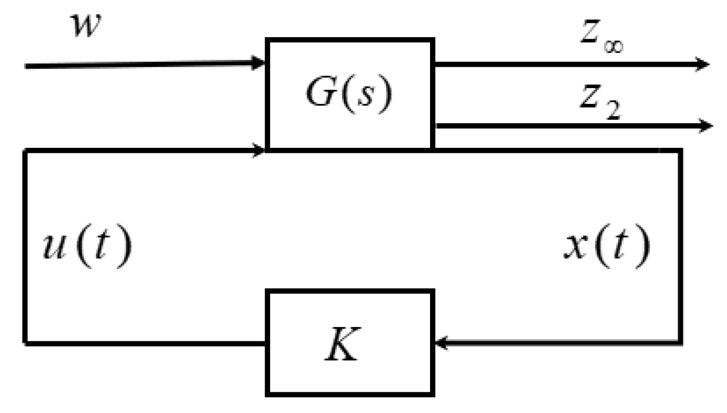
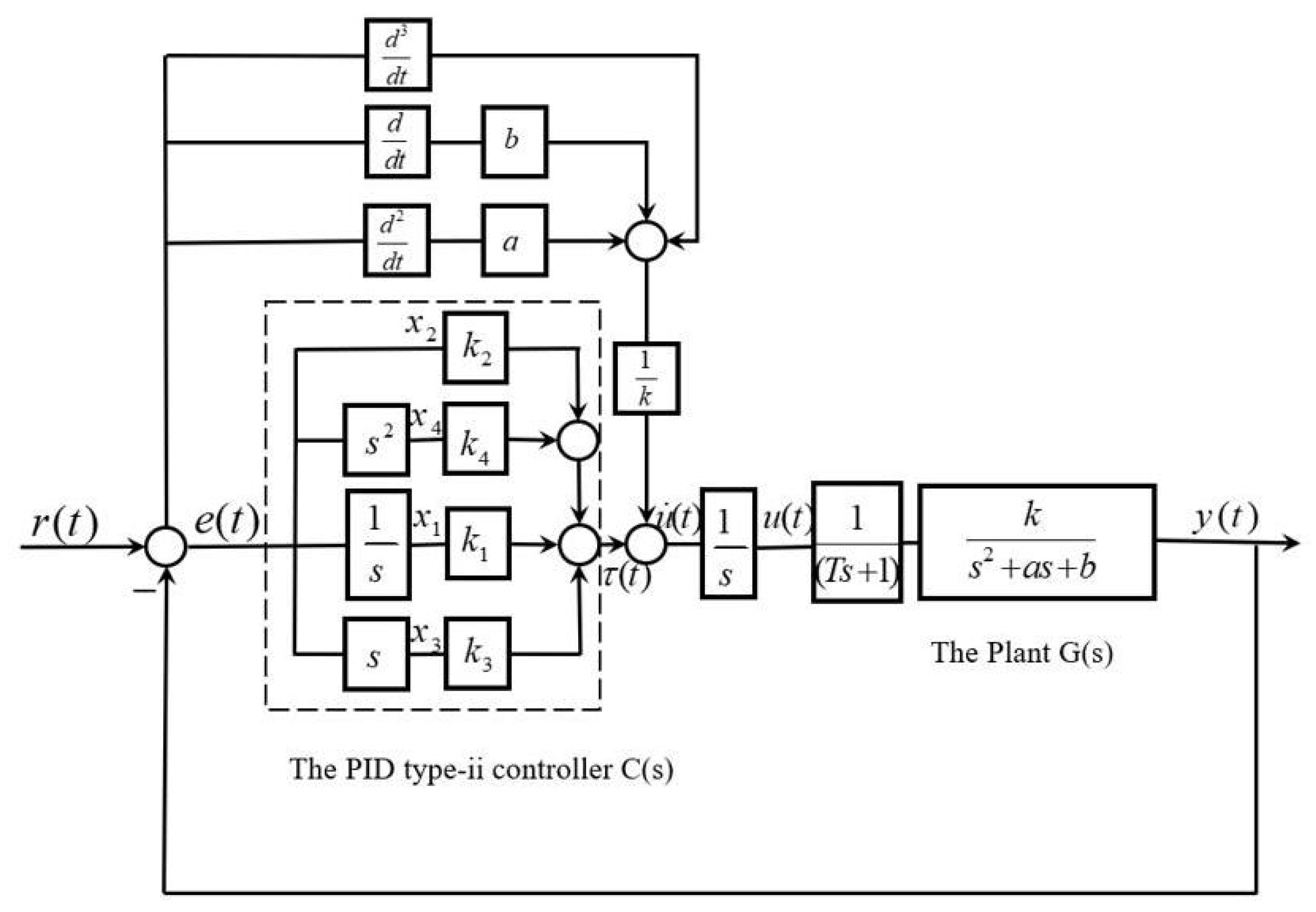
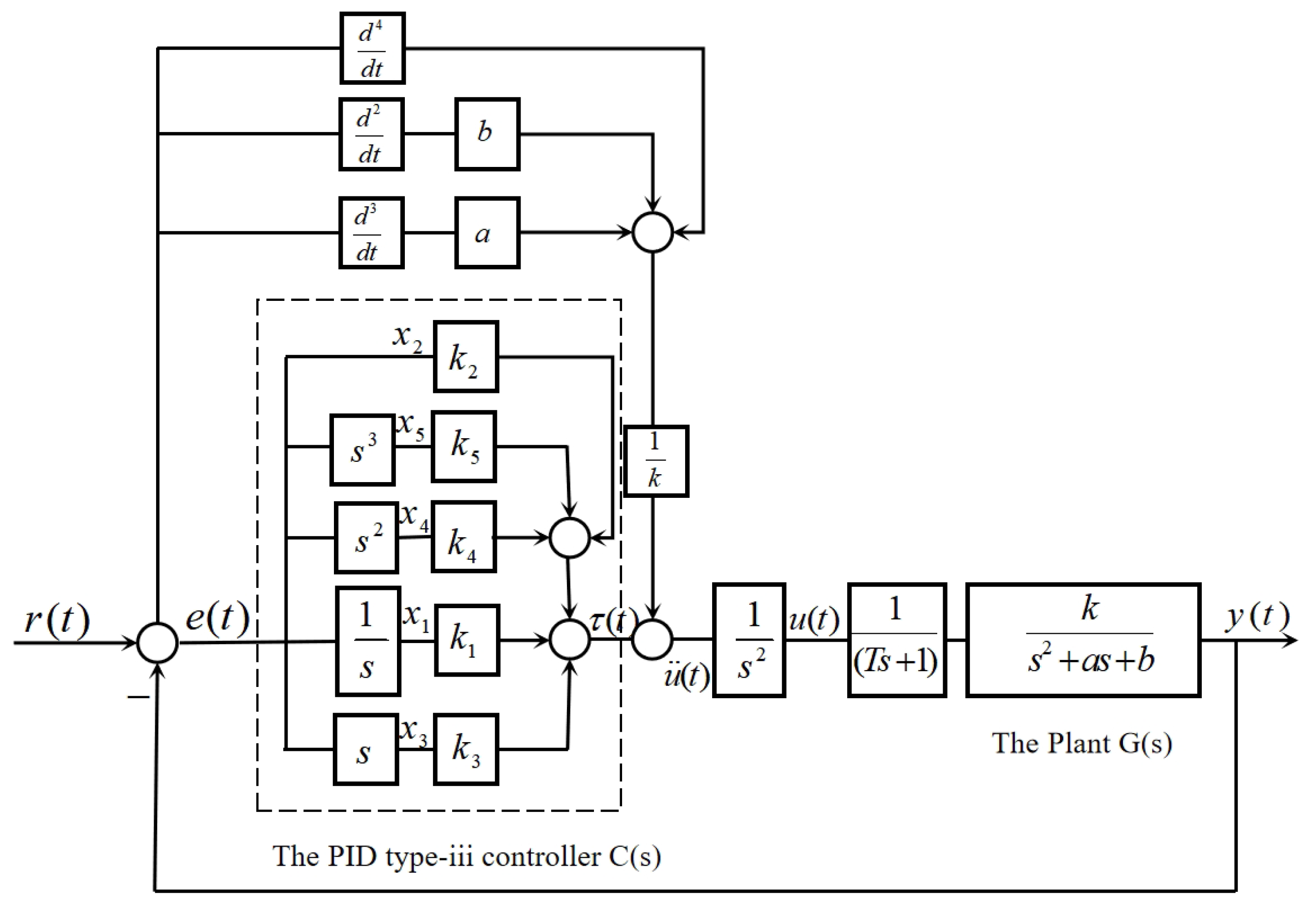
2. The Theory of Controller Parameter Tuning in the High-Type Control Loop

Consider a time-invariant linear system
x o ˙ ( t ) = A o x o ( t ) + B o u ( t ) u ( t ) = K x o ( t ) ,
where A o , B o , x o ( t ) , u ( t ) , K are the state transition matrix, control matrix, state matrix, control input and controller parameters, respectively.
For the linear system in Equation (1), to achieve exponential convergence of the Lyapunov function, the following linear inequality constraint should be guaranteed [23]:
λ P 1 ^ + A o P 1 ^ + B o Y 1 + P 1 ^ A o T + P 1 ^ Y 1 T < 0 ,
where λ > 0 , P 1 ^ = P 1 , P > 0 , P = P T .
Proof. 
According to the Lyapunov stability, the following Lyapunov function V is chosen:
V = x o T Px o .
The convergence effect of x o can be effectively adjusted by adjusting the design of P .
Substituting Equation (1) into the derivative of Lyapunov function V , we get
V ˙ = x o ˙ T Px o + x o T P x o ˙ = A o x o + B o u T Px o + x o T P A o x o + B o u = x o T A o + B o K T Px o + x o T P A o + B o K x o = x o T Q 1 T x o + x o T Q 1 x o = x o T ε x o ,
where Q 1 = P ( A o + B o K ) , ε = Q 1 T + Q 1 .
To achieve x o exponential convergence, i.e., V ˙ λ V , take
λ V + V ˙ = λ x o T Px o + x o T ε x o = x o T λ P + ε x o .
If we take λ P + ε < 0 and λ > 0 , then V ˙ λ V . From V ˙ λ V , we can get
V ( t ) V ( 0 ) e λ t V ( 0 ) ,
where V ( 0 ) = x 0 T P x 0 ϖ . If t , then V ( t ) 0 , i.e., x o 0 and it converges exponentially.
We expand out λ P + ε < 0 ; we get
λ P + PA + PBK + A T P + K T B T P < 0 .
Since Equation (7) contains nonlinear terms, it must be transformed into the LMI to be solved. We multiply the left and right ends of Equation (7) by P 1 and we get the Equation (2). The proof process is complete. □

The LQR-LMI Framework

The initial value of the system state in Equation (1) is 0, and the corresponding quadratic performance index is defined as
J = 0 x o T ( t ) Q o x o ( t ) + u T ( t ) R o u ( t ) d t ,
where Q o and R o are symmetric positive semidefinite matrix and symmetric positive definite matrix, respectively. According to the LQR control theory, the control input is
u ( t ) = K x o ( t ) = R o 1 B o T P x o ( t ) ,
where P is the solution of the following nonlinear equation.
A o T P + P A o + Q o P B o R o 1 B o T P = 0 .
And, the minimum quadratic form performance index of Equation (1) is
J min = x o T ( 0 ) P x o ( 0 ) .
The LQR method has limited capability to handle multiple constraints, and its solution relies on solving the algebraic Riccati equation in Equation (5). Therefore, the LQR problem in Equation (6) by the LMI technique can be rephrased as an optimization problem over P 1 ^ and Y 1 :
J min P 1 ^ , Y 1 = x o T ( 0 ) P 1 ^ x o ( 0 ) ϖ
subject to
A o P 1 ^ + P 1 ^ A o T + B o Y 1 + Y 1 T B o T P 1 ^ Y 1 T P 1 ^ Q o 1 0 Y 1 0 R o 1 0 , P 1 ^ > 0 ,
where ϖ is the specified upper bound, Y 1 = K P 1 ^ , P 1 ^ = P 1 . According to Schur complement theorem, the above Equation (7) can be expressed as
ϖ x o T ( 0 ) x o ( 0 ) P 1 ^ 0 .
Firstly, the problem that the system matrix [ A o , B o ] is not accurate in practice is considered. In general, the polyhedral model control theory is adopted to characterize the uncertainties of the system. Through convex combination modeling, the uncertainties of the controlled plant in Equation (1) are described as a linear combination of a finite number of vertex models, namely [ A o , B o ] belongs to a polyhedral set [24]:
Ω 1 = C o w A 1 , B 1 , A 2 , B 2 , , A H m , B H m
where C o w refers to a convex hull, or A o , B o Ω 1 if
[ A o , B o ] = i = 1 H m g i ( x , u ) A i , B i ,
where H m is the number of multiple models and g i the weighting functions constrained between 0 and 1, and this satisfies
i = 1 H m g i ( x , u ) = 1 , ( x , u ) R n x × R n u .
Secondly, the H 2 / H control method in Figure 1 is adopted to consider the problem of system interference suppression [25]. The aim is to design a controller such that the closed-loop system is asymptotically stable, namely G p ( s ) < γ p and G o ( s ) 2 < γ o , where
G p ( s ) = C p + D p 1 K sI A o + B o K 1 B w + D p 2
and
G o ( s ) = C o + D o 1 K sI A o + B o K 1 B w .
Suppose the polyhedral model of interference [26] w is
x o ˙ = A o x o + B o u + B w w z p = C p x + D p 1 u + D p 2 w z o = C o x + D o 1 u ,
where z o and z p are the output vectors; w is the disturbance vector; A o , B o , B w , C , C o , D p 1 , D p 2 , and D o 1 are matrices of system coefficients.
Substituting the controller feedback gain Equation (4) into Equation (15), the corresponding closed-loop system is
x o ˙ = A o + B o K x o + B w w z p = C p + D p 1 K x o + D p 2 w z o = C o + D o 1 K x o .
Assuming that
P ^ = P ^ 2 = Δ P ^ 1 ,
Y = Y 2 = Δ Y 1 ,
according to the following theorem to solve the optimal symmetric positive definite matrix P ^ 1 and matrix Y 1 .
Lemma 1.
For the polyhedral model in Equation (15) with interference and a given scalar γ p > 0 , there exists an optimal solution (symmetric positive definite matrices P 1 ^ and Y 1 ) satisfying the following LMI [23]:
A i P 1 ^ + B i Y 1 T + A i P 1 ^ + B i Y 1 B w C p P 1 ^ + D p 1 Y 1 T B w T γ p I D p 2 T C p P 1 ^ + D p 1 Y 1 D p 2 γ p I < 0 A i P 1 ^ + B i Y 1 + A i P 1 ^ + B i Y 1 T + B w B w T < 0 Z C o P 1 ^ + D o 1 Y 1 C o P 1 ^ + D o 1 Y 1 T P 1 ^ < 0 trace ( Z ) < γ o 2 i = 1 , 2 H m .
Next, the closed-loop pole of the system is constrained to the left of the complex s-plane to achieve the stability of the system. In addition, to achieve good transient performance, an integral term is added so that the steady-state error of the system output is zero. The closed-loop poles of the system are constrained between α and β on the left side of the complex s-plane if and only if there exist matrices P 1 ^ and Y 1 satisfying [23]:
2 α P 1 ^ + A o P 1 ^ + B o Y 1 + Y 1 T B o T + P 1 ^ T A o T < 0 2 β P 1 ^ + A o P 1 ^ + B o Y 1 + Y 1 T B o T + P 1 ^ T A o T > 0 .
Finally, the input amplitude of the control signal is considered. The inequality constraints governing the physical limits of the input amplitudes of the signals are designed according to the following Lemma 2.
Lemma 2
([27]). For the control signal u u max , where u max is the maximum input amplitude of the control signal, the relevant linear inequality matrix must satisfy the following relation:
k 0 P 1 ^ P 1 ^ K T K P 1 ^ 1 0 ,
where k 0 = ϖ 1 u max 2 .
Ultimately, the controller feedback gain is calculated using the following algorithm:
Step 1: Determine the parameters of A i , B i , C p , D p 1 , D p 2 , C o and D o 1 .
Step 2: Select appropriate λ , upper bound value ( ϖ ) of LQR performance index, maximum input amplitude of controller u ( t ) , specified scalar γ p , the pole of closed-loop system α , the pole of closed-loop system β , the initial state x o ( 0 ) and weighting matrix Q o > 0 , R o > 0 .
Step 3: By solving Equations (2), (13), (14) and (24)–(26), solve the optimal solution P 1 ^ and Y 1 .
Step 4: The controller feedback gain in the related control loop is solved by Equation (27).
K = Y 1 P 1 ^ 1 .
The uncertain plant in the type-ii control loop is
G 11 ( s ) = y ( s ) u ( s ) = k s ( s 2 + a s + b ) ,
where a = 2 ζ o ω o l , b = ω o l 2 , where ζ o , ω o l are the damping ratio and natural frequency of the open-loop plant, respectively. k is the system open-loop gain. The system parameters vary in intervals:
a a ̲ , a ¯ , b b ̲ , b ¯ , k k ̲ , k ¯ ,
where a ̲ and a ¯ , b ̲ and b ¯ , k ̲ and k ¯ denote the lower and upper bounds of the corresponding parameter interval, respectively.
The correlation weighting matrix is set as Q o = d i a g q 1 , q 2 , q 3 , q 4 and R o = r 1 , where q 1 , q 2 , q 3 , q 4 , r 1 are the weighting coefficients, respectively. In Figure 2, τ ( t ) can be expressed as
τ ( t ) = Kx o = k 1 x 1 ( t ) + k 2 x 2 ( t ) + k 3 x 3 ( t ) + k 4 x 4 ( t ) ,
where
x 1 ( t ) = e ( t ) d t , x 2 ( t ) = e ( t ) , x 3 ( t ) = d e ( t ) / d t , x 4 ( t ) = d 2 e ( t ) / d t ,
k 1 , k 2 , k 3 , k 4 are the coefficients before the corresponding states of the system, respectively.
The state-space equation of the uncertain plant in Equation (28) is modeled as
x ˙ 1 ( t ) x ˙ 2 ( t ) x ˙ 3 ( t ) x ˙ 4 ( t ) = 0 1 0 0 0 0 1 0 0 0 0 1 0 0 b a x 1 ( t ) x 2 ( t ) x 3 ( t ) x 4 ( t ) + 0 0 0 k τ ( t ) ,
where τ ( t ) = u ˙ ( t ) r + a r ¨ + b r ˙ k .
The uncertain plant in the type-iii control loop is
G 22 ( s ) = y ( s ) u ¨ ( s ) = k s 2 s 2 + a s + b .
The correlation weighting matrix is set as Q o = d i a g q 1 , q 2 , q 3 , q 4 , q 5 and R o = r 1 , where q 1 , q 2 , q 3 , q 4 , q 5 , r 1 are the weighting coefficients, respectively. In Figure 3, τ ( t ) can be expressed as
τ ( t ) = k 1 x 1 ( t ) + k 2 x 2 ( t ) + k 3 x 3 ( t ) + k 4 x 4 ( t ) + k 5 x 5 ( t ) ,
where
x 1 ( t ) = e ( t ) d t , x 2 ( t ) = e ( t ) , x 3 ( t ) = d e ( t ) / d t , x 4 ( t ) = d 2 e ( t ) / d t , x 5 ( t ) = d 3 e ( t ) / d t .
The state-space equation of the uncertain plant in Equation (33) is modeled as
x ˙ 1 ( t ) x ˙ 2 ( t ) x ˙ 3 ( t ) x ˙ 4 ( t ) x ˙ 5 ( t ) = 0 1 0 0 0 0 0 1 0 0 0 0 0 1 0 0 0 0 0 1 0 0 0 b a x 1 ( t ) x 2 ( t ) x 3 ( t ) x 4 ( t ) x 5 ( t ) + 0 0 0 0 k τ ( t ) ,
where τ ( t ) = u ¨ ( t ) r + a r + b r ¨ k .

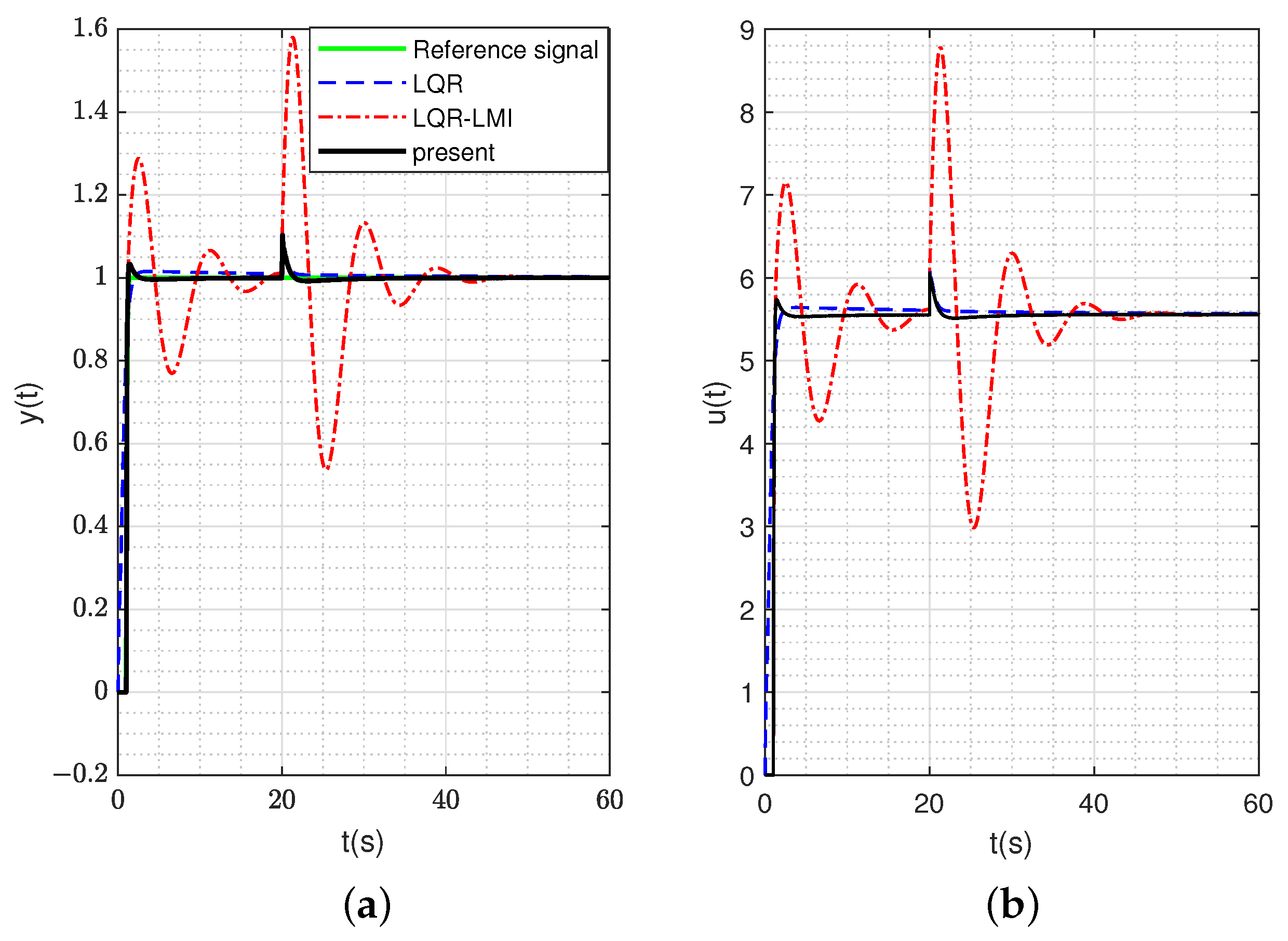
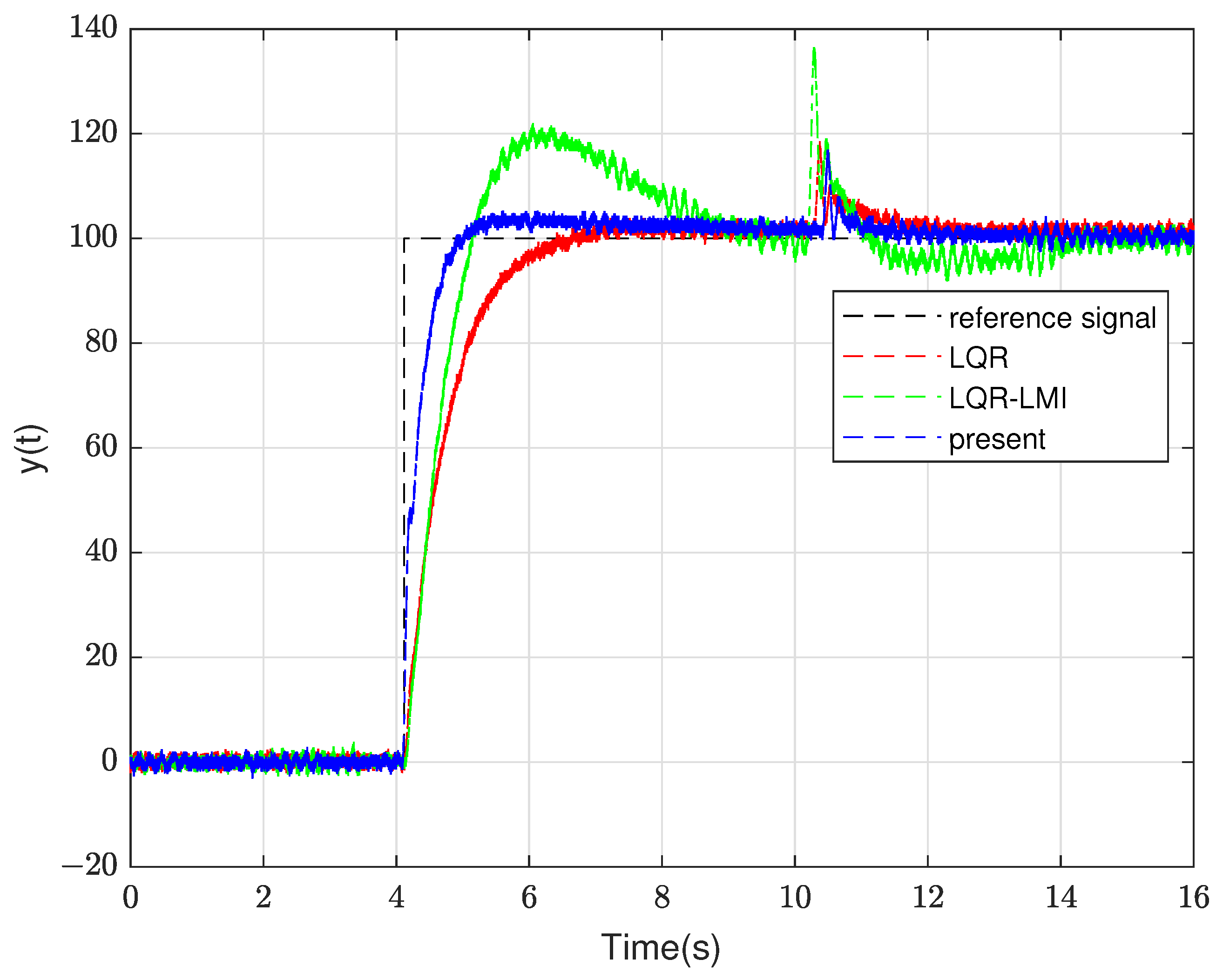
3. Simulation Analysis and Experimental Verification

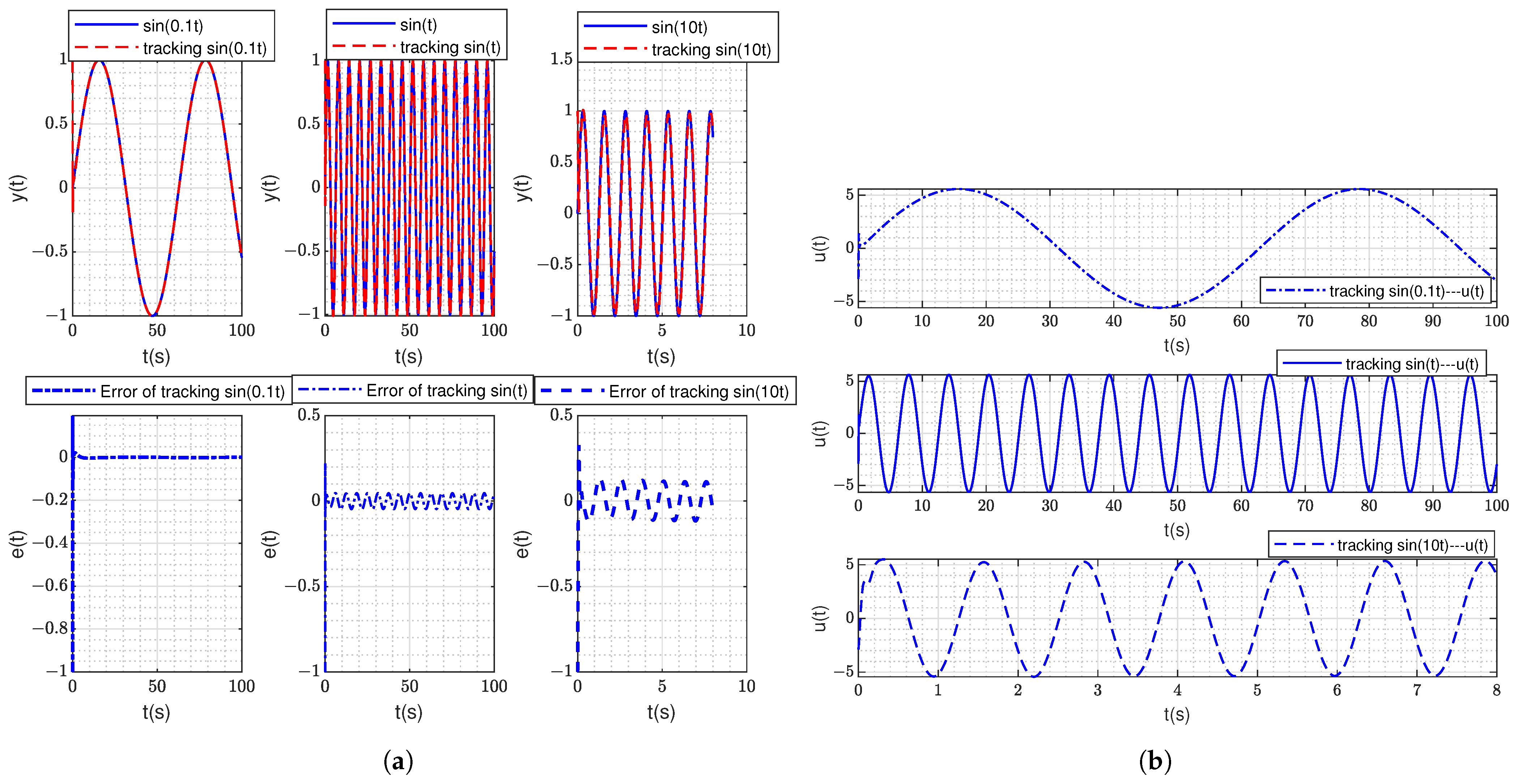
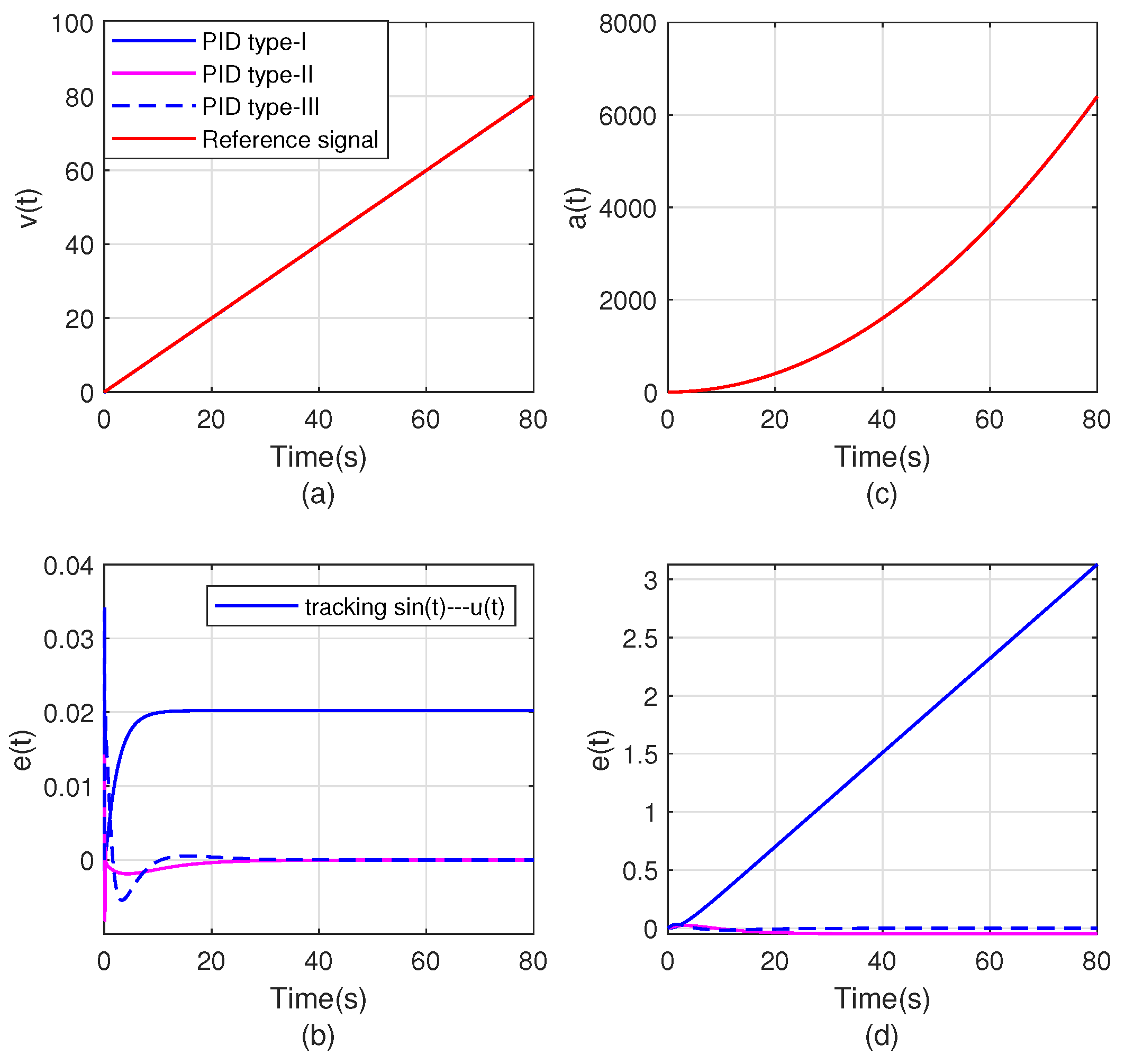
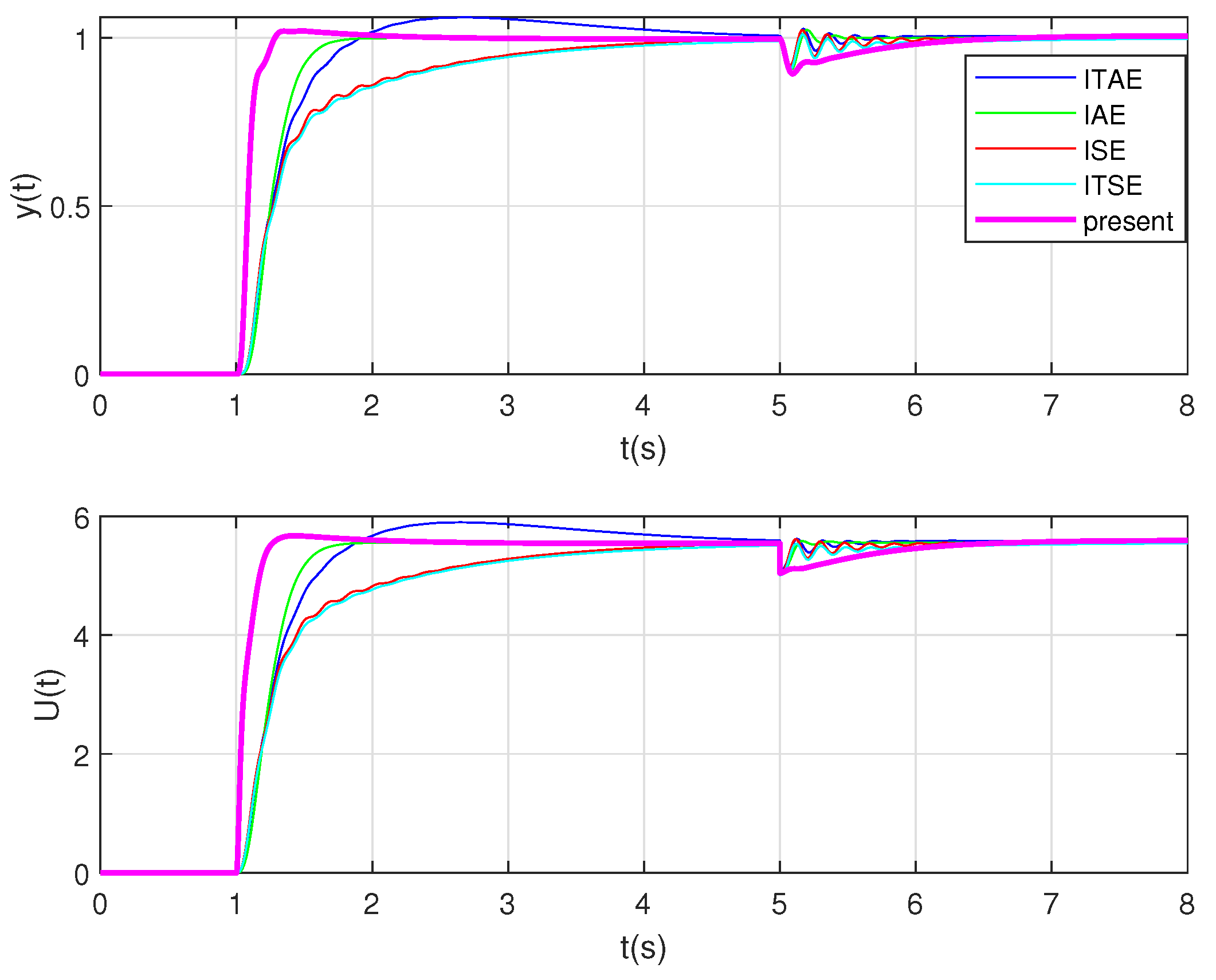
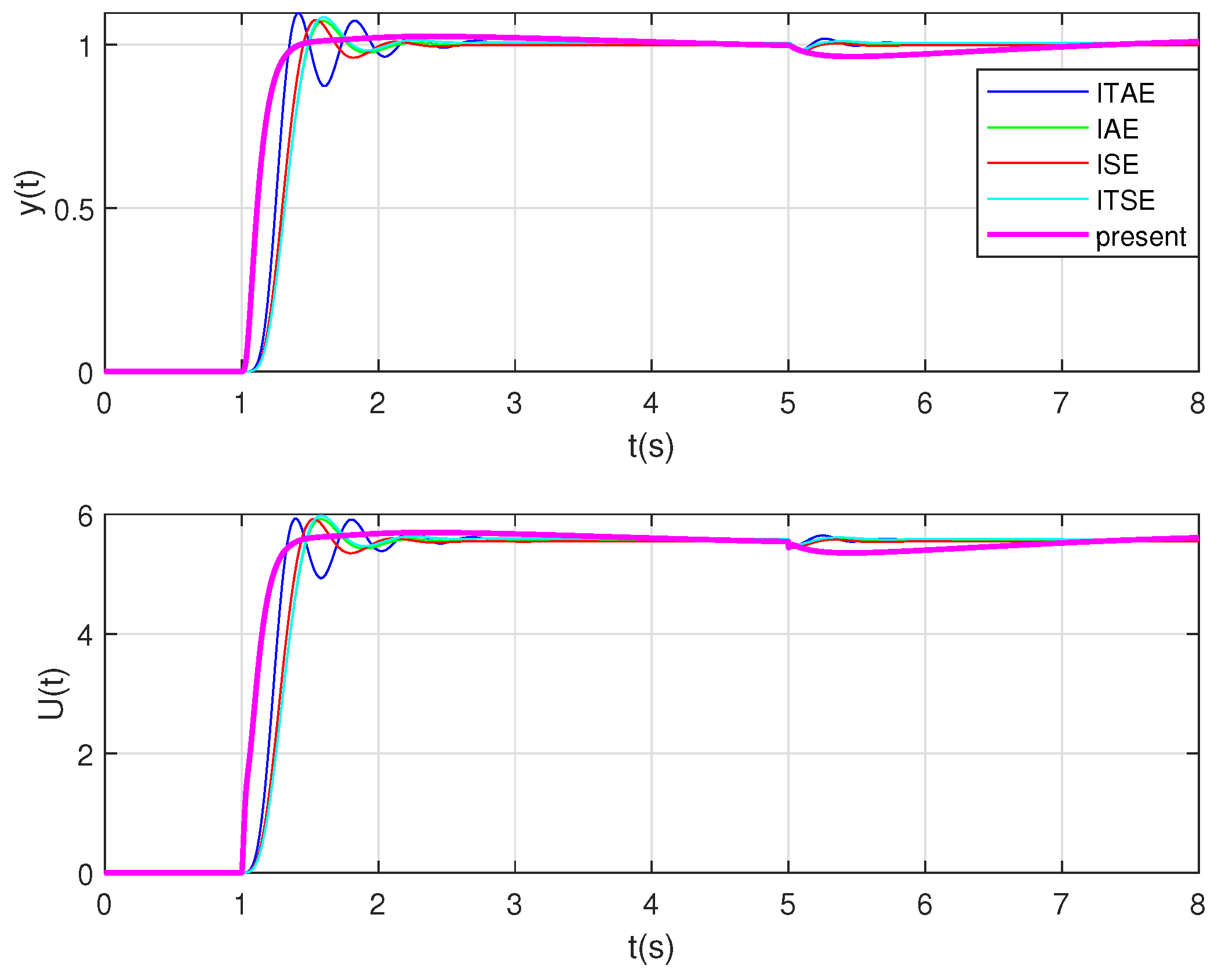
3.1. The Simulation Part of the High-Type Control Loop

The characteristics of the electro-optical tracking system in Equation (50) are represented by
G ( s ) = 1776.4 s 2 + 25.6 s + 1421.2 .
In this study, the natural frequency is mainly considered to change between 90 % and 110 % of the original frequency, that is, the system parameter interval changes as
a 23.2 , 28.4 , b 932.2 , 1393.1 , k 167.8 , 250.8 .
Therefore, the vertex matrix A i , B i i = 1 , 2 8 is
A 1 = A 2 = 0 1 0 0 0 1 0 932 . 2 23 . 2 , A 3 = A 4 = 0 1 0 0 0 1 0 1393 . 1 23 . 2 , A 5 = A 6 = 0 1 0 0 0 1 0 932 . 2 28 . 4 , A 7 = A 8 = 0 1 0 0 0 1 0 1393 . 1 28 . 4 , B 1 = B 3 = B 5 = B 7 = 0 0 167 . 8 , B 2 = B 4 = B 6 = B 8 = 0 0 250 . 8 .
In the type-ii control loop, λ is 0.1, the upper bound value ( ϖ ) of the LQR performance index is 5, the maximum input amplitude of controller u ( t ) is 10, the specified scalar γ p = 2000 , the system closed-loop pole α = 0.1 , the system closed-loop pole β = 100 and the weighting matrix Q o = d i a g 0.0001 , 1 , 0.0001 , 0.0001 and R o = 0.01 .
For disturbance w L 2 0 , + , the H / H 2 closed-loop system has disturbance suppression performance under the specified scalar γ p > 0 , i.e.,
0 q 1 x 1 2 ( t ) + q 2 x 2 2 ( t ) + q 3 x 3 2 ( t ) + q 4 x 4 2 ( t ) + r u 2 ( t ) d t < 0 w 2 ( t ) d t .
Assuming that
C p = C o = q 1 0 0 0 0 q 2 0 0 0 0 q 3 0 0 0 0 q 4 0 0 0 0 , D p 1 = D o 1 = 0 0 0 0 r , D p 2 = 0 , B w = 0 1 0 0 .
According to Equations (2), (13), (14) and (24)–(27), the controller under the proposed method is
C I I 1 ( s ) = 1.4428 + 8.257 s + 0.4187 s 2 + 0.0719 s 3 s 2 ( 0.1 s + 1 ) .
Similarly, the controller based on the LQR-LMI method is
C I I 2 ( s ) = 0.106 + 0.4043 s 5.1043 s 2 0.0728 s 3 s 2 ( 0.1 s + 1 ) .
To illustrate the effectiveness and superiority of the LMI method and the polyhedral model control method, the weighting matrix Q o and R o in the LQR method should be set to be consistent with the weighting matrix in the proposed method. The controller tuned by the LQR method is
C I I 3 ( s ) = 0.1 + 10.0584 s + 0.2976 s 2 + 0.0439 s 3 s 2 ( 0.1 s + 1 ) .
Figure 4a shows the step response of the system controlled by different methods under 50 % external disturbance at t = 20 s. By comparing the response curves under the LQR method and the LQR-LMI method in Figure 4a, the LQR-LMI method is superior to the LQR method. Compared with the LQR method, the LQR-LMI method has the advantage of introducing the LMI method in the LQR-LMI method. The LQR-LMI method can easily deal with the solution of constraint problems such as controller design specification in practical applications. Similarly, by comparing the response curves under the proposed method, the LQR method and the LQR-LMI method in Figure 4a, the proposed method is significantly better than the LQR-LMI method and the LQR method.
Figure 4b shows the response of the controller by different methods under 50 % external disturbance at t = 20 s. It can be seen that the response of the controller under the proposed method is better than that of the LQR-LMI method and the response of the controller under the LQR method. Meanwhile, the response of the controller under the method in this paper conforms to the maximum input amplitude of controller u ( t ) that we initially set as 10.
In the above PID type-ii control loop, the poles of the closed-loop system controlled by the proposed method are s 1 = 19.4089 + 27.7094 i , s 2 = 19.4089 27.7094 i , s 3 = 1.2366 , s 4 = 0.2049 . To illustrate the role of the polyhedral model theory, by changing the natural frequency of plants, the control effects of the method proposed in this paper and the LQR-LMI method were compared, as shown in Figure 5. In this study, the natural frequency variation interval of the plant, such as Equation (37), is set as 20.9 , 46.9 and varies within the range of 33.9 Hz.
By comparing Figure 5a,c, it can be seen that when the natural frequency of the plant is changed, that is, the natural frequency is changed in the range of 20.9 , 46.9 , the step response of the system under the proposed method in this paper is almost not affected by the change of the natural frequency of the plant. This also shows the effectiveness of the introduction of polyhedral model theory in the method of this paper. Meanwhile, the step response under the proposed method is significantly better than that under the LQR-LMI method, that is, the rise time and settling time under the proposed method are significantly improved. And the overshoot is small. By comparing Figure 5b,d, results consistent with those mentioned above can be obtained.
Figure 6 shows the tracking response of sinusoidal signals of different frequencies under the proposed method. The initial state of the system is set as x 0 = 0 1 1 0 .
Figure 6a shows the tracking response and tracking error of sin(0.1t), sin(t) and sin(10t) under the proposed method. In Figure 6a, the red curve represents the tracking of the reference signal using the proposed method. The sinusoidal instruction signals, such as sin(0.1t), sin(t) and sin(10t), can be effectively tracked by using the proposed method. Meanwhile, the error of the system tracking sin(0.1t), sin(t) and sin(10t) instruction signals is very small. Figure 6b shows the controller response of sin(0.1t), sin(t) and sin(10t) under the proposed method. The limit value of controller response meets u ( t ) < 5 and the maximum input amplitude of controller u ( t ) is in line with our initial setting of 10.
In the type-iii control loop, λ is 0.1, ( ϖ ) is 5, the maximum input amplitude of controller u ( t ) is 10, the specified scalar γ p = 2000 , the system closed-loop pole α = 0.1 , the system closed-loop pole β = 100 and the weighting matrix Q o = d i a g 0.0001 , 1 , 0.0001 , 0.0001 , 0.0001 and R o = 0.01 .
For disturbance w L 2 0 , + , the H / H 2 closed-loop system has disturbance suppression performance under the specified scalar γ p > 0 , i.e.,
0 q 1 x 1 2 ( t ) + q 2 x 2 2 ( t ) + q 3 x 3 2 ( t ) + q 4 x 4 2 ( t ) + q 5 x 5 2 ( t ) r u 2 ( t ) d t < 0 w 2 ( t ) d t .
Assuming that
C p = C o = q 1 0 0 0 0 0 q 2 0 0 0 0 0 q 3 0 0 0 0 0 q 4 0 0 0 0 0 q 5 0 0 0 0 0 , D p 1 = D o 1 = 0 0 0 0 0 r , D p 2 = 0 , B w = 0 1 0 0 0 .
According to Equations (2), (13), (14) and (24)–(27), the controller under the proposed method is
C I I I 1 ( s ) = 0.1289 + 1.4327 s + 4.9474 s 2 0.9029 s 3 + 0.2119 s 4 s 3 ( 0.1 s + 1 ) .
The controller based on the LQR-LMI method is
C I I I 2 ( s ) = 0.0453 + 0.2411 s + 0.3445 s 2 5.1617 s 3 0.0737 s 4 s 3 ( 0.1 s + 1 ) .
Similarly, to illustrate the effectiveness and superiority of the LMI method and the polytopic model control method introduced in this paper in the type-iii control loop, the weighting matrix Q o and R o in the LQR method should be set to be consistent with the weighting matrix in the proposed method. The controller tuned by the LQR method is
C I I I 3 ( s ) = 0.1 + 10.1084 s + 10.8979 s 2 + 0.3143 s 3 + 0.0444 s 4 s 3 ( 0.1 s + 1 ) .
The same conclusions as those in Figure 4 and Figure 5 can be drawn from Figure 7 and Figure 8. The control effects of the proposed method and LQR-LMI method are compared by changing the natural frequencies of the plant, as shown in Figure 8. The response of the proposed method is better than that of the LQR-LMI method and the response of the LQR method. It also indicates that the polyhedral model control theory introduced in this paper can handle the uncertainty of the system very well. Meanwhile, the controller response under the proposed method conforms to the maximum input amplitude of controller u ( t ) that we initially set as 10. The poles of the closed-loop system controlled by the proposed method are s 1 = 50.1449 , s 2 = 17.1222 , s 3 = 0.7347 , s 4 = 0.1987 + 0.04 i , s 5 = 0.1987 0.04 i .
Figure 9 is the track responses of sinusoidal signals of different frequencies under the proposed method and the initial state of the system is set as x 0 = 0 1 1 0 0 . The same conclusion as that in Figure 6 can be obtained from Figure 9.
It can be seen from Figure 10 that the type-ii control loop under the proposed method can achieve zero steady-state position and velocity errors, and the type-iii control loop under the proposed method can achieve zero steady-state position, velocity and acceleration errors. Therefore, the method proposed in this paper is effective in high-type control loops and can significantly improve the tracking ability of the system.
To further illustrate the effectiveness and advantages of the proposed method, it is compared with other different methods such as Integral of Square Error (ISE), Integral of Time Square Error (ITSE), Integral of Absolute Error (IAE), Integral of Time Absolute Error (ITAE). It can be clearly seen from Figure 11 and Figure 12 that the rise time, stabilization time, and overshoot amount of the system under the proposed method have been significantly improved.

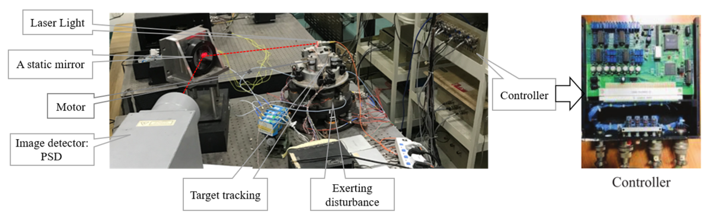
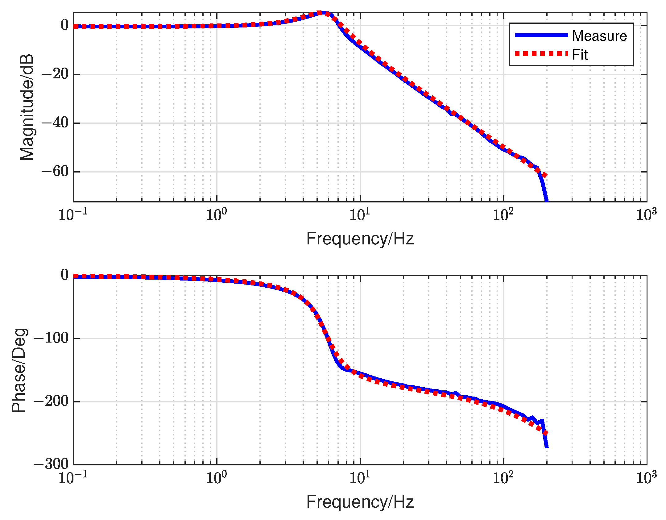
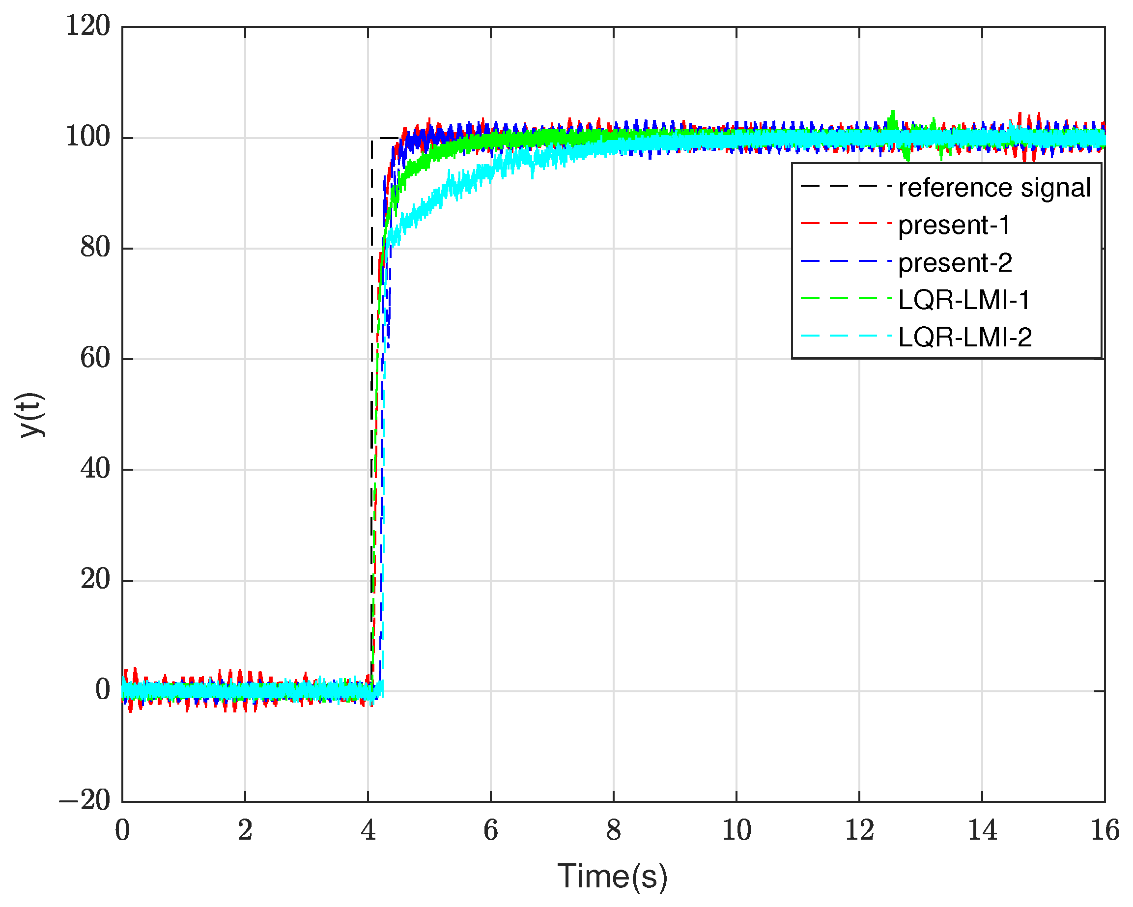
3.2. The Experiment Part of the High-Type Control Loop

The electro-optical tracking platform in Figure 13 is a device that captures target information in real time through an optical sensor PSD (Position Sensitive Detector) and uses a servo control system to drive mechanical structures for automatic target tracking.
Through sweep frequency analysis in Figure 14, the object transfer function fitting is
G ( s ) = 66970 37.7 s 2 + 966.4 s + 53580 .
The controllers (Equations (42) and (47)) under the method proposed in this paper, the controllers (Equations (44) and (49)) under the LQR method and the controllers (Equations (43) and (48)) under the LQR-LMI method are applied to the experimental system in Figure 13. Compared with the LQR method and LQR-LMI method in Figure 15 and Figure 16, the proposed method has significantly improved the dynamic response performance and disturbance suppression ability of the system. In general, the experimental verification proves the superiority and effectiveness of the high-type control loop design method for LQR-LMI based on Lyapunov and polyhedral model theory.
To highlight the role of the polyhedral model theory in the proposed method (resistance to internal parameter perturbation), the response under the proposed method and the LQR-LMI method are compared in Figure 17. Figure 17 shows the comparison of response between the proposed method and LQR-LMI method when the natural frequency changes. Present-1 represents the response curve of the proposed method under the natural frequency of 33.9 Hz. Present-2 represents the response curve of the proposed method under the natural frequency of 31.9 Hz. LQR-LMI-1 represents the response curve of the LQR-LMI method under the natural frequency of 33.9 Hz. LQR-LMI-2 represents the system response curve of the LQR-LMI method under the natural frequency of 31.9 Hz. By comparing the curves of present-1, present-2 and LQR-LMI-1, LQR-LMI-2, the response under the proposed method (present-1, present-2) is almost not affected by the internal parameter perturbation. Moreover, compared with the LQR-LMI method, the proposed method has improved the dynamic response of system, which shows the effectiveness of introducing the polyhedral model theory.

4. Conclusions and Future Outlook

The high-type control loop design method for LQR-LMI based on Lyapunov and polyhedral model theory is proposed. The high-type control loop design problem is simplified into a convex constraint problem, which achieves higher tracking accuracy and stronger disturbance suppression ability. And the problem that the LQR method is difficult to solve under various constraints has been solved through the LMI technology. Another point of innovation of this paper lies in characterizing the uncertainty of the system through the polyhedral control theory, achieving a good suppression of the system uncertainty. Considering the issue of efficient control of the actual system under interference factors, while reducing the frequency of data transmission or sampling and lowering the consumption of communication/computing resources, the next step after this paper will be to discuss the discrete-time event-triggered H-infinity stabilization for three closed-loop cyber-physical system with uncertain delay.

Author Contributions

Conceptualization, C.L., X.Q. and Y.M.; Methodology, C.L.; Software, C.L. and X.Q.; Validation, C.L. and X.Q.; Formal analysis, C.L. and X.Q.; Investigation, C.L.; Resources, Y.M.; Data curation, C.L. and X.Q.; Writing—original draft, C.L. and X.Q.; Writing—review and editing, C.L.; Visualization, C.L. and X.Q.; Supervision, C.L. and Y.M.; Project administration, C.L. and Y.M.; Funding acquisition, Y.M. All authors have read and agreed to the published version of the manuscript.

Funding

This work was supported in part by the National Natural Science Foundation of China (No. 61905253). We acknowledge funding from the National Natural Science Foundation.

Data Availability Statement

Research data are not shared. The data presented in this study are available on request from the author.

Conflicts of Interest

The authors declared no potential conflicts of interest with respect to the research, authorship, and/or publication of this article.

References

  1. Deng, J.; Xue, W.; Zhou, X.; Mao, Y. On dual compensation to disturbances and uncertainties for inertially stabilized platforms. Int. J. Control Autom. Syst. 2022, 20, 1521–1534. [Google Scholar] [CrossRef]
  2. Zhou, X.; Mao, Y.; Duan, Q.; Zhang, H. Multi-order cascade lag control for high precision tracking systems. ISA Trans. 2022, 120, 318–329. [Google Scholar] [CrossRef] [PubMed]
  3. Liu, C.; Mao, Y.; Qiu, X. Disturbance-observer-based LQR tracking control for electro-optical system. Photonics 2023, 10, 900. [Google Scholar] [CrossRef]
  4. Duan, Q.; Zhou, X.; He, Q.; Chen, X.; Liu, W.; Mao, Y. Pointing control design based on the PID type-III control loop for two-axis gimbal systems. Sens. Actuators A Phys. 2021, 331, 112923. [Google Scholar] [CrossRef]
  5. Chen, P.; Zhang, Y.; Wang, J.; Azar, A.T.; Hameed, I.A.; Ibraheem, I.K.; Kamal, N.A.; Abdulmajeed, F.A. Adaptive internal model control based on parameter adaptation. Electronics 2022, 11, 3842. [Google Scholar] [CrossRef]
  6. Chen, C.-W.; Wu, H.-M.; Nian, C.-Y. A Class of Anti-Windup Controllers for Precise Positioning of an X-Y Platform with Input Saturations. Electronics 2025, 14, 539. [Google Scholar] [CrossRef]
  7. Behnamgol, V.; Asadi, M.; Aphale, S.S.; Sohani, B. Recursive PID-NT Estimation-Based Second-Order SMC Strategy for Knee Exoskeleton Robots: A Focus on Uncertainty Mitigation. Electronics 2025, 14, 1455. [Google Scholar] [CrossRef]
  8. Tran, G.Q.B.; Pham, T.-P.; Sename, O.; Costa, E.; Gaspar, P. Integrated comfort-adaptive cruise and semi-active suspension control for an autonomous vehicle: An LPV approach. Electronics 2021, 10, 813. [Google Scholar] [CrossRef]
  9. Wang, T.; Wang, X. Polytopic Model Weighted Hoo Output Feedback Control of Switched Lpv System Based on Mdadt. J. Phys. Conf. Ser. 2019, 1267, 012089. [Google Scholar] [CrossRef]
  10. Tang, W.; Li, B.; Hou, S.; Shao, X.; Yu, H. Transient Stability Analysis for Grid-Connected Renewable Power Generation Systems Based on LMI Optimization Modelling. Electronics 2024, 13, 5052. [Google Scholar] [CrossRef]
  11. Song, R.; Huang, S.; Xiong, L.; Zhou, Y.; Li, T.; Tan, P.; Sun, Z. Takagi–Sugeno Fuzzy Parallel Distributed Compensation Control for Low-Frequency Oscillation Suppression in Wind Energy-Penetrated Power Systems. Electronics 2024, 13, 3795. [Google Scholar] [CrossRef]
  12. İnci, M.; Altun, Y. Disturbance compensator design based on dilated lmi for linear parameter-varying systems. Electronics 2024, 13, 3055. [Google Scholar] [CrossRef]
  13. Gao, J.; Li, H. Tuning Parameters of the Fractional Order PID-LQR Controller for Semi-Active Suspension. Electronics 2023, 12, 4115. [Google Scholar] [CrossRef]
  14. Rauniyar, S.; Bhalla, S.; Choi, D.; Kim, D. EKF-SLAM for quadcopter using differential flatness-based LQR control. Electronics 2023, 12, 1113. [Google Scholar] [CrossRef]
  15. Mosavi, A.; Qasem, S.N.; Shokri, M.; Band, S.S.; Mohammadzadeh, A. Fractional-order fuzzy control approach for photovoltaic/battery systems under unknown dynamics, variable irradiation and temperature. Electronics 2020, 9, 1455. [Google Scholar] [CrossRef]
  16. Wang, S.; Yu, F.; Qi, J. Model Predictive Voltage Control Strategy for Dual Active Bridge Converters Based on Super-Twisting Integral Sliding Mode Observer. Electronics 2025, 14, 1496. [Google Scholar] [CrossRef]
  17. Liu, C.; Qiu, X.; Xu, T.; Wei, W.; Sun, H.; Hou, Y. A Linear Quadratic Regulation Controller Based on Radial Basis Function Network Approximation. Electronics 2024, 13, 4279. [Google Scholar] [CrossRef]
  18. da Ponte Caun, R.; Assunção, E.; Minhoto Teixeira, M.C. H2/H formulation of LQR controls based on LMI for continuous-time uncertain systems. Int. J. Syst. Sci. 2021, 52, 612–634. [Google Scholar] [CrossRef]
  19. Liu, C.; Qiu, X.X.; Mao, Y. The PID high-type controller based on LQR and model-assisted LESO. Proc. Inst. Mech. Eng. Part I J. Syst. Control Eng. 2025, 239, 74–89. [Google Scholar] [CrossRef]
  20. Papadopoulos, K.G.; Papastefanaki, E.N.; Margaris, N.I. Optimal tuning of PID controllers for type-III control loops. In Proceedings of the 2011 19th Mediterranean Conference on Control & Automation (MED), Corfu, Greece, 20–23 June 2011; pp. 1295–1300. [Google Scholar]
  21. Deng, J.; Meng, X.; Jiang, B. Observer-Based Robust Hoo Control for Stochastic Markov Jump Delay Systems Through Dual Adaptive Sliding Mode Approach. Electronics 2024, 14, 132. [Google Scholar] [CrossRef]
  22. Kim, C. Robust Hoo Static Output Feedback Control for TCP/AQM Routers Based on LMI Optimization. Electronics 2024, 13, 2165. [Google Scholar] [CrossRef]
  23. Duan, G.R.; Yu, H.H. LMIs in Control Systems: Analysis, Design and Applications; CRC Press: Boca Raton, FL, USA, 2013. [Google Scholar]
  24. Belov, A.A. State-feedback anisotropy-based robust control of linear systems with polytopic uncertainties. J. Phys. Conf. Ser. 2020, 1536, 012008. [Google Scholar] [CrossRef]
  25. Ding, W.; Li, W.; Qiao, J. Anti-Disturbance Multi-Objective H2/H Fusion Scheme for End-Effector Position Estimation of Space Manipulator. In Proceedings of the 2021 33rd Chinese Control and Decision Conference (CCDC), Kunming, China, 22–24 May 2021; pp. 7265–7271. [Google Scholar]
  26. Sereni, B. Two-Stage Static Output Feedback Controller Design for Linear Systems Under LMI Pole Placement and H2/H Guaranteed Cost Constraints. Ph.D. Thesis, São Paulo State University, São Paulo, Brazil, 2023. [Google Scholar]
  27. Wu, H.N.; Zhu, H.Y.; Wang, J.W. Hoo Fuzzy Control for a Class of Nonlinear Coupled ODE-PDE Systems with Input Constraint. IEEE Trans. Fuzzy Syst. 2014, 23, 593–604. [Google Scholar] [CrossRef]
Figure 1. The H 2 / H control structure block diagram.
Electronics 14 02491 g001
Figure 2. The design principle of type-ii control loop.
Electronics 14 02491 g002
Figure 3. The design principle of type-iii control loop.
Electronics 14 02491 g003
Figure 4. (a) and (b) are the step response and controller response under 50 % disturbance at t = 20 s, respectively.
Electronics 14 02491 g004
Figure 5. (a) and (b) are the step response and controller response under the LQR-LMI method, respectively; (c) and (d) are the step response and controller response under the proposed method, respectively.
Electronics 14 02491 g005
Figure 6. The tracking response under the proposed type-ii control method. (a) shows the tracking response and tracking error of sin(0.1t), sin(t) and sin(10t) under the proposed type-ii control method, respectively. (b) shows the controller response of sin(0.1t), sin(t) and sin(10t) under the proposed type-ii control method, respectively.
Electronics 14 02491 g006
Figure 7. (a) and (b) are the response of system and controller under 50 % disturbance at t = 40 s in the type-iii control loop, respectively.
Electronics 14 02491 g007
Figure 8. (a) and (b) are the response of system and controller under the LQR-LMI method in the type-iii control loop, respectively; (c) and (d) are the response of system and controller response under the proposed type-iii control method, respectively.
Electronics 14 02491 g008
Figure 9. The tracking response under the proposed type-iii control method. (a) shows the tracking response and tracking error of sin(0.1t), sin(t) and sin(10t) under the proposed type-iii control method, respectively. (b) shows the controller response of sin(0.1t), sin(t) and sin(10t) under the proposed type-iii control method, respectively.
Electronics 14 02491 g009
Figure 10. (a) and (c) are the tracking response of velocity and acceleration signals, respectively. (b) and (d) are the tracking error of velocity and acceleration signals, respectively.
Electronics 14 02491 g010
Figure 11. The response of system and controller in the type-ii control loop under different methods.
Electronics 14 02491 g011
Figure 12. The response of system and controller in the type-iii control loop under different methods.
Electronics 14 02491 g012
Figure 13. The experimental platform.
Electronics 14 02491 g013
Figure 14. The characteristic of the controlled plant.
Electronics 14 02491 g014
Figure 15. The comparison diagram of system response under step disturbance in the type-ii control loop.
Electronics 14 02491 g015
Figure 16. The comparison diagram of system response under step disturbance in the type-iii control loop.
Electronics 14 02491 g016
Figure 17. The comparison diagram of system response under the change of plant.
Electronics 14 02491 g017
Disclaimer/Publisher’s Note: The statements, opinions and data contained in all publications are solely those of the individual author(s) and contributor(s) and not of MDPI and/or the editor(s). MDPI and/or the editor(s) disclaim responsibility for any injury to people or property resulting from any ideas, methods, instructions or products referred to in the content.

