RMSENet: Multi-Scale Reverse Master–Slave Encoder Network for Remote Sensing Image Scene Classification

Abstract

Aiming at the problems that the semantic representation of information extracted by the shallow layer of the current remote sensing image scene classification network is insufficient, and that the utilization rate of primary visual features decreases with the deepening of the network layers, this paper designs a multi-scale reverse master–slave encoder network (RMSENet). It proposes a reverse cross-scale supplementation strategy for the slave encoder and a reverse cross-scale fusion strategy for the master encoder. This not only reversely supplements the high-level semantic information extracted by the slave encoder to the shallow layer of the master encoder network in a cross-scale manner but also realizes the cross-scale fusion of features at all stages of the master encoder. A multi-frequency coordinate channel attention mechanism is proposed, which captures the inter-channel interactions of input feature maps while embedding spatial position information and rich frequency information. A multi-scale wavelet self-attention mechanism is proposed, which completes lossless downsampling of input feature maps before self-attention operations. Experiments on open-source datasets RSSCN7, SIRI-WHU, and AID show that the classification accuracies of RMSENet reach 97.41%, 97.61%, and 95.9%, respectively. Compared with current mainstream deep learning models, RMSENet has lower network complexity and excellent classification accuracy.

1. Introduction

With the rapid development of remote sensing observation technology, remote sensing image data are increasing [1]. The remote sensing image scene classification (RSSC) task has become a key research field of computer vision, involving the assignment of image-corresponding semantic tags based on image content. RSSC is widely used in natural disaster detection, land use, urban planning and other fields [2]. With the increasing spatial resolution of remote sensing images, more and more categories are covered, and the categories affect each other. For different images of the same category, it is easy to classify different images that originally belong to the same category into different categories due to their different details. For images of different categories, their image features may have a high degree of similarity, which may easily lead to images originally belonging to different categories being wrongly summarized into the same category. A series of factors, such as the diversity of landforms and the complexity of spatial distribution involved, have brought challenges to the task of RSSC [3]. The classification error of remote sensing image can easily cause the misjudgment of natural disaster types, statistical deviation of land use resources, unreasonable urban planning and design, and other impacts. Therefore, it is of great significance to carry out research and an investigation on RSSC and design a RSSC model with excellent performance.

Due to the powerful feature extraction capabilities and weight-sharing properties of CNNs, a series of CNN-based models have achieved remarkable success in the field of deep learning [4,5]. However, it is difficult for CNNs to establish long-distance feature dependency, which easily causes the loss of high-level semantic information of remote sensing images. Transformers [6] have not only achieved remarkable success in the field of natural language processing but have also been widely applied in the field of computer vision [7,8]. However, due to the lack of natural inductive bias, such as local correlation and translation invariance, their generalization is insufficient. At present, combining the advantages of CNNs and Transformers is the mainstream idea in designing the RSSC model. However, the RSSC models based on the hybrid architecture of CNNs and Transformers only simply stack convolution and Transformers, use convolution to extract shallow texture information from the shallow layer of the network, and use Transformers to extract high-level semantic information from the deep layer of the network. To some extent, they combine the advantages of CNN and Transformer architecture but ignore the cross-scale fusion of features extracted at each stage of the network and the supplement of high-level semantic information to the shallow layer of the network, which is of great significance to make full use of local texture information and enhance the network’s ability to understand the input feature map at multiple levels.

In view of the above problems, this paper designs a multi-scale reverse master–slave encoder network RMSENet. Combining the advantages of CNNs and Transformers, it focuses on the extraction and fusion of image information and designs a reverse cross-scale fusion strategy for the master encoder and a reverse cross-scale supplement strategy for the slave encoder, along with a local information extraction module and a local global information parallel extraction module. The main contributions of this paper are summarized as follows:

1.

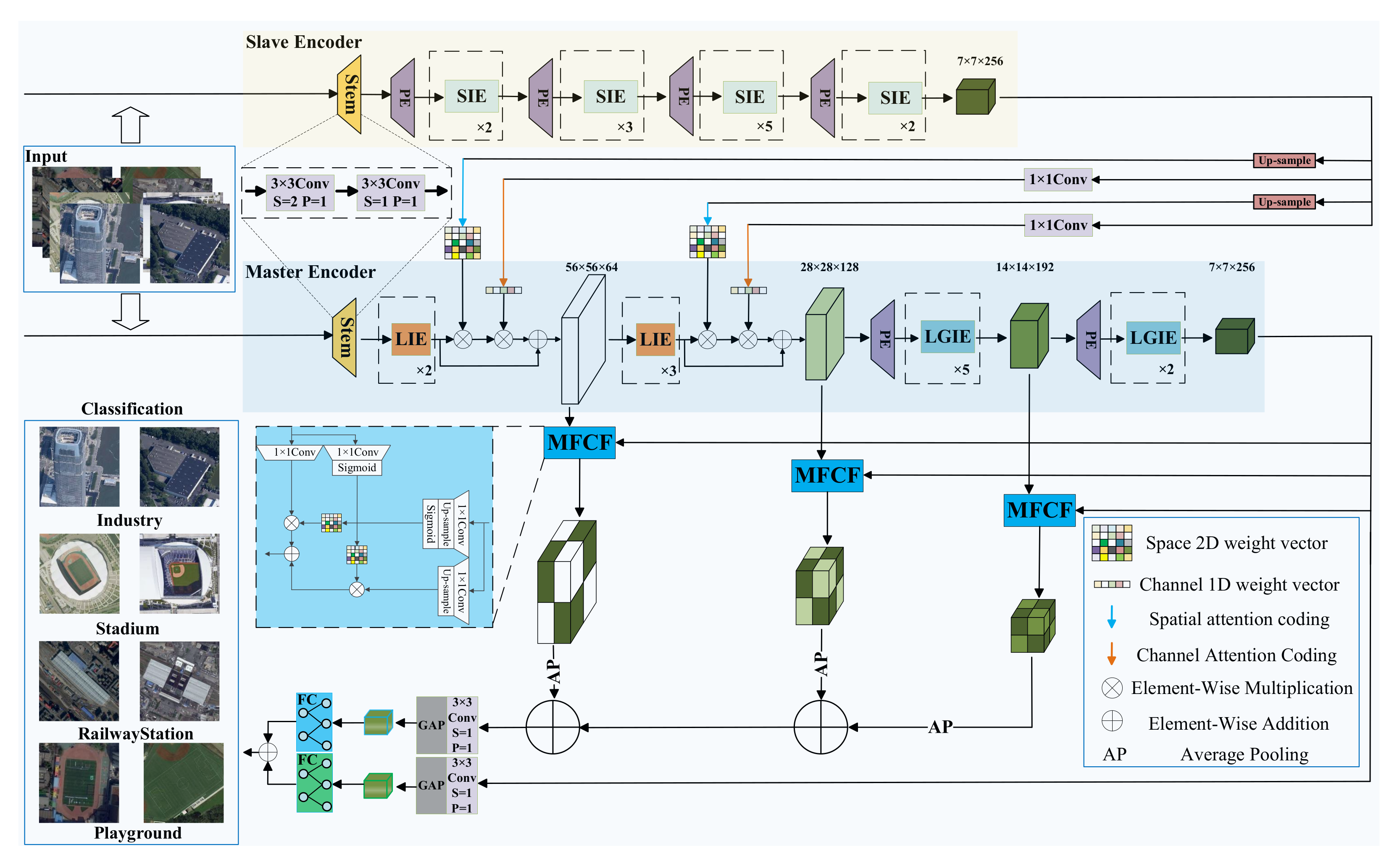
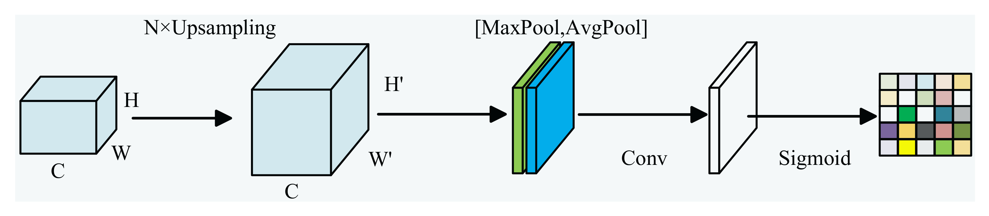
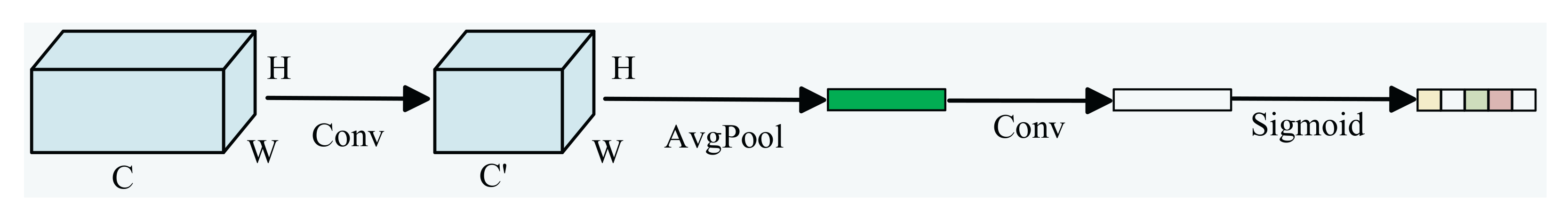
A reverse cross-scale fusion strategy for the master encoder and a reverse cross-scale supplementation strategy for the slave encoder were designed, which not only fused the features extracted from each stage of the master encoder cross-scale but also supplemented the high-level semantic information output from the slave encoder to the shallow stage of the master encoder network, effectively guided the feature extraction of the image in each stage of the master encoder network, and enhanced the multi-level understanding ability of the network to the input image.

2.

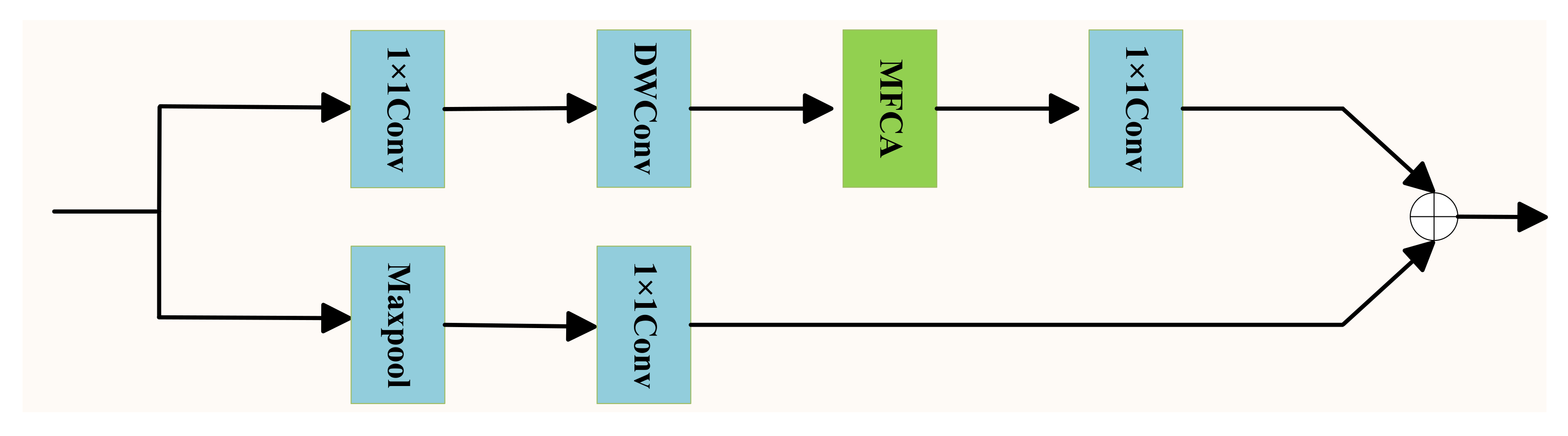
The local information extraction module is designed. In this module, multi-frequency coordinate channel attention is proposed. According to the importance of each channel in the feature map, weight distribution is given and spatial position information and rich frequency information are embedded at the same time, which effectively improves the feature extraction ability of remote sensing images.

3.

The local global information parallel extraction module is designed. In this module, the local global information parallel extraction and cross-fusion are realized. The multi-scale wavelet self-attention is proposed. Before the self-attention calculation, the wavelet transform is used to complete the downsampling of the input feature map, and the information loss caused by the downsampling is compensated by the inverse wavelet transform, so as to realize the lossless downsampling.

4.

Based on the above design module, RMSENet is proposed. The experimental results show that the classification performance of RMSENet on RSSCN7, AID and SIRI-WHU datasets has certain advantages over other classification models.

2. Related Work

This chapter mainly introduces the related work on CNN-based architecture models, Transformer-based architecture models, hybrid architecture models combining CNNs and Transformers, and model encoder structure design in remote sensing scene classification (RSSC) models.

2.1. CNN-Based RSSC Models

CNNs excel at processing two-dimensional image data and are widely used in the field of image classification. AlexNet [9] was the first to apply CNNs to large-scale image classification tasks, significantly improving classification accuracy. ResNet [10] introduced residual connections to address the problems of gradient disappearance and explosion in deep neural network training. DenseNet [11] achieved excellent classification performance in RSSC tasks by adaptively enhancing the weights of important feature channels. Finder et al. [12] proposed WTConv, which achieves a larger receptive field while avoiding the problem of parameter explosion. Cheng et al. [13] integrated band information of different resolutions through a multi-spectral stacking module, enhancing the feature extraction capability for high-resolution remote sensing images. These CNN-based architecture models are good at extracting local features but have weak capabilities for modeling long-range dependencies in images and thus struggle to capture some global semantic information in images.

2.2. Transformer-Based RSSC Models

Transformers demonstrate remarkable potential in RSSC tasks. Dosovitskiy et al. [14] proposed ViT, which uses image patch partitioning to prove that Transformers can achieve excellent performance in image tasks on large-scale datasets. Swin Transformer [15] introduces a hierarchical Transformer structure and shift window mechanism, enhancing the model’s ability to handle visual entities of different scales. Lv et al. [16] developed SCViT, which retains spatial structure information and channel features in high-resolution remote sensing images through a progressive aggregation strategy and lightweight channel attention module. S4Former [17] applies the deep unfolding method from sparse coding to ViT, enhancing the model’s capability to capture sparse and key features by gradually optimizing token representations. Zhang et al. [18] proposed CAS-ViT, which eliminates complex matrix operations and softmax through a convolutional additive self-attention mechanism (CATM), significantly reducing computational costs. While these Transformer-based architectures excel at capturing long-range dependencies between image pixels, they have limited local information processing capabilities and poor adaptability to input image resolution.

2.3. Hybrid CNN-Transformer Architecture Models for RSSC

Currently, an increasing number of hybrid architecture models based on CNNs and Transformers have emerged. CoAtNet [19] proposes a network architecture with vertical stacking of convolutional layers and self-attention layers, combining the advantages of both to achieve excellent performance across different datasets. Xu et al. [20] developed DBCTNet, which designs a convolution-enhanced Transformer encoder to reduce model complexity while maintaining the ability to extract spectral features from remote sensing images. Hybrid FusionNet [21] integrates 2D–3D convolutional neural networks with Transformer encoders, effectively fusing multi-dimensional features of remote sensing images to achieve accurate classification of complex objects even with limited training data. However, these hybrid CNN-Transformer architectures currently fail to consider the importance of spatial position information and frequency information while capturing interactions between feature map channels. Additionally, although downsampling before self-attention calculation can reduce computational complexity, it inevitably leads to information loss.

2.4. The Encoder Structure for RSSC

Currently, the mainstream encoding structure for RSSC models is the single-branch architecture, where remote sensing images are input into a single feature extraction network to extract image features. Models such as AlexNet, VGGNet [22], ResNet, Vision Transformer, Swin Transformer, CoAtNet, and DBCTNet all adopt this single-branch encoding structure. In contrast to single-branch architectures, dual-branch encoding structures can avoid homogeneous feature extraction and effectively enhance model robustness by combining the outputs of different encoders. For example, Deng et al. [23] proposed the dual-branch network CTNet, which uses CNN and ViT to extract structural and semantic features of remote sensing images, respectively, thereby improving the model’s recognition capability for such images. Yang et al. [24] achieved high-precision and efficient scene classification by introducing a local–global (LG) adaptive feature extractor and a global feature learning mechanism. Yue et al. [25] designed an auxiliary enhancement unit (AEU) and an interactive perception unit (IPU) to fuse features extracted by two encoders, effectively enhancing the feature discriminability in remote sensing scene classification. However, current RSSC models with dual-branch encoding structures suffer from insufficient scene-level semantic capabilities in the information extracted by the shallow network layers. Additionally, they overlook the fusion of features extracted at different network stages, leading to inadequate multi-level understanding of input images.

3. Methods

In the task of remote sensing image scene classification (RSSC), it is very important to correctly model the underlying semantic information, background information, and dependencies between objects. For example, to achieve the correct classification of industrial park scenes, two conditions need to be met: first, the scene must contain factory buildings with diverse characteristics; secondly, they must be widely distributed across the image. Therefore, when extracting features from remote sensing images, it is necessary to pay attention to both local and global features. The extraction of local features can capture the details of objects, such as the shape and color of factory buildings. The extraction of global features can reflect the structure and distribution of the scene. At the same time, the high-level semantic information is added to the shallow stage of the model network, so that the extracted information has the scene level semantic ability, which can accelerate the model learning process, enhance the generalization ability, and improve the accuracy of RSSC.

3.1. Overall Architecture

Aiming at the characteristics of rich texture information and complex overall structure of remote sensing images, this paper designs a multi-scale reverse master–slave encoder network (RMSENet) for RSSC. The overall architecture of RMSENet is shown in Figure 1. First, preprocess the input image and then input the image to the slave encoder and the master encoder, respectively. The purpose of the Stem is to reduce redundancy by halving the size of the input feature map when extracting shallow features, while increasing the number of channels to increase feature capacity. The slave encoder consists of four stages and an external supplementary branch. Each stage consists of a semantic information extraction module (SIE), which is used to extract the high-level semantic information of the image. At the same time, a collaborative mechanism of cross-scale spatial attention coding and cross-scale channel attention coding is designed to realize the reverse cross-scale supplement of high-level semantic information output from the slave encoder to the shallow network stage of the master encoder, so that the master encoder can obtain the feature map with high-level semantic representation earlier in each network stage. The master encoder consists of four stages and an external fusion branch. The first two stages are local information extraction module (LIE), which is used to extract shallow texture information. The last two stages are the local global information extraction module (LGIE), which extracts local information and global information in parallel and then conducts cross-fusion. The external fusion branch of the master encoder cross-fuses the output of the fourth stage of the master encoder with the output of the first three stages to enrich the multi-scale features, further uses the edge, texture and other features extracted in the shallow stage, and finally outputs the results through a hybrid classification output module. The PE is a convolution operation with a kernel size of 3 and a stride of 2. Its purpose is to downsample the input feature map to reduce redundancy and increase the channels by 64 to enrich features.

3.2. Slave Encoder

This section details the constituent modules of the slave encoder and expounds on how the high-level semantic information extracted by the slave encoder is reversely supplemented across scales to the shallow stages of the master encoder network. Specifically, Section 3.2.1 introduces the semantic information extraction (SIE) module within the slave encoder, and Section 3.2.2 describes the reverse cross-scale supplementation strategy for the slave encoder.

3.2.1. SIE Module

In the slave encoder, this paper has designed a SIE module. The details of the SIE module are shown in Figure 2. Considering that multi-scale information helps the network extract objects or structures of different sizes, the network can better adapt to complex scenes and improve the robustness of the network. In this paper, the feature maps of key vectors and value vectors are divided according to channels, and then they are concatenated along the channel direction after being processed by depthwise convolutions with different receptive fields. Subsequently, the keys and values are obtained through a linear layer. The query vector Q is directly obtained from the input through a linear layer; finally, semantic information is extracted through multi-head self-attention. Assume the input of the SIE module is $X_{SIE}\in {\mathbb{R}}^{H\times W\times C}$; the output of self-attention is shown in Equations (1) and (2):

$$X_1,X_2,\dots ,X_n=C_{-}Split\left(X_{SIE}\right),X_i^{\prime }=D{W}^{(2i-1)\times (2i-1)}\left(X_i\right)\cdots i\in \{1,\dots ,n\}$$

(1)

$$F=Concat(X_1^{\prime },X_2^{\prime },\dots ,X_n^{\prime }),Attention=softmax\left({\displaystyle \frac{\left(W^Q{X}_{SIE}\right){\left(W^{K}F\right)}^T}{\sqrt{D}}}\right)\left(W^{V}F\right)$$

(2)

Here, $C_{-}Split$ denotes the average division of the input feature map $X_{SIE}$ along the channel direction into n equal parts, where n in the SIE is set to 4. ${DW}^{(2i-1)\times (2i-1)}(·)$ represents depthwise convolution with a kernel size of $(2i-1)\times (2i-1)$ and a stride of 2. The matrices $W^Q\in {\mathbb{R}}^{C\times C},W^K\in {\mathbb{R}}^{C\times C},W^V\in {\mathbb{R}}^{C\times C}$ denote projection matrices. $Concat$ denotes concatenation along the channel dimension; D denotes the channel dimension of keys and values. Self-attention operations primarily capture low-frequency information and have limited ability to learn high-frequency information. Max pooling emphasizes significant features in the input by retaining the maximum values in local regions. The SIE extracts low-frequency information through self-attention operations, in parallel with max pooling and $1\times 1$ convolution to capture high-frequency information, and then fuses it with the low-frequency information branch by addition.

3.2.2. Reverse Cross-Scale Supplementation Strategy for the Slave Encoder

The features extracted in depth from the network contain rich high-level semantic information, representing the abstract information of the entire image. The features extracted from the shallow layer of the network reflect the details of the image and contain more local information but lack high-level semantic information. By reverse cross-scale supplementation the high-level semantic information extracted from the deep layer of the slave encoder network to the shallow layer of the master encoder network, the master encoder network structure can be optimized; therefore, the feature map with high-level semantic representation can be obtained earlier in each network stage of the master encoder, promoting the integration of low-level features and high-level semantic information, thus generating feature representations rich in abstract semantics at the initial stage of the coding process and enhancing the network’s multi-level understanding ability of input image. As shown in Figure 1, first of all, the feature maps output from the last stage of the slave encoder are, respectively, subjected to cross-scale spatial attention coding to generate spatial two-dimensional weight vectors and cross-scale channel attention coding to generate channel one-dimensional weight vectors, which are multiplied with the output of the master encoder’s LIE module in turn. At the same time, a shortcut branch is added to avoid the loss of original information. Cross-scale spatial attention coding is shown in Figure 3. First, the feature map is upsampled, the global average pooling and global maximum pooling are performed along the channel, and then the two are spliced and output through convolution and activation function. Cross-scale channel attention coding is shown in Figure 4. First, the feature map is convolved with a convolution kernel size of 1 × 1, the global average pooling is performed along the spatial direction, and then output through convolution and activation function. Assuming that the output of the slave encoder is $Y_{Slave}\in {\mathbb{R}}^{H\times W\times C}$, the process of cross-scale spatial attention coding and cross-scale channel attention coding is shown in Equations (3) and (4), where ↑ denotes upsampling, $Gap(·)$ denotes global average pooling, and $Gmp(·)$ denotes global max pooling. $C^{i\times i}(·)$ denotes a regular convolution with a $i\times i$ kernel. $\sigma (·)$ denotes the sigmoid activation function.

$$Y_{SAE}=\sigma \left(C^{7\times 7}\left(Concat\left(Gap(Y_{Slave}\uparrow ),Gmp(Y_{Slave}\uparrow )\right)\right)\right)$$

(3)

$$Y_{CAE}=\sigma \left(C^{1\times 1}\left(Gap\left(C^{1\times 1}\left(Y_{Slave}\right)\right)\right)\right)$$

(4)

3.3. Master Encoder

This section details the constituent modules of the master encoder and elaborates on the cross-scale cross-fusion of outputs from the fourth stage of the master encoder with outputs from the first three stages. This approach leverages local texture information extracted from shallow network stages to enhance feature representation. Specifically, Section 3.3.1 introduces the local information extraction (LIE) module within the master encoder, Section 3.3.2 describes the local and global information extraction (LGIE) module of the master encoder, and Section 3.3.3 presents the backward cross-scale fusion strategy of the master encoder.

3.3.1. Local Information Extraction (LIE) Module

In the shallow layer of the master encoder network, this paper designs an LIE module, which adopts a pure convolution mode and designs a parallel structure of two branches, aiming to extract shallow texture information, which can provide rich visual representation. First, the number of channels input to the feature map is expanded by four times through a $1\times 1$ convolution. Then, a depthwise convolution with a convolution kernel size of $3\times 3$ is used to extract local features. Since the modeling ability of depth convolution in channel dimension is limited, the feature map after depthwise convolution will proceed through multi-frequency coordinate channel attention (MFCA) to capture the interaction between channels and finally recover the original channel number through $1\times 1$ convolution. The first and second stages of the master encoder stack two and three LIE modules, respectively. When the feature map is input into the first LIE module, it is downsampled twice and matched with the dimension through the maximum pooling and convolution on the other branch, as shown in Figure 5. When the feature map is input into the $3\times 3$ depthwise convolution in the second and third LIE modules, the downsampling is not performed, and the shortcut branch is used instead of the maximum pooling and convolution operation. Assume the input of the LIE module is $X_{LIE}\in {\mathbb{R}}^{H\times W\times C}$; the output of LIE module is shown in Equation (5). The multi-frequency coordinate channel attention is shown in Figure 6. The spatial position information is obtained through the global dependency modeling of the input feature map along the height and width directions. At the same time, channel segmentation is performed on the input feature map, and two-dimensional discrete cosine transform is performed on each channel of the feature map to obtain rich frequency information. Finally, multiply the input feature map by the results output from the two operations mentioned above, and each channel is given different weights to enhance the global context understanding ability of features and enrich the frequency information. Assuming that the input of the MFCA is $X_{MFCA}\in {\mathbb{R}}^{H\times W\times C}$, the output of MFCA is shown in Equations (6)–(10).

$$Y_{LIE}=C^{1\times 1}\left(MFCA\left(D{W}^{3\times 3}\left(C^{1\times 1}\left(X_{LIE}\right)\right)\right)\right)+C^{1\times 1}\left(M_p\left(X_{LIE}\right)\right)$$

(5)

$$X_C^{\prime }=BN\left(C^{1\times 1}\left(Concat(W_{-}{A}_{-}P\left(X_{MFCA}\right),H_{-}{A}_{-}P\left(X_{MFCA}\right))\right)\right)$$

(6)

$$X_{C1}^{\prime },X_{C2}^{\prime }=H_{-}Split\left(X_C^{\prime }\right),X_0^{\prime },X_1^{\prime },\dots ,X_{n-1}^{\prime }=C_{-}Split\left(X_{MFCA}\right)$$

(7)

$${Freq}^i=2{DDCT}^i\left(X_i^{\prime }\right)=\sum _{h=0}^{H-1}\sum _{w=0}^{W-1}{X}_{ih,w}^{\prime }{\beta }_{h,w}^{u_i}i\in \{0,1,\dots ,n-1\}$$

(8)

$$Freq=Concat\left([{Freq}^0,{Freq}^0,\dots ,{Freq}^{n-1}]\right),M_{-}{S}_{-}A=\sigma \left(FC\left(Freq\right)\right)$$

(9)

$$Y_{MFCA}=X_{MFCA}\times C^{1\times 1}\left(X_{C1}^{\prime }\right)\times C^{1\times 1}\left(X_{C2}^{\prime }\right)\times M_{-}{S}_{-}A$$

(10)

where $C^{1\times 1}(·)$ denotes a convolution with a kernel size of $1\times 1$, $D{W}^{3\times 3}(·)$ denotes a depthwise convolution with a kernel size of $3\times 3$, $Mp(·)$ represents max pooling, $\sigma (·)$ represents the sigmoid activation function, $BN(·)$ represents batch normalization, $W\_A\_P(·)$ and $H\_A\_P(·)$, respectively, denote average pooling along the width and height directions of the feature map, $2DDCT$ is a two-dimensional discrete cosine transform, $\beta$ is the basis function of the two-dimensional discrete cosine transform, and $[u_i,v_i]$ are the 2D indices of the corresponding frequency components of $X_i^{\prime }$.

3.3.2. Local and Global Information Extraction (LGIE) Module

In the deep layer of the master encoder network, an LGIE module is designed. In this module, multi-scale wavelet self-attention module (MWSA) is proposed to extract the global features of the image. As shown in Figure 7, the LGIE module follows the general architecture of MetaFormer [26]. Due to the lack of inductive bias in the self-attention mechanism, it is easy to ignore some local details. Therefore, in the token mixer part, the MWSA module is used to extract global features, while a local feature extraction branch is paralleled to supplement local information. Finally, the global feature weight and local feature weight are generated by using the activation function, which are, respectively, multiplied by the output of the local feature extraction branch and the output of the global feature extraction branch. Then, the two outputs after the multiplication are multiplied again, and the feature representation is strengthened by 1 × 1 convolution, forming the cross-fusion of global features and local features. Specifically, in the token mixer part, a local global dual-branch feature extraction module is designed, which combines convolution and multi-scale wavelet self-attention. For the local feature extraction branch, the depthwise convolution is used to extract the local features of the image, and the activation function is used to generate weights to achieve self-modulation. The self-modulated feature map is used to capture the interaction between channels through the multi-frequency coordinate channel attention to enhance the information extraction ability. Finally, the activation function is used to generate the local feature weights and multiply the output of the global feature extraction branch. For the global feature extraction branch, an MWSA module is designed to extract the global features, and the wavelet transform is used to realize the downsampling. At the same time, the inverse wavelet transform is used to compensate for the information loss caused by the downsampling. The details of the MWSA module are shown in Figure 8. The input feature map is divided into channels. After the depthwise convolution of different receptive fields, they are spliced along the channel direction to capture multi-scale features. The feature map is downsampled using two-dimensional discrete wavelet transform, and then the key vector and value vector are generated through the linear layer. The query vector Q is directly obtained from the input through a linear layer. After Q, K, and V are used to perform multi-head self-attention operations, the information loss caused by the downsampling operation is compensated by inverse wavelet transform. The DWT selects the classic Haar [27] wavelet transform, and LL, LH, HL, and HH are the low-frequency sub-band, horizontal high-frequency sub-band, vertical high-frequency sub-band, and diagonal high-frequency sub-band of the image after discrete wavelet transform, respectively. Similar to the SIE module, the input feature map is passed through multi-scale wavelet self-attention; at the same time, it is paralleled to maximize pooling and 1 × 1 convolution to supplement high-frequency information.

Assuming that the input of the MWSA is $X_{MWSA}\in {\mathbb{R}}^{H\times W\times C}$, the output of MWSA module is shown in Equations (11)–(14), where $C_{-}split$ denotes the average division of the input feature map X along the channel direction into n equal parts to obtain $X_1,X_2,\dots ,X_n$, where n in the MWSA module takes $3,C^{1\times 1}(·)$ denotes a $1\times 1$ convolution kernel, and $D{W}^{(2i-1)(2i-1)}(·)$ represents a depthwise convolution kernel of size $(2i-1)\times (2i-1)$ with a stride setting of 1. Matrices $W^Q\in {\mathbb{R}}^{C\times C},W^K\in {\mathbb{R}}^{C\times C},W^V\in {\mathbb{R}}^{C\times C}$ represent projection matrices, $2DDWT$ denotes two-dimensional discrete wavelet transform, $IDWT$ represents inverse discrete wavelet transform. $Concat$ denotes concatenation along the channel dimension, and D represents the channel dimension of the keys and values.

$$X_1,X_2,\dots ,X_n=C_{-}split\left(X_{MWSA}\right),X_i^{\prime }=D{W}^{(2i-1)\times (2i-1)}\left(X_i\right)i\in \{1,\dots ,n\}$$

(11)

$$F=Concat(X_1^{\prime },X_2^{\prime },\dots ,X_n^{\prime }),LL,LH,HL,HH=2DDWT\left(F\right)$$

(12)

$$X^{\prime }=C^{1\times 1}\left(Concat(LL,LH,HL,HH)\right)$$

(13)

$$Attention=Concat\left(softmax\left({\displaystyle \frac{\left(W^Q{X}_{\mathrm{MWSA}}\right)\left(W^K{X}^{\prime T}\right)}{\sqrt{D}}}\right)\left(W^V{X}^{\prime }\right),IDWT\left(X^{\prime }\right)\right)$$

(14)

3.3.3. Reverse Cross-Scale Fusion Strategy for the Master Encoder

Research shows that with the increase in network layers, the model extracts more global semantic information from images. However, for remote sensing images with complex backgrounds, local texture information is the key to distinguish highly similar images. In this paper, a multi-scale feature cross-fusion module (MFCF) is designed to effectively use the local texture information extracted in the shallow stage to fully utilize the role of the extracted local texture information. As shown in Figure 1, the MFCF module mainly includes four parts, namely global weight, global features extracted in the network deep stage, local weight, and local features extracted in the network shallow stage. By cross-injecting local weight and global weight into global feature and local feature, respectively, and then adding the injected features, multi-scale feature cross-fusion is formed, which can fully extract global and local information while reducing the difference between features of different layers and further effectively use the local texture information. Specifically, take the local features generated in the first stage of the master encoder and the global features generated in the fourth stage of the master encoder as examples, assume that the input of the MFCF module from the first stage and the fourth stage is $X_{MFCF1}$ and $X_{MFCF4}$, respectively, and then pass $X_{MFCF1}$ through 1 × 1 convolution, batch normalization and sigmoid activation functions to obtain local weights. At the same time, $X_{MFCF1}$ is passed through a 1 × 1 convolutional, batch normalization generate local features. The $X_{MFCF4}$ is passed through a 1 × 1 convolutional, batch normalization, bilinear interpolation for upsampling, and a sigmoid activation function to obtain global weight. Meanwhile, $X_{MFCF4}$ is passed through a 1 × 1 convolutional and batch normalization; then, in another branch, bilinear interpolation upsampling is used twice to generate global features. Finally, the local weights and global weights are cross-injected into the global and local features through multiplication, and then the injected features are added together. The above process formula is described in Equation (15).

$$Y_{MFCF}=C^{1\times 1}\left(X_{MFCF1}\right)\times \sigma (C^{1\times 1}\left(X_{MFCF4}\right)\uparrow )+(C^{1\times 1}\left(X_{MFCF4}\right)\uparrow )\times \sigma \left(C^{1\times 1}\left(X_{MFCF1}\right)\right)$$

(15)

3.4. Classifier

As shown in Figure 1, the classifier module uses mixed classification output, integrating the deep features of the fourth stage of the master encoder and the contributions of multi-level features aggregated in each stage. In Equation (16), $Ou{t}_d$ is the classification score of deep features, and $Ou{t}_m$ is the classification score of multi-layer features.

$$Out=\left(Ou{t}_d+Ou{t}_m\right)/2$$

(16)

4. Experiment and Analysis

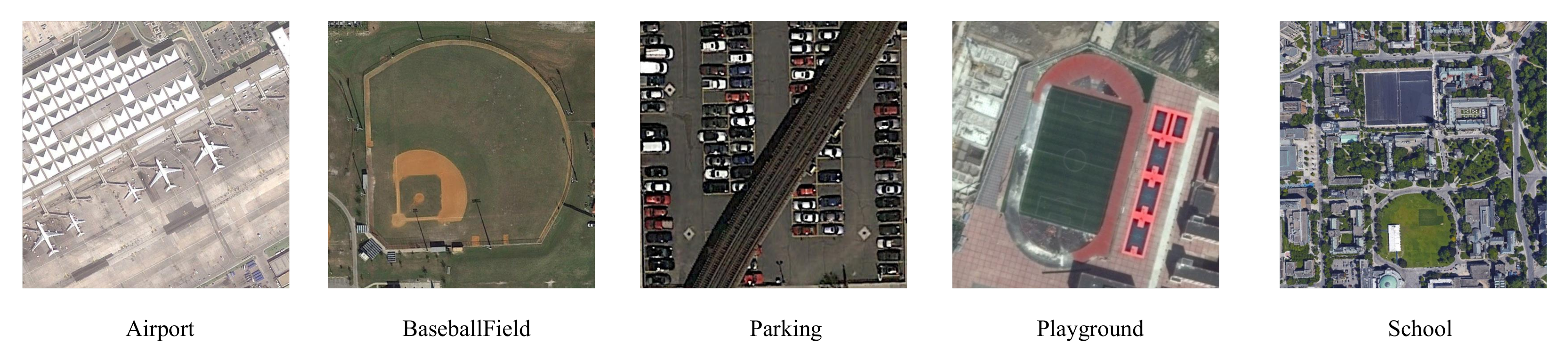
4.1. Dataset Introduction

The experiment employs three commonly used open-source remote sensing image datasets to evaluate the method proposed in this paper. The first is the RSSCN7 dataset [28], released in 2015, which contains a total of 2800 images across 7 scene categories. Each category comprises 400 RGB images of 400 × 400 pixels, with some example images shown in Figure 9. The second dataset is the AID dataset [29], released in 2017, which includes 30 scene categories with a total of 10,000 RGB images of 600 × 600 pixels. The number of images in each category ranges from 220 to 420, with some example images displayed in Figure 10. The third dataset is the SIRI-WHU dataset [30], released in 2016, which encompasses 12 scene categories. Each category contains 200 RGB images of 200 × 200 pixels, totaling 2400 images, with some example images illustrated in Figure 11.

4.2. The Evaluation Metric

Experiments adopt evaluation criteria commonly used in image classification tasks, namely accuracy, precision, recall, specificity, and F1-score. Assuming that the number of correctly predicted positive samples by the model is $T_p$, the number of incorrectly predicted positive samples is $F_p$, the number of correctly predicted negative samples is $T_N$, and the number of incorrectly predicted negative samples is $F_n$. The calculation equation of the above evaluation indexes is shown in Equations (17)–(21):

$$Accuracy={\displaystyle \frac{T_p+T_N}{T_p+F_p+T_N+F_n}}$$

(17)

$$Precision={\displaystyle \frac{T_p}{T_p+F_p}}$$

(18)

$$Recall={\displaystyle \frac{T_p}{T_p+F_n}}$$

(19)

$$Specificity={\displaystyle \frac{T_N}{T_N+F_p}}$$

(20)

$$F1-score={\displaystyle \frac{2\times T_P}{2\times T_P+F_P+F_N}}$$

(21)

4.3. Experiment Setup

The operating system used in the experiment is Windows 10, the CPU model is Intel (R) Xeon (R) CPU E5-2620 v3 @ 2.40GHz (Intel Corporation, Santa Clara, CA, USA), the GPU model is NVIDIA TITAN RTX (Nvidia Corporation, Santa Clara, CA, USA), the programming language is Python 3.9.4, the development framework is Pytorch 1.11.0, the CUDA version is CUDA 12.2, the learning rate is set to 0.0005, the weight decay is set to 0.05, each group of experiments is iterated 400 times, the batch size is set to 16, the loss function selects the cross-entropy loss, and the AdamW optimizer [31] is used. The RSSCN7, AID, and SIRI-WHU datasets used in the experiments were randomly split into training and test sets at a 4:1 ratio. The image sizes of 400 × 400 pixels, 600 × 600 pixels, and 200 × 200 pixels were, respectively, uniformly preprocessed and resized to 224 × 224 pixels.

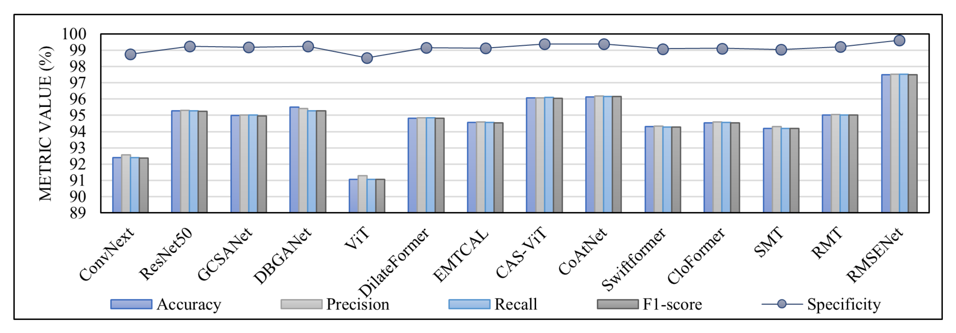
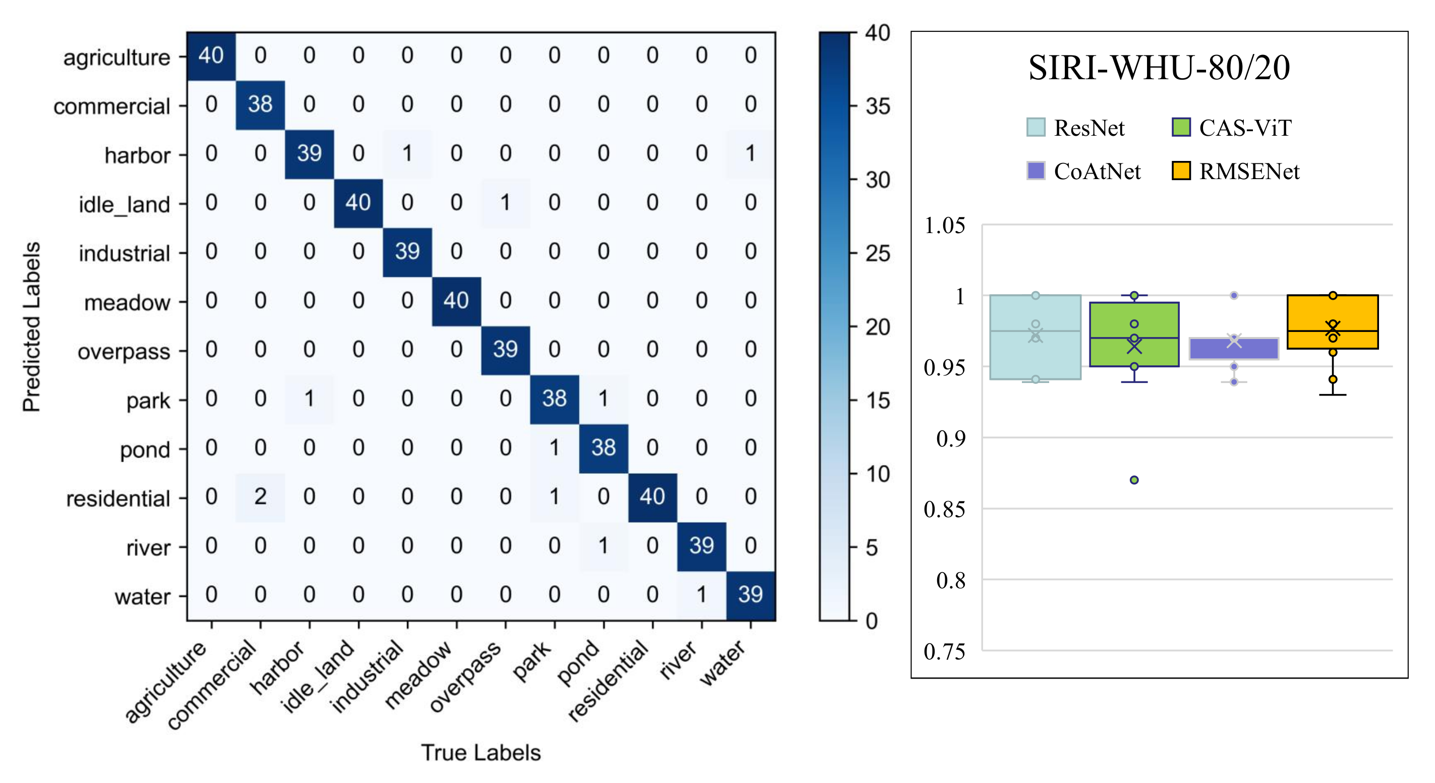
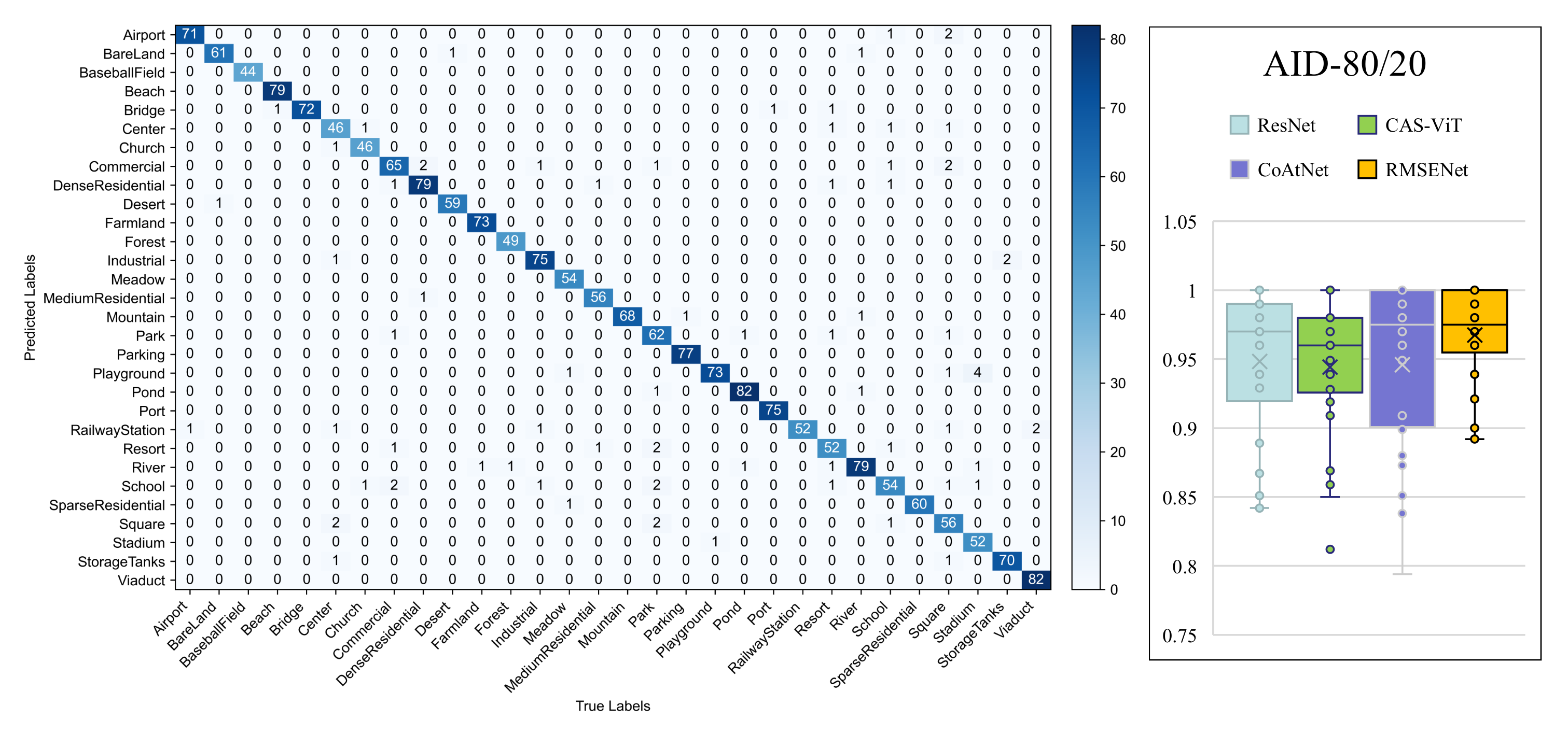
4.4. Comparative Experiments

In this paper, the average values of three experiments are adopted as the final experimental results, and three categories of high-performance models were selected as comparative models. The first category includes four CNN-based architectures, namely ConvNext [32], ResNet50, GCSANet [33], and DBGANet [34], which all utilize convolution for feature extraction and achieve excellent image classification performance through novel architectural designs. The second category consists of four Transformer-based architectures, including ViT, DilateFormer [35], EMTCAL [36], and CAS-ViT, which leverage self-attention mechanisms to capture global information and excel at processing high-resolution images. The third category consists of five hybrid CNN-Transformer architectures, such as CoAtNet, Swiftformer [37], CloFormer [38], SMT [39], and RMT [40], which combine the strengths of both CNNs and Transformers to extract complementary local and global features, thereby demonstrating superior representational capabilities for image data. By comparing RMSENet with these models of diverse architectures, this paper aims to illustrate the position and advantages of the proposed model within the broader model landscape and provide a comprehensive benchmark for future research. The comparison experimental results of RMSENet’s accuracy, precision, recall, specificity, and F1-score on the RSSCN7 dataset are shown in Figure 12. The number of parameters and calculation amount of each model are shown in

Table 1. Parameters and computational complexity of all networks involved in the comparison.

Model	Year	Params ($\times {10}^6$)	Flops ($\times {10}^6$)
ConvNext [32]	2022	28.75	4.46
ResNet50 [8]	2016	23.52	4.13
GCSANet [33]	2022	12.84	3.43
DBGANet [34]	2023	108.38	13.212
ViT [12]	2020	85.66	16.86
DilateFormer [35]	2022	23.48	4.41
EMTCAL [36]	2022	27.30	4.23
CAS-ViT [18]	2024	20.74	3.59
CoAtNet [19]	2021	16.99	3.35
Swiftformer [37]	2023	11.29	1.60
CloFormer [38]	2023	11.88	2.13
SMT [39]	2023	10.99	2.4
RMT [40]	2024	13.19	2.32
RMSENet	Ours	13.26	3.47

. The comparative experimental results of accuracy on the RSSCN7, AID, and SIRI-WHU datasets are presented in

Table 2. Comparison results of various network performance on the RSSCN7 dataset.

Model	RSSCN7-Accuracy (%)	Train	Test	Input Size
ConvNext	92.40 ± 0.80	2240	560	400 × 400
ResNet50	95.26 ± 0.09	2240	560	400 × 400
GCSANet	94.99 ± 0.72	2240	560	400 × 400
DBGANet	95.50 ± 0.50	2240	560	400 × 400
ViT	91.07 ± 0.54	2240	560	400 × 400
DilateFormer	94.81 ± 0.71	2240	560	400 × 400
EMTCAL	94.55 ± 0.09	2240	560	400 × 400
CAS-ViT	95.80 ± 0.27	2240	560	400 × 400
CoAtNet	96.13 ± 0.12	2240	560	400 × 400
Swiftformer	94.29 ± 0.54	2240	560	400 × 400
CloFormer	94.54 ± 0.62	2240	560	400 × 400
SMT	95.12 ± 0.06	2240	560	400 × 400
RMT	95.00 ± 0.89	2240	560	400 × 400
RMSENet	97.41 ± 0.09	2240	560	400 × 400

,

Table 3. Comparison results of various network performance on the AID dataset.

Model	AID-Accuracy (%)	Train	Test	Input Size
ConvNext	91.78 ± 0.28	8000	2000	600 × 600
ResNet50	95.0 ± 0.25	8000	2000	600 × 600
GCSANet	94.63 ± 0.07	8000	2000	600 × 600
DBGANet	94.40 ± 0.50	8000	2000	600 × 600
ViT	79.95 ± 0.15	8000	2000	600 × 600
DilateFormer	93.98 ± 0.68	8000	2000	600 × 600
EMTCAL	94.10 ± 0.45	8000	2000	600 × 600
CAS-ViT	94.0 ± 0.20	8000	2000	600 × 600
CoAtNet	94.82 ± 0.18	8000	2000	600 × 600
Swiftformer	93.10 ± 0.10	8000	2000	600 × 600
CloFormer	94.08 ± 0.18	8000	2000	600 × 600
SMT	93.43 ± 0.42	8000	2000	600 × 600
RMT	94.67 ± 0.23	8000	2000	600 × 600
RMSENet	95.9 ± 0.18	8000	2000	600 × 600

and

Table 4. Comparison results of various network performance on the SIRI-WHU dataset.

Model	SIRI-WHU-Accuracy (%)	Train	Test	Input Size
ConvNext	93.75 ± 0.41	1920	480	200 × 200
ResNet50	96.04 ± 0.21	1920	480	200 × 200
GCSANet	96.35 ± 0.32	1920	480	200 × 200
DBGANet	95.94 ± 0.52	1920	480	200 × 200
ViT	91.88 ± 0.21	1920	480	200 × 200
DilateFormer	95.96 ± 0.17	1920	480	200 × 200
EMTCAL	95.31 ± 0.52	1920	480	200 × 200
CAS-ViT	96.56 ± 0.52	1920	480	200 × 200
CoAtNet	96.41 ± 0.21	1920	480	200 × 200
Swiftformer	94.90 ± 0.52	1920	480	200 × 200
CloFormer	95.27 ± 0.36	1920	480	200 × 200
SMT	93.61 ± 0.14	1920	480	200 × 200
RMT	95.69 ± 0.14	1920	480	200 × 200
RMSENet	97.61 ± 0.21	1920	480	200 × 200

, respectively. Among them, the learning rate of ViT is set to 0.0001 due to overfitting. Compared to other models, RMSENet achieves the highest accuracy on the three datasets, with lower parameter and computation counts. Specifically, RMSENet improves accuracy by 2.15%, 0.9% and 1.57% compared to the classic CNN architecture model ResNet50 on the RSSCN7, AID and SIRI-WHU datasets, respectively, while also having lower parameter and computation counts. ViT excels at extracting global information but overlooks some detailed information, leading to the classification performance is not ideal. RMSENet outperforms the classic Transformer architecture model ViT on all three datasets. CoAtNet, as a classic hybrid architecture model, uses convolutional modules in the first two stages to extract local information and leverages a Transformer model in the last two stages to model long-range dependencies for extracting global information. Results from the three public datasets show that, with similar model complexity, RMSENet improves accuracy by 1.28%, 1.08% and 1.2% compared to CoAtNet.

The confusion matrix provides a more detailed view of the classification performance for each category, helping to understand which categories the model excels in and facilitating the analysis of the model. The boxplot [41] is a statistical chart that expresses data dispersion and is robust against outliers, offering a robust description of data dispersion, skewness, and tail weight. This paper employs boxplots based on the data on the main diagonal of the confusion matrix. RMSENet generates the confusion matrix on the RSSCN7 dataset, and the boxplot of each model based on the data on the main diagonal of the confusion matrix is shown in Figure 13. All 80 remote sensing images of the forest category were classified correctly, and of the 480 images from other categories, 466 were correctly classified, with only 14 images being misclassified. This indicates that RMSENet is most proficient in recognizing the forest category in the RSSCN7 dataset, and its performance in recognizing other categories is also relatively ideal, with no obvious difficulties in recognizing any remote sensing image categories. It can be seen from the comparison of the boxplot of each model that there are no abnormal values in the other three models, except ResNet, and RMSENet is superior to the other three models in terms of data concentration and skewness.

RMSENet generates the confusion matrix on the SIRI-WHU dataset, and the boxplot of each model based on the data on the main diagonal of the confusion matrix is shown in Figure 14. All remote sensing images in the three categories of agricultural areas, idle land, meadow and residential areas were correctly classified. Of the remaining 320 images, 309 were correctly classified, with only 11 images being misclassified. There were no categories with poor classification performance, indicating that RMSENet achieves ideal recognition results for all categories in the SIRI-WHU dataset. It can be seen from the comparison of the boxplot of each model that CAS-ViT and CoAtNet have outliers that are below the lower limit and above the upper limit, respectively, while RMSENet and ResNet have no outliers. Compared to ResNet, RMSENet exhibits better concentration and stability in the classification accuracy of various image categories.

RMSENet generates the confusion matrix on the AID dataset, and the boxplot of each model based on the data on the main diagonal of the confusion matrix is shown in Figure 15. There are 7 categories including 493 remote sensing images that are correctly classified, and there are no categories with a significantly poor classification effect. The smallest box height of RMSENet compared to the other three models reflects the smallest fluctuation in the accuracy for the classification of various scene images. It is demonstrated that the dispersion of classification accuracy for various scene images by RMSENet is small, and its stability is strong. It can basically accurately identify various categories in the dataset.

4.5. Visual Analysis

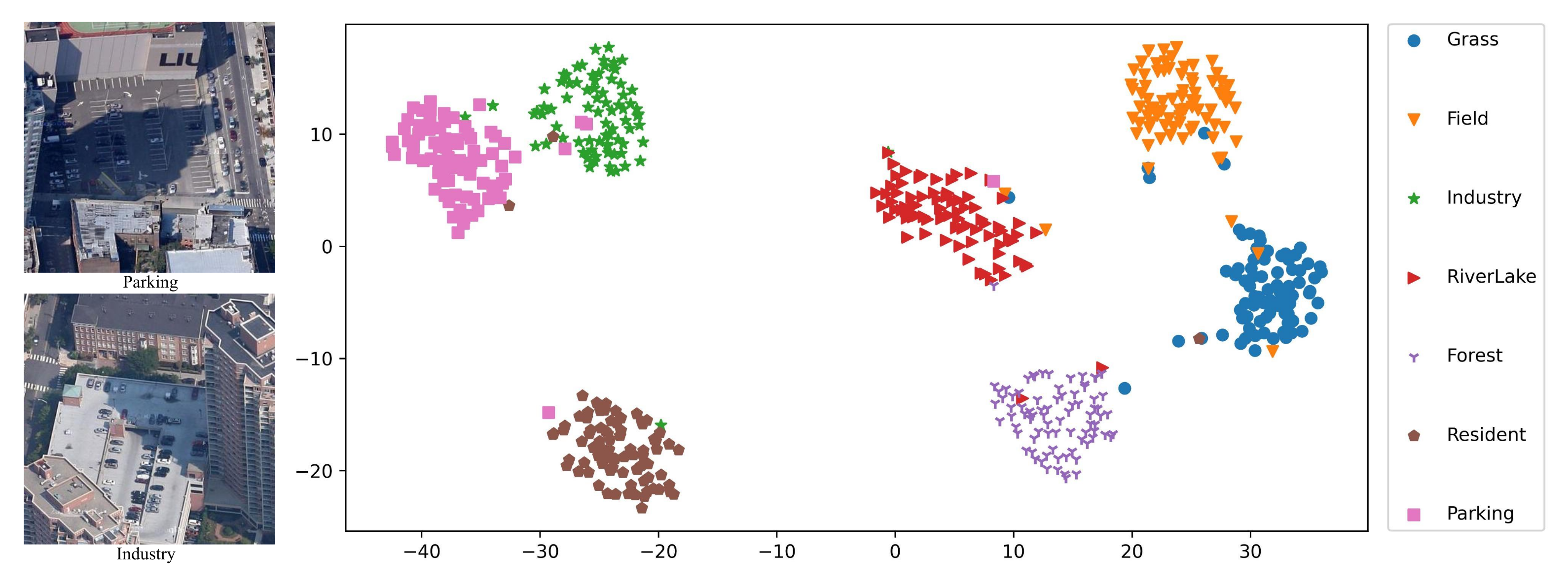
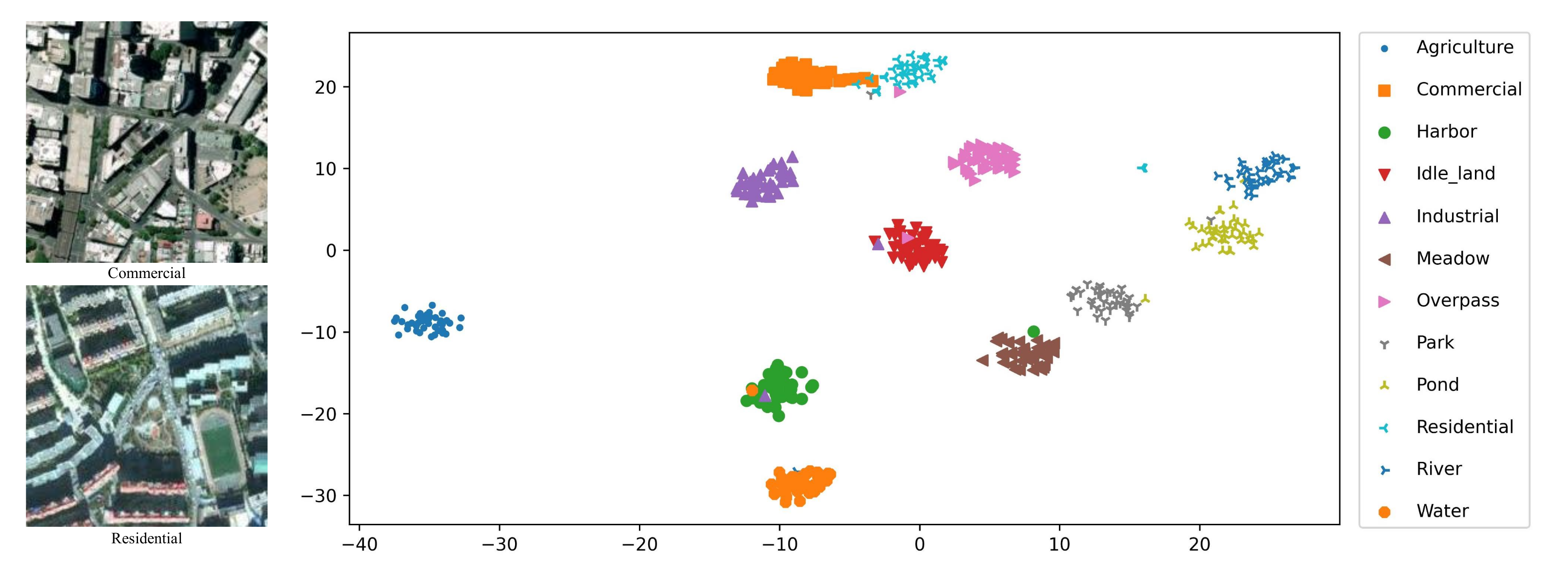
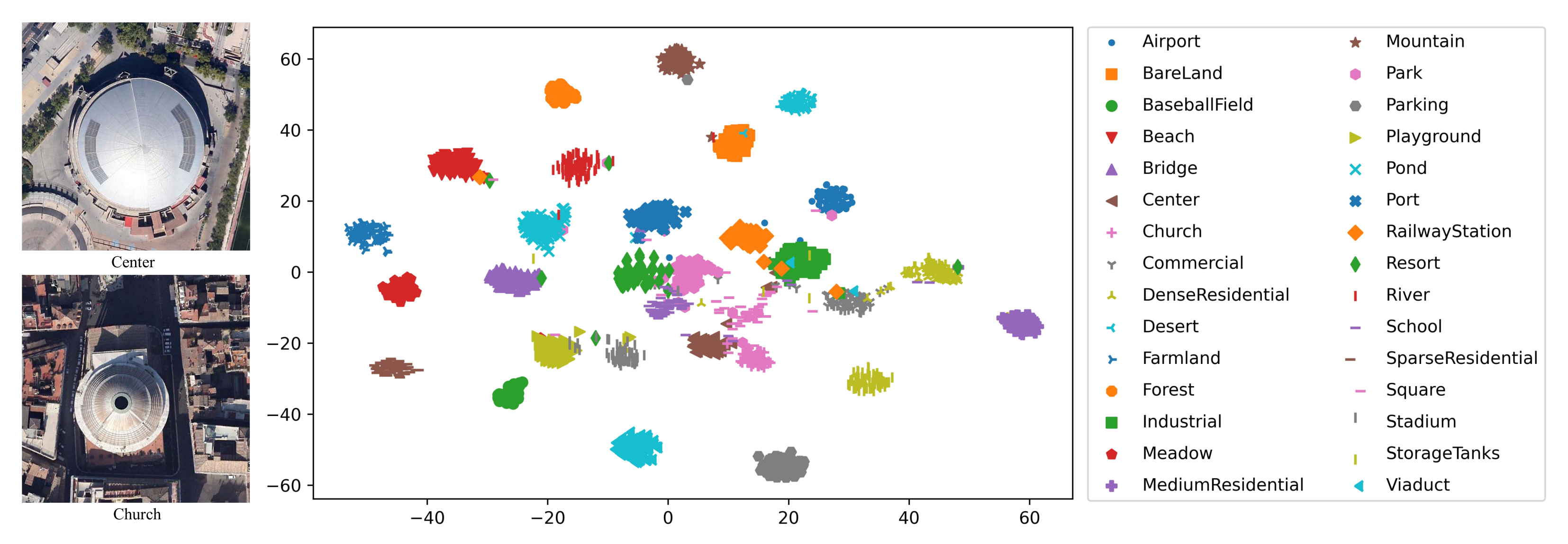
4.5.1. Visualization Analysis with t-SNE

To comprehensively evaluate the performance of RMSENet, this paper utilizes t-SNE [42] for visualization and analysis of dimensionality reduction data. t-SNE can map high-dimensional datasets to two- or three-dimensional spaces, preserving the local structure between data points, making similar samples closer together in the low-dimensional space and more distant from samples with larger differences. As shown in Figure 16, in the RSSCN7 dataset, factory scene images often contain parked vehicles, while parking lot scenes frequently include building structures resembling factories. Consequently, these two categories exhibit high inter-class visual similarity. The t-SNE visualization results generated by RMSENet on the RSSCN7 dataset further demonstrate that factory and parking lot sample points are closely clustered in the embedding space. Despite their pronounced inter-class similarity, samples from each category form relatively distinct clusters in the visualization, with only minor overlaps observed between a small subset of samples. This indicates that RMSENet performs effectively in addressing high inter-class similarity challenges within the RSSCN7 dataset.

As shown in Figure 17, in the SIRI-WHU dataset, both commercial and residential area scene categories are primarily characterized by dense building structures, resulting in high visual similarity between them. Although factory and parking lot samples project closely to each other in the low-dimensional embedding space, they maintain clear inter-cluster separation boundaries without significant overlap. These results demonstrate that RMSENet effectively mitigates feature confusion caused by high inter-class similarity in the SIRI-WHU dataset, validating the model’s robustness for complex scene classification tasks.

As shown in Figure 18, in the AID dataset, both central and church scene images exhibit prominent core architectural structures with similar shapes, resulting in high inter-class similarity. The t-SNE visualization generated by RMSENet on the AID dataset further confirms that the embeddings of central and church samples are closely projected in low-dimensional space. Despite their pronounced visual resemblance, the sample distributions of these two categories show no significant overlap or confusion in the t-SNE plot. This demonstrates RMSENet’s effectiveness in handling high inter-class similarity challenges within the AID dataset.

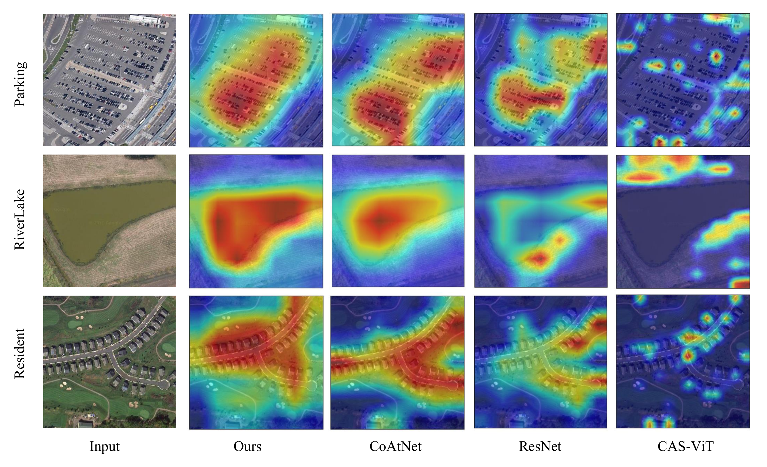
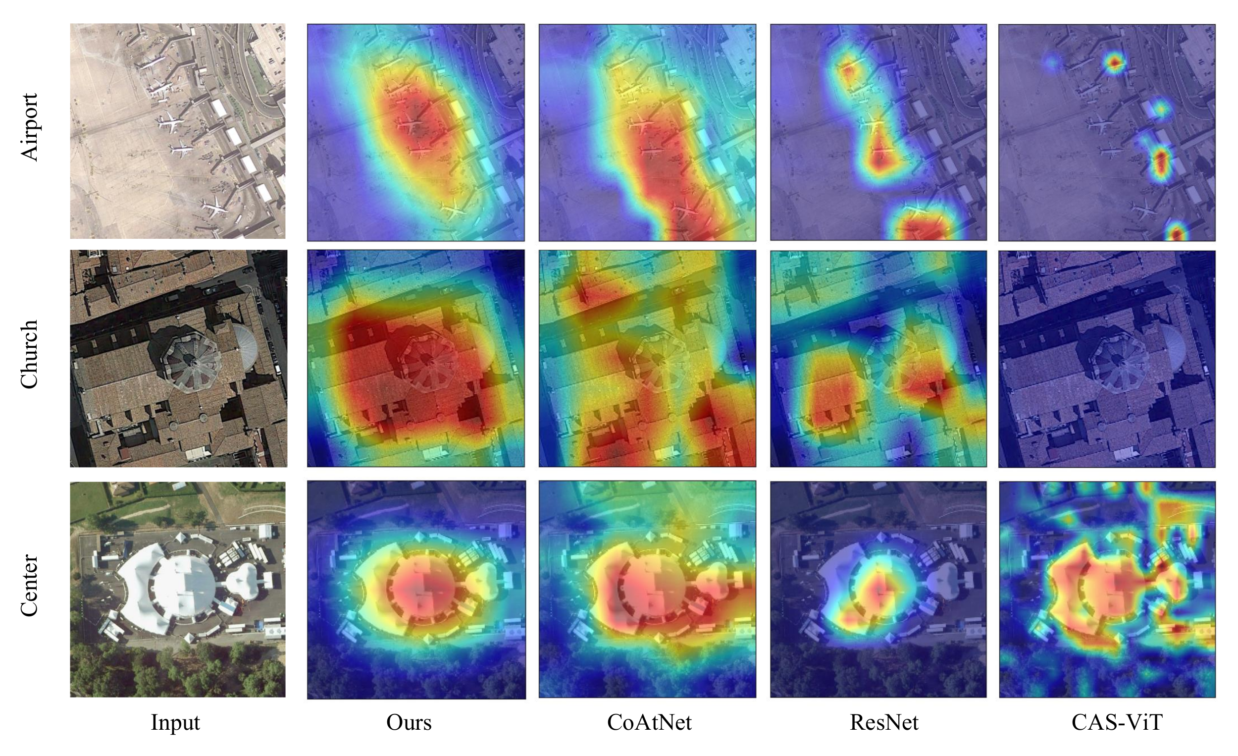
4.5.2. Visualization Analysis with Grad-CAM

This paper adopts Grad-CAM [43] to draw heatmaps and compares it with other models based on CNN architecture, Transformer architecture, and hybrid architecture to verify the effectiveness and classification performance of RMSENet. These heatmaps visualize the regions of interest for the model in the image. As the color changes from blue to red, the attention gradually focuses on more important areas. The heatmap comparison of RMSENet and other models on the RSSCN7, SIRI-WHU, and AID datasets is shown in Figure 19, Figure 20 and Figure 21. RMSENet can capture more pixel points conducive to target recognition compared to other models. For scenes with dense target objects, such as parking lots and residential areas, RMSENet can better capture the main features of the scene. For scenes with different image content, such as ports and riverlakes, the edge and contour information extracted by RMSENet are more obvious, closely focusing on the target objects. In summary, RMSENet can better grasp key information and identify scene images more accurately.

4.6. Ablation Experiments

This paper conducted ablation experiments on the RSSCN7 dataset from the perspectives of module splitting and module replacement to verify the role of each module in the model. “✓” and “×” were used in the experiments to indicate whether a module was utilized. The proposed multi-frequency coordinate channel attention (MFCA) and multi-scale wavelet self-attention (MWSA) modules in this paper are improvements over the current mainstream squeeze-and-excitation (SE) module and multi-head self-attention (MHSA), respectively. During the ablation experiments, the model used at most one MFCA and SE module; similarly, the model only used at most one of MWSA and MHSA. As shown in

Table 5. Effectiveness experiment of RMSENet modules on the RSSCN7 dataset.

Model	MFCA	SE	MWSA	MHSA	Slave-E	MFCF	Accuracy (%)
RMSENet	✓	×	✓	×	✓	✓	$97.41\pm 0.09$
RMSENet-1	✓	×	✓	×	×	✓	$96.60\pm 0.18$
RMSENet-2	✓	×	✓	×	✓	×	$96.87\pm 0.09$
RMSENet-3	×	×	✓	×	✓	✓	$96.18\pm 0.61$
RMSENet-4	×	✓	✓	×	✓	✓	$96.69\pm 0.03$
RMSENet-5	✓	×	×	✓	✓	✓	$96.60\pm 0.18$

, when the slave encoder in the model was removed (i.e., the proposed reverse cross-scale supplementation strategy was no longer adopted), the model’s accuracy significantly decreased, indicating that reversely supplementing the high-level semantic information extracted by the slave encoder to the shallow layers of the master encoder effectively enhances the feature extraction capability of the master encoder at all stages. When the multi-scale cross-fusion (MFCF) module in the model was removed (i.e., the proposed reverse cross-scale fusion strategy was no longer adopted), the model’s accuracy decreased, indicating that effectively fusing the features extracted by the last stage of the master encoder with those extracted by the first three stages can further utilize the local texture information extracted by the shallow network layers, helping the model make more correct decisions on the final scene classification results. When no channel attention mechanism was used in the model, the model’s accuracy significantly decreased, indicating that the interaction of channel information in feature maps is crucial. Additionally, when MFCA in the model was replaced with conventional SE, the accuracy of the model using SE was lower than that using MFCA, indicating that in MFCA, the spatial position information captured by global dependency modeling in two different directions (height and width) and the rich frequency information brought by discrete cosine transform (DCT) are valuable for fully extracting image features. Replacing MWSA with conventional MHSA caused a certain level of decrease in the model’s accuracy, indicating that MWSA’s feature extraction of remote sensing images from different scales and compensation for information loss caused by feature map downsampling through inverse wavelet transform operations play a positive role in enabling the model to more accurately recognize remote sensing images. When the proposed MWSA, MFCA, reverse cross-scale fusion strategy, and reverse cross-scale supplementation strategy worked synergistically, the model achieved the highest classification accuracy of 97.41% compared with the individual or partial combined effects of each module, and the experimental results were stable with a fluctuation of 0.09% across different batches. This indicates that MFCA (focused on capturing channel-wise interactions in feature maps) and MWSA (focused on extracting global features in the deep layers of the master encoder network), synergizing with the designed reverse cross-scale fusion strategy for the master encoder and the reverse cross-scale supplementation strategy for the slave encoder, enable the model to better extract features from remote sensing images and fully utilize the extracted features to determine the final scene classification results. In Table 5, Slave-E represents the slave encoder, and RMSENet denotes the model proposed in this paper.

As shown in

Table 6. Experimental results of wavelet transform basis function replacement for the RSSCN7 dataset.

Model	Wavelet Transform Basis Function	Accuracy (%)
RMSENet	Haar Wavelet	$97.41\pm 0.09$
RMSENet-6	Daubechies Wavelet	$96.78\pm 0.36$
RMSENet-7	Symlet Wavelet	$96.78\pm 0.36$
RMSENet-8	Coiflet Wavelet	$96.78\pm 0.36$
RMSENet-9	Biorthogonal Wavelet	$96.15\pm 0.26$
RMSENet-10	Reverse Biorthogonal Wavelet	$96.78\pm 0.18$

, using different wavelet transform basis functions has different effects on model recognition of remote sensing images. When Haar wavelet is chosen as the wavelet transform basis function, RMSENet performs best on the RSSCN7 dataset. Many remote sensing images have symmetry and repetition, such as residential areas and parking lots. Compared to other wavelet transform basis functions, the Haar wavelet has optimal symmetry [44], which is more sensitive to symmetric and repetitive remote sensing images and can more effectively capture local features of remote sensing images, improving the model’s recognition performance for remote sensing images. Additionally, the complexity of the Haar wavelet is the lowest compared to other wavelet basis functions, which helps avoid increased computational resource demands. Therefore, the wavelet transform basis function for the RMSENet model is chosen to be the Haar wavelet. The ablation experiments used each model three times to reduce the randomness of the experimental results.

5. Conclusions

This paper proposes a multi-scale reverse master–slave encoder network (RMSENet) for remote sensing image scene classification tasks. Experimental validation on three challenging open-source remote sensing image datasets (RSSCN7, SIRI-WHU, and AID) demonstrates RMSENet’s exceptional classification performance and the effectiveness of its proposed modules. Specifically, with lower parameter counts and computational requirements, RMSENet achieves classification accuracies of 97.41%, 95.9%, and 97.61% on the RSSCN7, AID, and SIRI-WHU datasets, respectively. Compared to the classic CNN architecture ResNet50, RMSENet shows improvements of 2.15%, 0.9%, and 1.57% on these datasets; against the Transformer-based CAS-ViT model, it achieves gains of 1.61%, 1.9%, and 1.05%. Moreover, it outperforms the hybrid architecture, CoAtNet, by 1.28%, 1.08%, and 1.2% in accuracy across the three datasets.

Future research will focus on two directions: first, on optimizing RMSENet’s architecture through transfer learning to further enhance classification performance, with comparative studies against other pre-trained remote sensing scene classification models; second, on conducting experiments using remote sensing image datasets with larger image dimensions and performing targeted model optimizations based on the experimental results to better meet practical application requirements.

References

1. Gong, J.; Zhang, M.; Hu, X.; Zhang, Z.; Li, Y.; Jiang, L. The design of deep learning framework and model for intelligent remote sensing. Acta Geod. Cartogr. Sin. 2022, 51, 475. [Google Scholar]
2. Quan, S.; Zhang, T.; Wang, W.; Kuang, G.; Wang, X.; Zeng, B. Exploring fine polarimetric decomposition technique for built-up area monitoring. IEEE Trans. Geosci. Remote Sens. 2023, 61, 5204719. [Google Scholar] [CrossRef]
3. Chen, L.; Li, S.; Bai, Q.; Yang, J.; Jiang, S.; Miao, Y. Review of image classification algorithms based on convolutional neural networks. Remote Sens. 2021, 13, 4712. [Google Scholar] [CrossRef]
4. Cha, Y.J.; Choi, W.; Büyüköztürk, O. Deep learning-based crack damage detection using convolutional neural networks. Comput. Aided Civ. Infrastruct. Eng. 2017, 32, 361–378. [Google Scholar] [CrossRef]
5. Cha, Y.J.; Ali, R.; Lewis, J.; Büyük, O. Deep learning-based structural health monitoring. Autom. Constr. 2024, 161, 105328. [Google Scholar] [CrossRef]
6. Vaswani, A.; Shazeer, N.; Parmar, N.; Uszkoreit, J.; Jones, L.; Gomez, A.N.; Kaiser, Ł.; Polosukhin, I. Attention is all you need. Adv. Neural Inf. Process. Syst. 2017, 30. [Google Scholar]
7. Kang, D.H.; Cha, Y.J. Efficient attention-based deep encoder and decoder for automatic crack segmentation. Struct. Health Monit. 2022, 21, 2190–2205. [Google Scholar] [CrossRef]
8. Ali, R.; Cha, Y.J. Attention-based generative adversarial network with internal damage segmentation using thermography. Autom. Constr. 2022, 141, 104412. [Google Scholar] [CrossRef]
9. Krizhevsky, A.; Sutskever, I.; Hinton, G.E. Imagenet classification with deep convolutional neural networks. Adv. Neural Inf. Process. Syst. 2012, 25, 84–90. [Google Scholar] [CrossRef]
10. He, K.; Zhang, X.; Ren, S.; Sun, J. Deep residual learning for image recognition. In Proceedings of the IEEE Conference on Computer Vision and Pattern Recognition, Las Vegas, NV, USA, 27–30 June 2016; pp. 770–778. [Google Scholar]
11. Tong, W.; Chen, W.; Han, W.; Li, X.; Wang, L. Channel-attention-based DenseNet network for remote sensing image scene classification. IEEE J. Sel. Top. Appl. Earth Obs. Remote Sens. 2020, 13, 4121–4132. [Google Scholar] [CrossRef]
12. Finder, S.E.; Amoyal, R.; Treister, E.; Freifeld, O. Wavelet convolutions for large receptive fields. In European Conference on Computer Vision; Springer Nature: Cham, Switzerland, 2024; pp. 363–380. [Google Scholar]
13. Cheng, X.; Li, B.; Deng, Y.; Tang, J.; Shi, Y.; Zhao, J. MMDL-Net: Multi-Band Multi-Label Remote Sensing Image Classification Model. Appl. Sci. 2024, 14, 2226. [Google Scholar] [CrossRef]
14. Dosovitskiy, A.; Beyer, L.; Kolesnikov, A.; Weissenborn, D.; Zhai, X.; Unterthiner, T.; Dehghani, M.; Minderer, M.; Heigold, G.; Gelly, S.; et al. An image is worth 16 × 16 words: Transformers for image recognition at scale. arXiv 2020, arXiv:2010.11929. [Google Scholar]
15. Liu, Z.; Lin, Y.; Cao, Y.; Hu, H.; Wei, Y.; Zhang, Z.; Lin, S.; Guo, B. Swin transformer: Hierarchical vision transformer using shifted windows. In Proceedings of the IEEE/CVF International Conference on Computer Vision, Montreal, BC, Canada, 11–17 October 2021; pp. 10012–10022. [Google Scholar]
16. Lv, P.; Wu, W.; Zhong, Y.; Du, F.; Zhang, L. SCViT: A spatial-channel feature preserving vision transformer for remote sensing image scene classification. IEEE Trans. Geosci. Remote Sens. 2022, 60, 4409512. [Google Scholar] [CrossRef]
17. Wu, N.; Lv, J.; Jin, W. S4Former: A Spectral–Spatial Sparse Selection Transformer for Multispectral Remote Sensing Scene Classification. IEEE Geosci. Remote Sens. Lett. 2024, 21, 5001605. [Google Scholar] [CrossRef]
18. Zhang, T.; Li, L.; Zhou, Y.; Liu, W.; Qian, C.; Hwang, J.-N.; Ji, X. Cas-vit: Convolutional additive self-attention vision transformers for efficient mobile applications. arXiv 2024, arXiv:2408.03703. [Google Scholar]
19. Dai, Z.; Liu, H.; Le, Q.V.; Tan, M. Coatnet: Marrying convolution and attention for all data sizes. Adv. Neural Inf. Process. Syst. 2021, 34, 3965–3977. [Google Scholar]
20. Xu, R.; Dong, X.-M.; Li, W.; Peng, J.; Sun, W.; Xu, Y. DBCTNet: Double branch convolution-transformer network for hyperspectral image classification. IEEE Trans. Geosci. Remote Sens. 2024, 62, 5509915. [Google Scholar] [CrossRef]
21. Zheng, Y.; Liu, S.; Chen, H.; Bruzzone, L. Hybrid FusionNet: A hybrid feature fusion framework for multisource high-resolution remote sensing image classification. IEEE Trans. Geosci. Remote Sens. 2024, 62, 5401714. [Google Scholar] [CrossRef]
22. Simonyan, K.; Zisserman, A. Very deep convolutional networks for large-scale image recognition. arXiv 2014, arXiv:1409.1556. [Google Scholar]
23. Deng, P.; Xu, K.; Huang, H. When CNNs meet vision transformer: A joint framework for remote sensing scene classification. IEEE Geosci. Remote Sens. Lett. 2021, 19, 8020305. [Google Scholar] [CrossRef]
24. Yang, Y.; Jiao, L.; Li, L.; Liu, X.; Liu, F.; Chen, P.; Yang, S. LGLFormer: Local–global lifting transformer for remote sensing scene parsing. IEEE Trans. Geosci. Remote Sens. 2023, 62, 5602513. [Google Scholar] [CrossRef]
25. Yue, H.; Qing, L.; Zhang, Z.; Wang, Z.; Guo, L.; Peng, Y. MSE-Net: A novel master–slave encoding network for remote sensing scene classification. Eng. Appl. Artif. Intell. 2024, 132, 107909. [Google Scholar] [CrossRef]
26. Yu, W.; Luo, M.; Zhou, P.; Si, C.; Zhou, Y.; Wang, X.; Feng, J.; Yan, S. Metaformer is actually what you need for vision. In Proceedings of the IEEE/CVF Conference on Computer Vision and Pattern Recognition, New Orleans, LA, USA, 18–24 June 2022; pp. 10819–10829. [Google Scholar]
27. Liu, L.; Liu, J.; Yuan, S.; Slabaugh, G.; Leonardis, A.; Zhou, W.; Tian, Q. Wavelet-based dual-branch network for image demoiréing. In Proceedings of the Computer Vision—ECCV 2020: 16th European Conference; Glasgow, UK, 23–28 August 2020, Proceedings, Part XIII 16; Springer International Publishing: Berlin/Heidelberg, Germany, 2020; pp. 86–102. [Google Scholar]
28. Zou, Q.; Ni, L.; Zhang, T.; Wang, Q. Deep learning based feature selection for remote sensing scene classification. IEEE Geosci. Remote Sens. Lett. 2015, 12, 2321–2325. [Google Scholar] [CrossRef]
29. Xia, G.-S.; Hu, J.; Hu, F.; Shi, B.; Bai, X.; Zhong, Y. AID: A benchmark data set for performance evaluation of aerial scene classification. IEEE Trans. Geosci. Remote Sens. 2017, 55, 3965–3981. [Google Scholar] [CrossRef]
30. Zhu, Q.; Zhong, Y.; Zhao, B.; Xia, G.-S.; Zhang, L. Bag-of-visual-words scene classifier with local and global features for high spatial resolution remote sensing imagery. IEEE Geosci. Remote Sens. Lett. 2016, 13, 747–751. [Google Scholar] [CrossRef]
31. Kingma, D.P.; Ba, J. Adam: A method for stochastic optimization. arXiv 2014, arXiv:1412.6980. [Google Scholar]
32. Liu, Z.; Mao, H.; Wu, C.-Y.; Feichtenhofer, C.; Darrell, T.; Xie, S. A convnet for the 2020s. In Proceedings of the IEEE/CVF Conference on Computer Vision and Pattern Recognition, New Orleans, LA, USA, 18–24 June 2022; pp. 11976–11986. [Google Scholar]
33. Chen, W.; Ouyang, S.; Tong, W.; Li, X.; Zheng, X.; Wang, L. GCSANet: A global context spatial attention deep learning network for remote sensing scene classification. IEEE J. Sel. Top. Appl. Earth Obs. Remote Sens. 2022, 15, 1150–1162. [Google Scholar] [CrossRef]
34. Xia, J.; Zhou, Y.; Tan, L. DBGA-Net: Dual-branch global–local attention network for remote sensing scene classification. IEEE Geosci. Remote Sens. Lett. 2023, 20, 7502305. [Google Scholar] [CrossRef]
35. Jiao, J.; Tang, Y.-M.; Lin, K.-Y.; Gao, Y.; Ma, J.; Wang, Y.; Zheng, W.-S. Dilateformer: Multi-scale dilated transformer for visual recognition. IEEE Trans. Multimed. 2023, 25, 8906–8919. [Google Scholar] [CrossRef]
36. Tang, X.; Li, M.; Ma, J.; Zhang, X.; Liu, F.; Jiao, L. EMTCAL: Efficient multiscale transformer and cross-level attention learning for remote sensing scene classification. IEEE Trans. Geosci. Remote Sens. 2022, 60, 5626915. [Google Scholar] [CrossRef]
37. Shaker, A.; Maaz, M.; Rasheed, H.; Khan, S.; Yang, M.-H.; Khan, F.S. Swiftformer: Efficient additive attention for transformer-based real-time mobile vision applications. In Proceedings of the IEEE/CVF International Conference on Computer Vision, Paris, France, 1–6 October 2023; pp. 17425–17436. [Google Scholar]
38. Fan, Q.; Huang, H.; Guan, J.; He, R. Rethinking local perception in lightweight vision transformer. arXiv 2023, arXiv:2303.17803. [Google Scholar]
39. Lin, W.; Wu, Z.; Chen, J.; Huang, J.; Jin, L. Scale-aware modulation meet transformer. In Proceedings of the IEEE/CVF International Conference on Computer Vision, Paris, France, 1–6 October 2023; pp. 6015–6026. [Google Scholar]
40. Fan, Q.; Huang, H.; Chen, M.; Liu, H.; He, R. Rmt: Retentive networks meet vision transformers. In Proceedings of the IEEE/CVF Conference on Computer Vision and Pattern Recognition, Seattle, WA, USA, 16–22 June 2024; pp. 5641–5651. [Google Scholar]
41. McGill, R.; Tukey, J.W.; Larsen, W.A. Variations of box plots. Am. Stat. 1978, 32, 12–16. [Google Scholar] [CrossRef]
42. Van der Maaten, L.; Hinton, G. Visualizing data using t-SNE. J. Mach. Learn. Res. 2008, 9, 2579–2605. [Google Scholar]
43. Selvaraju, R.R.; Cogswell, M.; Das, A.; Vedantam, R.; Parikh, D.; Batra, D. Grad-cam: Visual explanations from deep networks via gradient-based localization. In Proceedings of the IEEE International Conference on Computer Vision, Venice, Italy, 22–29 October 2017; pp. 618–626. [Google Scholar]
44. Wang, W.; Yang, T.; Wang, X. From Spatial to Frequency Domain: A Pure Frequency Domain FDNet Model for the Classification of Remote Sensing Images. IEEE Trans. Geosci. Remote Sens. 2024, 62, 5636413. [Google Scholar] [CrossRef]
Figure 1. Overall architecture of RMSENet.
Electronics 14 02479 g001
Figure 2. Semantic information extraction (SIE) module.
Electronics 14 02479 g002
Figure 3. Cross-scale spatial attention coding.
Electronics 14 02479 g003
Figure 4. Cross-scale channel attention coding.
Electronics 14 02479 g004
Figure 5. Local information extraction (LIE) module.
Electronics 14 02479 g005
Figure 6. Multi-frequency coordinate attention (MFCA) module.
Electronics 14 02479 g006
Figure 7. Local and global information extraction (LGIE) module.
Electronics 14 02479 g007
Figure 8. Multi-scale wavelet self-attention (MWSA) module.
Electronics 14 02479 g008
Figure 9. Examples of the RSSCN7 dataset.
Electronics 14 02479 g009
Figure 10. Examples of the AID dataset.
Electronics 14 02479 g010
Figure 11. Examples of the SIRI-WHU dataset.
Electronics 14 02479 g011
Figure 12. Comparative experiments on the RSSCN7 dataset.
Electronics 14 02479 g012
Figure 13. The experimental results of confusion matrix of RMSENet on the RSSCN7 dataset and a comparison of the experimental results of each network’s boxplot.
Electronics 14 02479 g013
Figure 14. The experimental results of the confusion matrix of RMSENet on the SIRI-WHU dataset and a comparison of the experimental results of each network’s boxplot.
Electronics 14 02479 g014
Figure 15. The experimental results of the confusion matrix of RMSENet on the AID dataset and a comparison of the experimental results of each network’s boxplot.
Electronics 14 02479 g015
Figure 16. High-similarity scene image on the RSSCN7 dataset and t-SNE visualization experiment results of RMSENet on the RSSCN7 dataset.
Electronics 14 02479 g016
Figure 17. High-similarity scene image on the SIRI-WHU dataset and t-SNE visualization experiment results of RMSENet on the SIRI-WHU dataset.
Electronics 14 02479 g017
Figure 18. High-similarity scene image on the AID dataset and t-SNE visualization experiment results of RMSENet on the AID dataset.
Electronics 14 02479 g018
Figure 19. Heatmaps of RMSENet and some models on the RSSCN7 dataset.
Electronics 14 02479 g019
Figure 20. Heatmaps of RMSENet and some models on the SIRI-WHU dataset.
Electronics 14 02479 g020
Figure 21. Heatmaps of RMSENet and some models on the AID dataset.
Electronics 14 02479 g021