Generalized Maximum Delay Estimation for Enhanced Channel Estimation in IEEE 802.11p/OFDM Systems

Abstract

This paper proposes a generalized maximum access delay time (MADT) estimation method for orthogonal frequency division multiplexing (OFDM) systems operating over multipath fading channels. The proposed approach derives a novel log-likelihood ratio (LLR) formulation by exploiting the correlation characteristics introduced by the cyclic prefix (CP) in received OFDM symbols, thereby enabling the efficient approximation of the maximum likelihood (ML) MADT estimation. A key contribution of this study is represented by the unification and generalization of existing MADT estimation methods by explicitly formulating the bias term associated with the geometric mean. Within this framework, a previously reported scheme is shown to be a special case of the proposed method. The effectiveness of the proposed MADT estimator is evaluated in terms of correct and good detection probabilities, illustrating not only improved detection accuracy but also robustness across varying channel conditions, in comparison with existing methods. Furthermore, the estimator is applied to both noise-canceling channel estimation (NCCE) and time-domain least squares (TDLS) methods, and its practical effectiveness is verified in IEEE 802.11p/OFDM system scenarios relevant to vehicle-to-everything (V2X) communications. Simulation results confirm that when integrated with NCCE and TDLS, the proposed estimator closely approaches the performance bound of ideal MADT estimation.

1. Introduction

Cooperative intelligent transportation systems (C-ITSs) have emerged as pivotal components in the development of smart transportation infrastructures, enabling real-time communication between vehicles and roadside infrastructure to enhance road safety and traffic efficiency [1]. As part of this evolution, vehicle-to-everything (V2X) communication has gained significant attention, necessitating reliable wireless communication protocols capable of operating in highly dynamic vehicular environments. To address these requirements, the IEEE 802.11p standard was introduced, defining the medium access control (MAC) and physical layer specifications for wireless access in vehicular environments (WAVE) [2]. IEEE 802.11p is derived from the IEEE 802.11a standard, with a key adaptation that reduces the channel bandwidth from 20 MHz to 10 MHz in order to improve robustness against multipath fading and Doppler effects prevalent in high-speed vehicular scenarios [2]. However, this reduction in bandwidth results in a corresponding decrease in the number of pilot subcarriers (i.e., only four pilot subcarriers) available per orthogonal frequency division multiplexing (OFDM) symbol. This limited number of pilots poses a significant challenge in accurately estimating channel variations in the frequency domain, especially under rapidly changing wireless conditions. As a result, ensuring the reliable and timely dissemination of traffic information requires enhanced channel estimation methods tailored to the constraints of IEEE 802.11p.

Various channel estimation (CE) techniques have been investigated for IEEE 802.11p/ OFDM systems [3,4,5,6,7,8,9,10,11,12]. To enhance the performance of the construct data pilot (CDP)-based scheme proposed in [1], the authors in [9] and refs. [4,5] have introduced the time-domain reliability test and frequency-domain interpolation (TRFI) scheme, as well as modified TRFI schemes utilizing virtual subcarriers for channel estimation. While these methods demonstrate performance enhancements, they are accompanied by relatively high computational complexity and inherent performance limitations. In particular, the studies in [4,5] assume that the channel impulse response (CIR) length is either perfectly known or set to $N_g-1$, where $N_g$ denotes the length of the cyclic prefix (CP), when estimating the channel frequency response (CFR) of virtual subcarriers.

In OFDM systems, low-complexity CE techniques are typically categorized into frequency-domain and time-domain approaches. In time-domain methods, the least square (LS) channel estimates, obtained by using pilot symbols or training sequences, are first transformed into the time domain via the inverse discrete Fourier transform (IDFT). Linear estimation is then applied in the time domain to reduce noise or perform interpolation, and the result is transformed back into the frequency domain to yield the CFR. Accordingly, the method proposed in [5] can be classified as a time-domain approach. Moreover, most practical OFDM systems employ null subcarriers at the spectrum edges to form guard bands, which can cause channel energy leakage even in sample-spaced channels. Several methods have been proposed to mitigate this effect [10,11,12]. Unlike these leakage mitigation approaches, the methods in [4,5] estimate the CFRs of virtual subcarriers directly.

Recently, the authors in [13] introduced a noise-canceling channel estimation (NCCE) technique that leverages the estimated channel length obtained from the algorithms presented in [6,7]. The NCCE scheme is based on a structure that performs inverse fast Fourier transform (IFFT), nulling, and fast Fourier transform (FFT) without relying on any interpolation techniques. However, its performance is highly sensitive to the accuracy of the channel length estimation, particularly in highly frequency-selective fading environments with long delay spreads.

The main contributions of this paper are summarized as follows:

1.

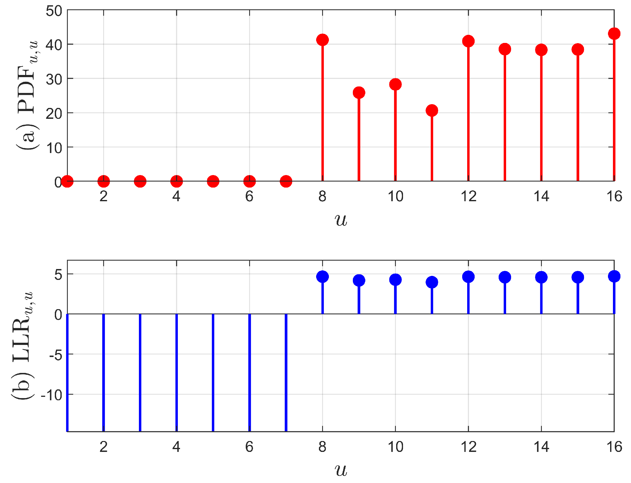
A novel log-likelihood ratio (LLR) expression is derived by exploiting the inherent correlation characteristics introduced by the cyclic prefix (CP) in the received OFDM symbols. This formulation enables the robust detection of the channel delay profile.

2.

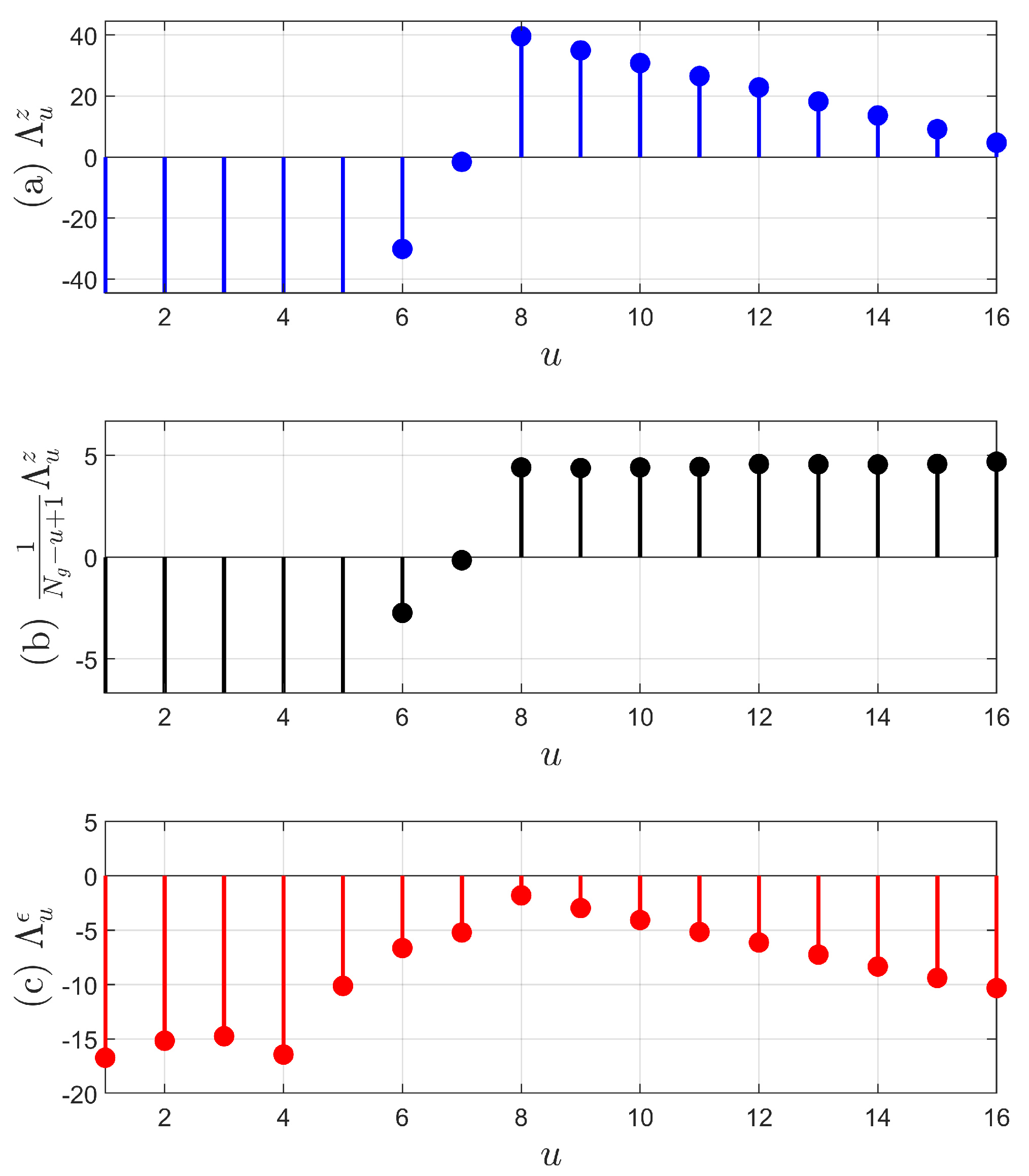
An approximated maximum likelihood (ML) estimator for the maximum access delay is proposed. The proposed estimator adopts a generalized form incorporating a weighting function applied to the observation random variables, thus enhancing detection accuracy under various channel conditions.

3.

The unification and generalization of existing methods are achieved by explicitly formulating the bias term associated with the geometric mean. It is analytically demonstrated that the estimator proposed in [6] represents a special case within the proposed framework, thereby extending and generalizing the prior approach.

4.

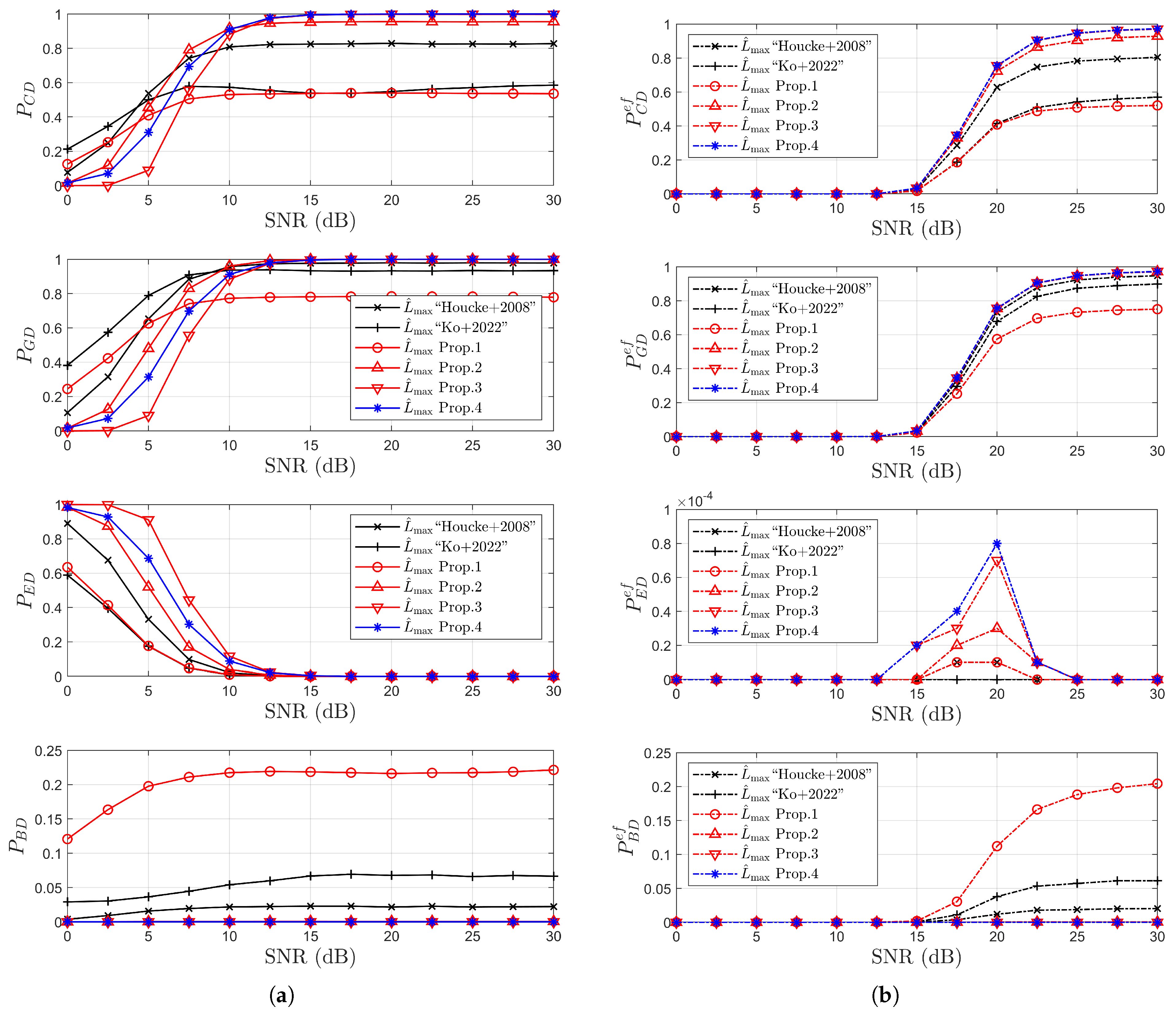
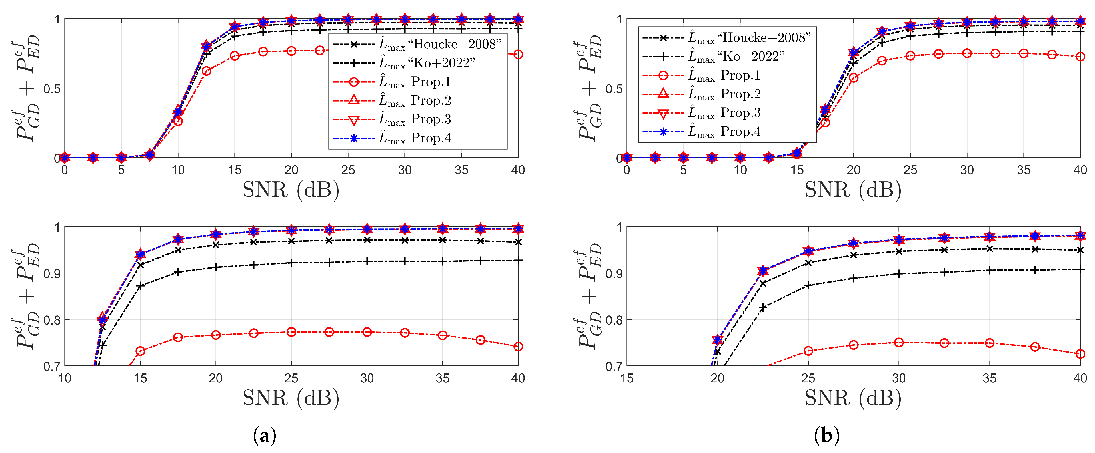
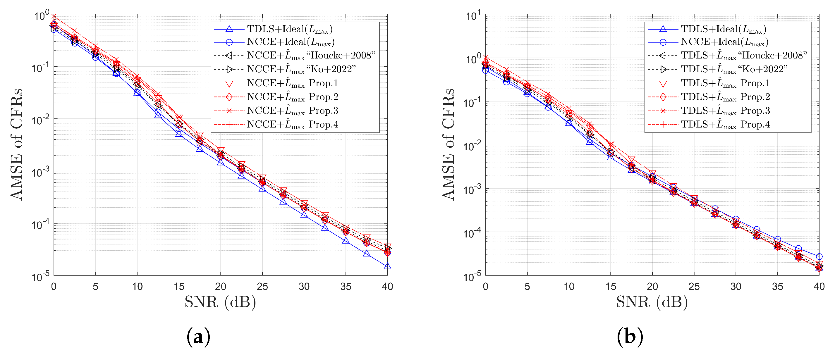
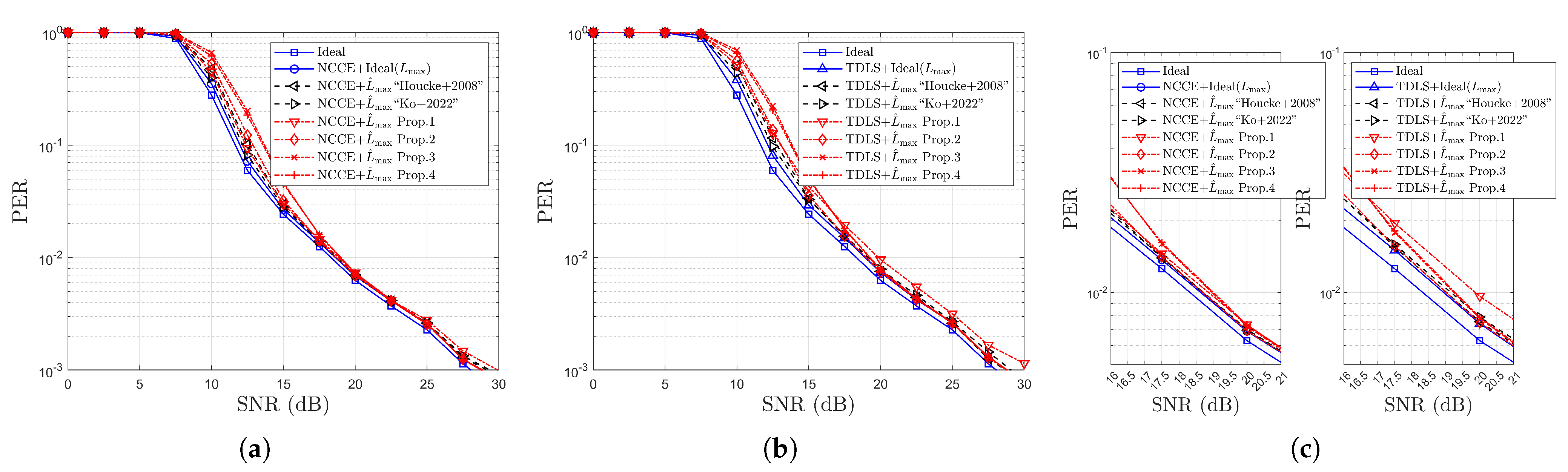
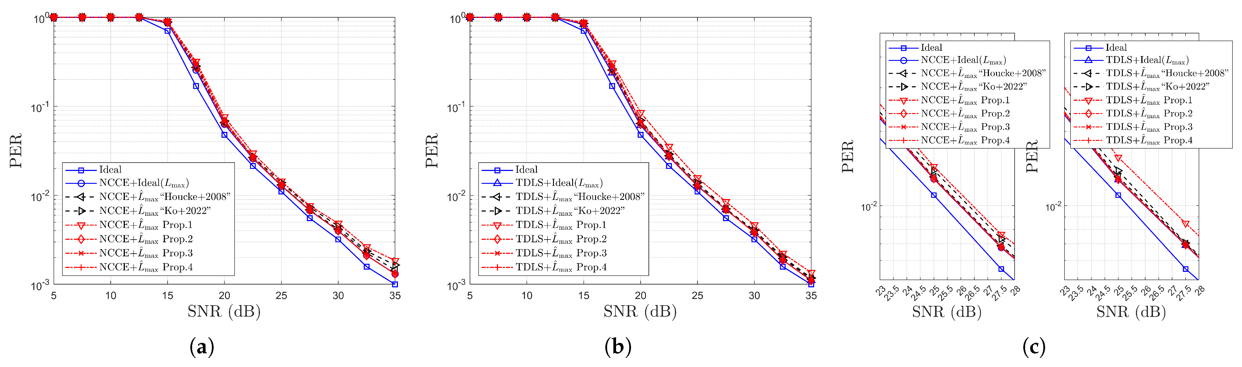
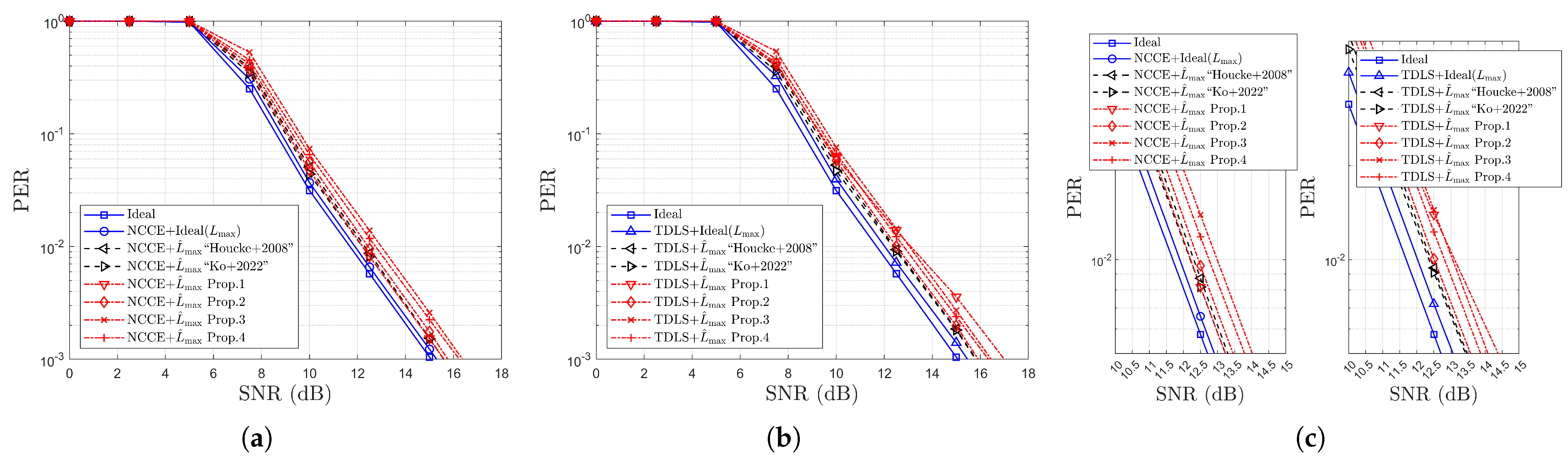
Performance advantages are demonstrated through extensive simulations, where the proposed scheme is applied to both the NCCE and the time-domain least square (TDLS) channel estimation methods. Simulation results under IEEE 802.11p/OFDM system conditions confirm the superiority of the proposed estimator in terms of correct and good detection probabilities. Notably, with respect to error rates, the proposed method closely approaches the performance bound of the ideal MADT estimation across all three considered channel environments.

Through these contributions, the proposed method not only improves the robustness of channel delay estimation but also enhances the overall performance of CE techniques in practical vehicular communication scenarios.

The remainder of this paper is organized as follows: Section 2 describes OFDM systems over multipath fading channels. The proposed channel delay estimation scheme is described in Section 3. Section 4 shows the simulation results, and concluding remarks are given in Section 5.

2. OFDM System and Discrete Signal Model

In OFDM systems, the source data are grouped and mapped onto modulated symbols $X_m\left(k\right)$, where $k\in \left\{0,1,\cdots ,N-1\right\}$, N is the IDFT size, and the symbols satisfy $E\left\{X_m\left(k\right)\right\}=0$ and $E\left\{{\left|X_m\left(k\right)\right|}^2\right\}=1$, with $E\left\{·\right\}$ denoting the expectation operator. The time-domain transmitted signal corresponding to the nth sample of the mth OFDM symbol is then obtained by applying the IDFT over N subcarriers and is given by

$$\begin{array}{cc}\hfill x_m\left(n\right)& ={\displaystyle \frac{1}{\sqrt{N}}}\sum _{k=0}^{N-1}{X}_m\left(k\right)e^{j2\pi kn/N},n=0,1,2,\cdots ,N-1\hfill \end{array}$$

(1)

where $E\left\{x_m\left(n\right)\right\}=0$ and $E\left\{{\left|x_m\left(n\right)\right|}^2\right\}=1$ [14,15,16].

To mitigate inter-symbol interference (ISI), a guard interval is appended to each OFDM symbol, comprising a CP that duplicates the last $N_g$ samples of the IDFT output. The length of the guard interval, $N_g$, is chosen to exceed the maximum delay spread of the channel. The transmitted signal propagates through a multipath fading channel, whose low-pass equivalent impulse response is given by

$$\begin{array}{c}\hfill h\left(t;\tau \right)=\sum _{l=0}^{L-1}{h}_l\left(t\right)\delta \left(\tau -{\tau }_l\right)\end{array}$$

(2)

where t, $\tau$, $\delta (·)$, L, and ${\tau }_l$ are the time, the delay, a Dirac delta function, the number of multipaths, and the propagation delay of the lth path, respectively [14]. The statistical characteristics of the multipath fading channel can be described by the wide-sense stationary uncorrelated scattering (WSSUS) model [15]. This model assumes that individual propagation paths are mutually uncorrelated and that the channel exhibits wide-sense stationarity in its correlation properties.

After removing the cyclic prefix, the discrete-time received signal can be expressed, from (1) and (2), as

$$\begin{array}{c}\hfill y_m\left(n\right)=\sum _{l=0}^{L-1}{h}_{l,m}\left(n\right)\sqrt{E_s}{x}_m\left({\left(n-d_l\right)}_N\right)+w_m\left(n\right)\end{array}$$

(3)

where $E_s$ is the transmitting signal power, ${(·)}_N$ represents a cyclic shift in the base of N, $w_m\left(n\right)\sim \mathcal{N}\left(0,{\sigma }^2\right)$ is complex additive white Gaussian noise (AWGN), $h_{l,m}\left(n\right)={\left.h_l\left(t\right)\right|}_{t=\left[m(N_g+N)+n\right]T_s}$ is the lth path channel gain of the nth sample for the mth OFDM symbol, and $d_l=\lfloor {\tau }_l/T_s\rfloor$ is the delay normalized by the sampling time $T_s$ [16]. For simplicity, we round $d_l$ to an integer without considering leakage. However, the correlation approach in this paper may also be extended to fractional $d_l$ [17]. When we assume the perfect synchronization as $d_l=l$ (i.e., ${\tau }_l=l{T}_s$) and the time-invariant channel within two consecutive OFDM symbols, the indexes m and $\left(n\right)$ in $h_{l,m}\left(n\right)$ of (3) can be omitted; then, we define $h_l$ as $h_l=\sqrt{E_s}{h}_{l,m}\left(n\right)$, where $E\left\{h_l\right\}=0$, $E\left\{{\left|h_l\right|}^2\right\}={\sigma }_l^2$, and ${\sigma }_h^2={\sum }_{l=0}^{L-1}{\sigma }_l^2=E_s$. The signal-to-noise ratio (SNR) can be written as $\mathrm{SNR}={\sigma }_h^2/{\sigma }^2=E_s/{\sigma }^2$. In addition, let us define the maximum number of paths including the zero channel gain path, from (3), as

$$\begin{array}{cc}\hfill L_{max}& =max\left\{d_l{|}_{l=0}^{L-1}\right\}+1\hfill \end{array}$$

(4)

where the maximum delay time, normalized by $T_s$, is $d_{max}=max\left\{d_l{|}_{l=0}^{L-1}\right\}=L_{max}-1$.

2.1. Joint PDFs

For $-N_g\le -k\le -1$$\left(\mathrm{i}.\mathrm{e}.,N_g\ge k\ge 1\right)$, the received signal samples at the border between two OFDM symbols can be written, from (3), as

$$\begin{array}{cc}\hfill y_m\left(-k\right)& =\sum _{l=0}^{L-1}{h}_l{x}_m\left(N-k-d_l\right)U\left(\left(N_g-k\right)-d_l\right)\hfill \\ \hfill & +\sum _{l=0}^{L-1}{h}_l{x}_{m-1}\left(N_s-k-d_l\right)U\left(\left(d_l-1\right)-\left(N_g-k\right)\right)+w_m(-k)\hfill \end{array}$$

(5)

where $N_s=N+N_g$ and $U\left(·\right)$ is the unit step function [17].

From (5), it is shown that the received signal has the ISI terms, related with $x_{m-1}\left(·\right)$, when $N_g\ge k\ge \left(N_g-d_{max}-1\right)$. Therefore, the correlation between each received signal over CP duration and its corresponding sample at the end of the OFDM symbol can be expressed as

$$\begin{array}{cc}\hfill & E\left\{y_m(-k)y_m^{*}(N-k)\right\}\hfill \\ \hfill & =\left\{\begin{array}{ccc}{\sigma }_h^2& \mathrm{if}\hfill & N_g-d_{max}\ge k\ge 1\\ \sum _{l=0}^{L-1}{\sigma }_l^{2}U\left(N_g-k-d_l\right)& \mathrm{else}\hfill & \left(N_g\ge k\ge N_g-d_{max}+1\right)\end{array}\right.\hfill \end{array}$$

(6)

where $k\in \left\{1,2,\cdots ,N_g\right\}$ [7,8,17,18]. Note that the expectation in (6) is taken with regard to the random variables of $\left\{h_l\right\}$, $\left\{x_m\left(n\right),x_{m-1}\left(n\right)\right\}$, and $\left\{w\left(n\right)\right\}$, which are assumed to be mutually independent for different indices l, m, and n.

When L is large, the signal ${\left.y_m\left(n\right)\right|}_{n=0}^{N-1-N_g}$ can be approximately modeled as a complex Gaussian random variable based on the central limit theorem [18,19]. The corresponding probability density function (PDF) is given from (6) as

$$\begin{array}{c}\hfill f\left(y_m\left(n\right)\right)={\displaystyle \frac{exp\left(-\frac{{\left|y_m\left(n\right)\right|}^2}{{\sigma }_h^2+{\sigma }^2}\right)}{\pi \left({\sigma }_h^2+{\sigma }^2\right)}}.\end{array}$$

(7)

For $k\in \left\{1,2,\cdots ,N_g\right\}$, the samples $y_m(-k)$ and $y_m(N-k)$ are jointly complex Gaussian. The joint PDF is given from (6) by

$$\begin{array}{c}\hfill f\left(y_m(-k),y_m(N-k)\right)={\displaystyle \frac{exp\left(-\frac{{\left|y_m(-k)\right|}^2+{\left|y_m(N-k)\right|}^2-2{\rho }_k\Re \left\{y_m(-k)y_m^{*}(N-k)\right\}}{\left({\sigma }_h^2+{\sigma }^2\right)\left(1-{\rho }_k^2\right)}\right)}{{\pi }^2\left({\sigma }_h^2+{\sigma }^2\right)\left(1-{\rho }_k^2\right)}}\end{array}$$

(8)

where $\Re \left\{·\right\}$ denotes the real part of a complex-valued input and ${\rho }_k$ represents the correlation coefficient between $y_m(-k)$ and $y_m(N-k)$. It yields

$$\begin{array}{cc}\hfill {\rho }_k& =\left|{\displaystyle \frac{E\left\{y_m(-k)y_m^{*}(N-k)\right\}}{\sqrt{E\left\{{\left|y_m(-k)\right|}^2\right\}E\left\{{\left|y_m(N-k)\right|}^2\right\}}}}\right|={\displaystyle \frac{{\sum }_{l=0}^{L-1}{\sigma }_l^{2}U\left(N_g-k-d_l\right)}{{\sigma }_h^2+{\sigma }^2}}.\hfill \end{array}$$

(9)

Note that $0<{\rho }_k<1$ and ${\rho }_{k+1}\le {\rho }_k$; i.e., ${\rho }_k$ is a non-increasing function with respect to k. Furthermore, we can find from (6) and (9) that the set ${\left\{{\rho }_k\right\}}_{k=1}^{N_g-d_{max}}$ consists of identical values, given by

$${\rho }_{N_g-d_{max}}=\cdots ={\rho }_2={\rho }_1={\displaystyle \frac{{\sigma }_h^2}{{\sigma }_h^2+{\sigma }^2}}.$$

2.2. N_g Noise Power Estimators

Assuming perfect synchronization at the receiver and a time-invariant channel over the duration of two consecutive OFDM symbols, $N_g$ noise variance estimators can be formulated from (5) and (6) as

$$\begin{array}{cc}\hfill {\widehat{\sigma }}^2& \leftarrow J\left(u\right),1\le u\le N_g\hfill \\ \hfill J\left(u\right)& ={\displaystyle \frac{1}{N_g-u+1}}\sum _{l=N_g}^{u}z\left(l\right)\hfill \end{array}$$

(10)

where

$$\begin{array}{cc}\hfill z\left(l\right)& ={\left.{\displaystyle \frac{1}{2M}}\sum _{m=1}^M{\left|y_m\left(-k\right)-y_m\left(N-k\right)\right|}^2\right|}_{k=N_g-l+1}\hfill \\ \hfill & ={\displaystyle \frac{1}{2M}}\sum _{m=1}^M{\left|y_m\left(-N_g+l-1\right)-y_m\left(N-N_g+l-1\right)\right|}^2\hfill \end{array}$$

(11)

and M denotes the number of OFDM symbols within the observation window (e.g., a packet or frame). It can be readily shown that the noise variance estimator achieves its minimum variance when $u=L_{max}\left(=d_{max}+1\right)$ [6,7,8].

For $L_{max}\le l\le N_g$, from (5), (6), and (9), $z\left(l\right)$ of (11) can be represented as

$$\begin{array}{cc}\hfill z\left(l\right){|}_{l=L_{max}}^{N_g}& ={\displaystyle \frac{1}{2M}}\sum _{m=1}^M{\left|y_m\left(-N_g+l-1\right)-y_m\left(N-N_g+l-1\right)\right|}^2\hfill \\ \hfill & ={\displaystyle \frac{1}{2M}}\sum _{m=1}^M{\left|w_m\left(-N_g+l-1\right)-w_m\left(N-N_g+l-1\right)\right|}^2\hfill \end{array}$$

(12)

where notice that $z\left(l\right)$ represents a random variable corresponding to the sum of exponentially distributed random variables. According to the central limit theorem (CLT) [19], for sufficiently large M, the distribution of $z\left(l\right)$ can be approximated by a Gaussian distribution as

$$\begin{array}{c}\hfill z\left(l\right){|}_{l=L_{max}}^{N_g}\sim \mathcal{N}\left({\sigma }^2,{\displaystyle \frac{{\sigma }^4}{M}}\right)\end{array}$$

(13)

where $E\left\{z\left(l\right){|}_{l=L_{max}}^{N_g}\right\}={\sigma }^2$ and $Var\left\{z\left(l\right){|}_{l=L_{max}}^{N_g}\right\}={\sigma }^4/M$.

It is important to note that for $1\le l<L_{max}$, $z\left(l\right)$ of (11) must be expressed in a form that includes ISI terms related with (6) and (9), rather than solely in terms of noise components, as in (12).

3. Proposed L_max Estimation Method in a Generalized Framework

From here, we propose the general method for $L_{max}$ estimation based on the observation variables of $\left\{z{\left(l\right)}_{l=u}^{N_g}\right\}$. When it is assumed that the given u is $L_{max}$ (i.e., $u\leftarrow L_{max}$), we can approximate ${\sigma }^2\simeq J\left(u\right)$; then, $f\left(\left.z\left(l\right)\right|u\leftarrow L_{max}\right)$ is computed, from (10) and (13), as

$$\begin{array}{cc}\hfill z\left(l\right){|}_{l=u,u\leftarrow L_{max}}^{N_g}& \sim \mathcal{N}\left(J\left(u\right),{\displaystyle \frac{J{\left(u\right)}^2}{M}}\right)\hfill \end{array}$$

(14)

and

$$\begin{array}{c}\hfill f_z\left(z\left(l\right)|u\leftarrow L_{max}\right){|}_{l=u}^{N_g}\approx {\displaystyle \frac{1}{\sqrt{2\pi J{\left(u\right)}^2/M}}}exp\left(-{\displaystyle \frac{{\left|z\left(l\right)-J\left(u\right)\right|}^2}{2J{\left(u\right)}^2/M}}\right).\end{array}$$

(15)

The LLR for (15) is written as

$$\begin{array}{cc}\hfill {\lambda }_{l|u}^z& =log\left(f_z\left(\left.z\left(l\right)\right|u\leftarrow L_{max}\right)\right)\hfill \\ \hfill & =-{\displaystyle \frac{{\left|z\left(l\right)-J\left(u\right)\right|}^2}{2J{\left(u\right)}^2/M}}-{\displaystyle \frac{log\left(2\pi J{\left(u\right)}^2/M\right)}{2}}.\hfill \end{array}$$

(16)

Figure 1 illustrates examples of the PDF $f_z\left(z\left(u\right)|u\leftarrow L_{max}\right)$, as defined in (15) with $l=u$, and the corresponding LLR ${\lambda }_{u|u}^z$ defined in (16) under the same condition, $l=u$. For $L_{max}\le u\le N_g$, the PDF value can exceed 1, as illustrated in Figure 1a, and the corresponding LLR is greater than 0, as depicted in Figure 1b. On the other hand, for $1\le u<L_{max}$, the PDF values are close to zero, and the corresponding LLRs are negative. Therefore, our goal is to identify the point, specifically $u=L_{max}$, at which the PDF value exhibits a sharp decline as u decreases from $N_g$ to 1. In order to present this concept in a generalized form, the random variable $ϵ\left(l\right)$ is defined as

$$\begin{array}{cc}\hfill ϵ\left(l\right)& ={\displaystyle \frac{1}{g\left(l\right)}}z\left(l\right)\hfill \end{array}$$

(17)

where $g\left(l\right)>0$ denotes a weighting function that transforms the random variable $z\left(l\right)$ into $ϵ\left(l\right)$. Furthermore, $g\left(l\right)$ is assumed to be a monotonically decreasing function with respect to the index l, such that the smallest value of u is estimated as $L_{max}$.

3.1. PDF Multiplication and Geometric Mean

Notice that $ϵ\left(l\right)$ can be approximated, for $L_{max}\le l\le N_g$ and large M, as the random variable of $ϵ\left(l\right)\sim \mathcal{N}\left({\displaystyle \frac{{\sigma }^2}{g\left(l\right)}},{\displaystyle \frac{{\sigma }^4}{Mg{\left(l\right)}^2}}\right)$ [6,8,19]. Since the different $z\left(l\right)$ are independent, the observation variables of $\left\{ϵ{\left(l\right)}_{l=u}^{N_g}\right\}$ are also mutually independent. Thus, ${\widehat{L}}_{max}$ can be obtained as the likelihood function of

$$\begin{array}{c}\hfill {\widehat{L}}_{max}=\arg \underset{1\le u\le N_g}{max}{\left[\prod _{l=N_g}^u{f}_{\mathbf{ϵ}}\left(\left.ϵ\left(l\right)\right|u\leftarrow L_{max}\right)\right]}^{1/(N_g-u+1)}\end{array}$$

(18)

where $f_{ϵ}\left(\left.ϵ\left(l\right)\right|u\leftarrow L_{max}\right)$ is computed from (15) and (17) with the approximation that ${\sigma }^2\simeq J\left(u\right)$. By assuming $L_{max}=u$ and considering the interval $u\le l\le N_g$, we can express

$$ϵ(l)\sim \mathcal{N}\left(\frac{J\left(u\right)}{g\left(l\right)},\frac{J{\left(u\right)}^2}{Mg{\left(l\right)}^2}\right)$$

(19)

and

$$\begin{array}{c}\hfill f_{\mathbf{ϵ}}\left(ϵ\left(l\right)|u\leftarrow L_{max}\right)=g\left(l\right)f_z\left(z\left(l\right)|u\leftarrow L_{max}\right).\end{array}$$

(20)

As discussed in [6], the expression in (18) represents an average likelihood function, where the likelihood is computed over a set of observation variables $\left\{ϵ\left(l\right){|}_{l=u}^{N_g}\right\}$ of (17). These variables are generally modeled as independent random variables, and their corresponding PDFs can vary in number depending on the delay spread or the estimated maximum channel length. Due to this variable-length observation set, the joint likelihood of the observations cannot be expressed by using a fixed-length product of PDFs. Instead, to ensure statistical consistency and comparability across different lengths, the geometric mean of the individual PDFs is used as in (18), which maintains the overall scale of the likelihood irrespective of the number of observations. This formulation preserves the multiplicative structure of independent observations while normalizing the outcome to allow for a meaningful comparison across different hypotheses or models with different numbers of taps. This approach reflects a fundamental principle in statistical signal processing, where the likelihood function must account for both the independence and variable dimensionality of the underlying random observations to remain statistically robust.

3.2. LLR Summation and Average

From (17) and (19), we can rewrite (18) as the LLR form of

$$\begin{array}{cc}\hfill {\Lambda }_u^{ϵ}={\Lambda }_u^{ϵ}\left(\left.{\left\{ϵ\left(l\right)\right\}}_{l=u}^{N_g}\right|u\leftarrow L_{max}\right)& =log{\left[\prod _{l=N_g}^u{f}_{ϵ}\left(\left.ϵ\left(l\right)\right|u\leftarrow L_{max}\right)\right]}^{1/(N_g-u+1)}\hfill \\ \hfill & ={\displaystyle \frac{1}{N_g-u+1}}\sum _{l=N_g}^{u}log\left(f_{ϵ}\left(\left.ϵ\left(l\right)\right|u\leftarrow L_{max}\right)\right)\hfill \end{array}$$

(21)

where $1\le u\le N_g$. From ${\lambda }_{l|u}^z$ of (16), it yields

$$\begin{array}{c}\hfill {\Lambda }_u^{ϵ}={\Lambda }_u^{ϵ}\left(\left.{\left\{ϵ\left(l\right)\right\}}_{l=u}^{N_g}\right|u\leftarrow L_{max}\right)={\displaystyle \frac{{\Lambda }_u^z}{N_g-u+1}}+B_u\end{array}$$

(22)

where

$$\begin{array}{cc}\hfill {\Lambda }_u^z& ={\Lambda }_u^z\left(\left.{\left\{z\left(l\right)\right\}}_{l=u}^{N_g}\right|u\leftarrow L_{max}\right)=\sum _{l=N_g}^u{\lambda }_{l|u}^z\hfill \\ \hfill & =-\sum _{l=N_g}^u{\displaystyle \frac{{\left|z\left(l\right)-J\left(u\right)\right|}^2}{2J{\left(u\right)}^2/M}}-\left(N_g-u+1\right){\displaystyle \frac{log\left(2\pi J{\left(u\right)}^2/M\right)}{2}}.\hfill \end{array}$$

(23)

and

$$B_u=\frac{1}{N_g-u+1}\sum _{l=N_g}^{u}log\left(g\left(l\right)\right).$$

(24)

Then, from (18) and (22), the maximum access delay time can be alternatively estimated as

$$\begin{array}{cc}\hfill {\widehat{L}}_{max}& =\arg \underset{1\le u\le N_g}{max}\left[{\Lambda }_u^{ϵ}\left(\left.{\left\{ϵ\left(l\right)\right\}}_{l=u}^{N_g}\right|u\leftarrow L_{max}\right)\right].\hfill \end{array}$$

(25)

Fundamentally, the CIR length estimator, expressed by (18) and (25), is based on the $N_g$ noise estimator $J\left(u\right)$ of (10). In (18) and (25), the given u (i.e., $u\leftarrow L_{max}$) indicates that $z\left(l\right){|}_{l=u}^{N_g}$ of (12) can be each noise estimator. Accordingly, $J\left(u\right)$ among $\left\{J\left(l\right){|}_{l=u}^{N_g}\right\}$ can be regarded as the estimator with the smallest variance. Therefore, as confirmed in (19), not $J\left(l\right)$ but $J\left(u\right)$ can be utilized.

3.3. Special Cases for $g\left(l\right)$

To illustrate the impact of the function $g\left(l\right)$ in the proposed scheme, the $L_{max}$ estimation method presented in [6] is first considered.

3.3.1. Method in [6] with $g\left(l\right)=\left(N_g-l+1\right)$

From (10) and (11), the uth noise variance estimator of $J\left(u\right)$ can be represented with regard to $\left\{ϵ\left(l\right)\right\}$ as

$$J\left(u\right)=\frac{1}{N_g-u+1}\frac{N_g-u}{1}J(u+1)+ϵ\left(u\right)$$

(26)

and

$$\begin{array}{cc}\hfill ϵ\left(l\right)& ={\displaystyle \frac{1}{N_g-l+1}}z\left(l\right).\hfill \end{array}$$

(27)

Note that the estimator described in [6] uses $g\left(l\right)=\left(N_g-l+1\right)$ obtained from (26). From (22) and (24), the LLR summation is expressed as a function of $z\left(l\right){|}_{l=u}^{N_g}$ and has the bias term of

$$\begin{array}{c}\hfill B_u={\displaystyle \frac{log\left[\left(N_g-u+1\right)!\right]}{\left(N_g-u+1\right)}}.\end{array}$$

(28)

As a result, the bias term involving $log\left[\left(N_g-u+1\right)!\right]$ is attributed to the structure of $g\left(l\right)=\left(N_g-l+1\right)$, while the corresponding geometric mean produces a scaling factor of $1/\left(N_g-u+1\right)$.

The operation of the proposed method, as formulated in (18) and (25), is described as follows: Figure 1 shows the examples for $f_z{\left(z\left(l\right)|u\leftarrow L_{max}\right)}_{l=u}$ of (15) and ${\left({\lambda }_{l|u}^z\right)}_{l=u}$ of (16). Examples of ${\Lambda }_u^z$, ${\displaystyle \frac{1}{N_g-u+1}}{\Lambda }_u^z$, and ${\Lambda }_u^{ϵ}$, as defined in (22), (23), and (22) with (28), are depicted in Figure 2 for cases (a), (b), and (c), respectively.

For $L_{max}\le u\le N_g$, the values of $\left\{f_z\left(z\left(l\right)\right){|}_{l=N_g}^u\right\}$ are observed to be similar, as shown in Figure 1a. Accordingly, the values of $\left\{f_{ϵ}\left(ϵ\left(l\right)\right){|}_{l=N_g}^u\right\}$ in (20) increase as l decreases from $N_g$ to u, due to the scaling effect of $g\left(l\right)=\left(N_g-l+1\right)$. As a result, the method proposed in [6], utilizing $\left\{ϵ\left(l\right)\right\}$ derived from $\left\{z\left(l\right)\right\}$, can be interpreted as a specific instance of the proposed approach, wherein the weight function $g\left(l\right)=\left(N_g-l+1\right)$ is employed. In (27), the weighting factors $\left\{1/\left(N_g-l+1\right)\right\}$ are chosen based on the relationship among $\left\{J\left(u\right)\right\}$. This mechanism leads to the bias term described in (22), which is further detailed in (28), resulting in an increase in the LLR summation as u decreases from $N_g$ to u, as illustrated in Figure 2c.

Figure 2a shows that ${\Lambda }_u^z$ of (23) increases as u decreases from $N_g$ to $L_{max}$. In this range, each decrement in u results in the multiplication of a PDF value greater than 1, as shown in Figure 1a, which corresponds to the addition of a positive LLR value in (23), as seen in Figure 1b. Conversely, when u is reduced from $d_{max}\left(=L_{max}-1\right)$ to 1, a PDF value less than 1, as shown in Figure 1a, is successively multiplied. This is equivalent to adding a negative LLR value in (23), as illustrated in Figure 1b, thereby causing a sharp decline in the LLR summation, as depicted in Figure 2a. For ${\displaystyle \frac{1}{N_g-u+1}}{\Lambda }_u^z$, Figure 2b shows a plateau starting at $u=L_{max}$. The width of this plateau is equal to $N_g-L_{max}+1$. Nevertheless, the method in [6], utilizing $\left\{ϵ\left(l\right)\right\}$ of (27), does not exhibit a plateau in the region $L_{max}\le u\le N_g$, as shown in Figure 2c. This behavior is attributed to the presence of the bias term described in (28). From Figure 2c, the estimated value ${\widehat{L}}_{max}=8$ is obtained by using the criterion in (25).

3.3.2. Proposed $g\left(l\right)$

In this paper, we propose the estimators utilizing $g\left(l\right)$ as follows:

• (Prop.1) $g\left(l\right)=\sqrt{N_g-l+1}$→$B_u={\displaystyle \frac{log\left[\left(N_g-u+1\right)!\right]}{2\left(N_g-u+1\right)}}$.
• (Prop.2) $g\left(l\right)={\left(N_g-l+1\right)}^2$→$B_u={\displaystyle \frac{2log\left[\left(N_g-u+1\right)!\right]}{\left(N_g-u+1\right)}}$.
• (Prop.3) $g\left(l\right)=e^{N_g-l}$→$B_u={\displaystyle \frac{N_g-u+1}{2}}$.
• (Prop.4) $g\left(l\right)={\left[f_z\left(z\left(l\right)|u\leftarrow L_{max}\right)\right]}^{N_g-u}$→$B_u={\displaystyle \frac{N_g-u}{N_g-u+1}}{\Lambda }_u^z$.

From the derived results, it can be concluded that the function $g\left(l\right)$, in (17) and (20), serves as a weighting factor for $z\left(l\right)$, enabling the identification of the endpoint of the plateau observed in Figure 2b. This mechanism can be interpreted such that as the estimation scheme evolves from ‘Prop.1’ to ‘Prop.3’ (including the case where $g\left(l\right)=\left(N_g-l+1\right)$ in [6]), the proposed estimator employs a progressively increasing weight for smaller values of u. This strategy facilitates the selection of the smallest possible u as the estimate ${\widehat{L}}_{max}$. A detailed performance comparison among these schemes is provided in Section 4.

For a special case, let us consider ‘Prop.4’, under which (21) can be reformulated as follows:

$${\Lambda }_u^{ϵ}=\sum _{l=N_g}^{u}log\left(f_z\left(\left.z\left(l\right)\right|u\leftarrow L_{max}\right)\right)=\sum _{l=N_g}^u{\lambda }_{l|u}^z={\Lambda }_u^z$$

(29)

Figure 2a presents the result corresponding to ‘Prop.4’. Although (29) does not appear to represent an average likelihood in the form of a geometric mean of the individual PDF elements, the proposed approach demonstrates that the weight function $g\left(u\right)$ is incorporated prior to averaging the LLR summation.

3.4. Computational Complexity

Table 1. Computational complexity comparison.

Term	1 Operation	Number
	$+/-$	$\left(8M+3N_g-1\right)N_g/2$
Prop.1 and 2, ${\widehat{L}}_{max}$ [6]	$\times /÷$	$\left(2M+N_g+6\right)N_g$
	log	$2N_g$
	$+/-$	$\left(8M+3N_g-1\right)N_g/2$
2 Prop.3 and 4	$\times /÷$	$\left(4M+N_g+15\right)N_g/2$
	log	$N_g$
	$+/-$	$\left(3N_g+N\right)M+\left(3N_g+13\right)N_g/2-3$
3 ${\widehat{L}}_{max}$ [7]	$\times /÷$	$\left(4M+4N_g+7\right)N_g+\left(2M+1\right)N$
	log	$N_g$

¹ Not complex but real operation. ² In Prop.3 and Prop.4 of (29), no numerical operations related to $B_u$ are required. ³ Additionally, it is necessary to determine the real roots of $N_g$ cubic equations [8].

compares the computational complexity of the proposed schemes with those of the existing methods presented in [6,7]. As shown in Table 1, for both the proposed schemes and the method in [6], the dominant term determining the complexity of the multiplication operations is a function of $2M{N}_g$. In contrast, the dominant term for the method in [7] is a function of $2MN$. Therefore, even when excluding the operations required to compute the real roots of $N_g$ cubic equations, the method in [7] exhibits the highest overall complexity. Meanwhile, the complexity of the proposed schemes is comparable to that of the method in [6].

4. Simulation Results

In this paper, a generalized $L_{max}$ estimation method is proposed and applied to OFDM channel estimation techniques, specifically to TDLS in [3] and NCCE in [13]. The performance of the proposed approach is evaluated through simulation. It is worth noting that NCCE can be implemented by using a sequence of IFFT/nulling/FFT operations, as shown in

Table 2. Legend description for simulation results.

Comments	Legend	${\widehat{\mathit{L}}}_{max}$	IFFT/Nulling/FFT
	Ideal
Bounds	$\mathtt{TDLS}+\mathtt{Ideal}\left(L_{max}\right)$	$L_{max}$	Not applicable
	$\mathtt{NCCE}+\mathtt{Ideal}\left(L_{max}\right)$	$L_{max}$	2 O
[3] + [6]	$\mathtt{TDLS}+{\widehat{L}}_{max}$ “Houcke+2008”	By (5) in [6]	Not applicable
[3] + [7]	$\mathtt{TDLS}+{\widehat{L}}_{max}$ “Ko+2022”	By (16) in [7]	Not applicable
[3] + $\mathrm{Prop}.{\mathrm{X}}^1$	$\mathtt{TDLS}+{\widehat{L}}_{max}\mathrm{Prop}.{\mathrm{X}}^1$	By (18) and (25)	Not applicable
[13] + [6]	$\mathtt{NCCE}+{\widehat{L}}_{max}$ “Houcke+2008”	By (5) in [6]	2 O
[13] + [7]	$\mathtt{NCCE}+{\widehat{L}}_{max}$ “Ko+2022”	By (16) in [7]	2 O
[13] + $\mathrm{Prop}.{\mathrm{X}}^1$	$\mathtt{NCCE}+{\widehat{L}}_{max}\mathrm{Prop}.{\mathrm{X}}^1$	By (18) and (25)	2 O

¹$X\in \left\{1,2,3,4\right\}$ in Section 3.3.2. ² NCCE can be implemented by using a sequence of IFFT/nulling/FFT operations [13].

, resulting in lower computational complexity compared with TDLS.

In this section, simulation results are presented to evaluate the detection probabilities, error rate, and MSE performance of the proposed scheme. The simulations are conducted based on the IEEE 802.11p standard with system parameters set to $N=64$, $N_g=16$, and $T_s=0.1\mathrm{\mu }$s [2,8]. Both the transmitter and receiver employ a convolutional encoder and a Viterbi decoder with a constraint length of 7 [2,8]. Each packet consists of $M\left(=100\right)$ OFDM symbols, with quadrature phase shift keying (QPSK) and 16-quadrature amplitude modulation (QAM) modulation schemes used at a coding rate of 1/2. All performance metrics are averaged over $5\times {10}^5$ packet transmissions to ensure statistical reliability. Additional simulation parameters are provided in Table 3 of [8]. Among five scenarios of ‘CohdaWireless V2V channel model’ in [20], we consider the ‘Highway NLOS with 252 km/h’, ‘Street Crossing NLOS with 126 km/h’, and ‘Highway LOS with 252 km/h’ channel environments, the channel profiles of which are presented in

Table 3. Channel profile due to scenarios in [20] (see Table 4 in [8]).

Ch. Type	Item	Tap 0	Tap 1	Tap 2	Tap 3	Unit
Highway	Power	0	$-2$	$-5$	$-7$	dB
NLOS	Delay$\left({\tau }_l\right)$	0	200	433	700	ns
$\left(252\mathrm{km}/\mathrm{h},\right.$	$d_l$	$d_0=0$	$d_2=2$	$d_4=4$, $d_5=5$	$d_7=7$	$\times T_s$
$\left.L_{max}=8\right)$	Doppler	0	689	$-492$	886	Hz
Street Crossing	Power	0	$-3$	$-5$	$-10$	dB
NLOS	Delay$\left({\tau }_l\right)$	0	267	400	533	ns
$\left(126\mathrm{km}/\mathrm{h},\right.$	$d_l$	$d_0=0$	$d_2=2$, $d_3=3$	$d_4=4$	$d_5=5$, $d_6=6$	$\times T_s$
$\left.L_{max}=7\right)$	Doppler	0	295	$-98$	591	Hz
Highway	Power	0	$-10$	$-15$	$-20$	dB
LOS	Delay$\left({\tau }_l\right)$	0	100	167	500	ns
$\left(252\mathrm{km}/\mathrm{h},\right.$	$d_l$	$d_0=0$	$d_1=1$	$d_1=1$, $d_2=2$	$d_5=5$	$\times T_s$
$\left.L_{max}=6\right)$	Doppler	0	689	$-492$	886	Hz

. The other parameters, such as the Doppler spectrum for each channel tap, are listed in [20].

As presented in Table 2, three performance bounds, namely, ‘Ideal’, ‘TDLS+Ideal$\left(L_{max}\right)$’, and ‘NCCE+Ideal$\left(L_{max}\right)$’, are introduced for comparison purposes. ‘Ideal’ denotes the case in which the channel coefficients are obtained by applying the FFT to the actual time-varying channel response at the midpoint of each OFDM symbol. ‘TDLS+Ideal$\left(L_{max}\right)$’ and ‘NCCE+Ideal$\left(L_{max}\right)$’ denote the TDLS CE method in [3] and the NCCE method in [13], respectively, both operating under the assumption of a perfectly estimated $L_{max}$. The notations ‘TDLS$+{\widehat{L}}_{max}$[6]’ and ‘TDLS$+{\widehat{L}}_{max}$[7]’ refer to TDLS channel estimation methods employing the channel length estimate ${\widehat{L}}_{max}$ from [6,7], respectively. Similarly, ‘NCCE$+{\widehat{L}}_{max}$[6]’ and ‘NCCE$+\widehat{L}max$[7]’ denote NCCE-based methods utilizing the corresponding ${\widehat{L}}_{max}$ estimators. In addition, ‘${\widehat{L}}_{max}\mathrm{Prop}.\mathrm{X}$’, where $X\in \left\{1,2,3,4\right\}$, indicates the proposed estimators presented in Section 3.3.2.

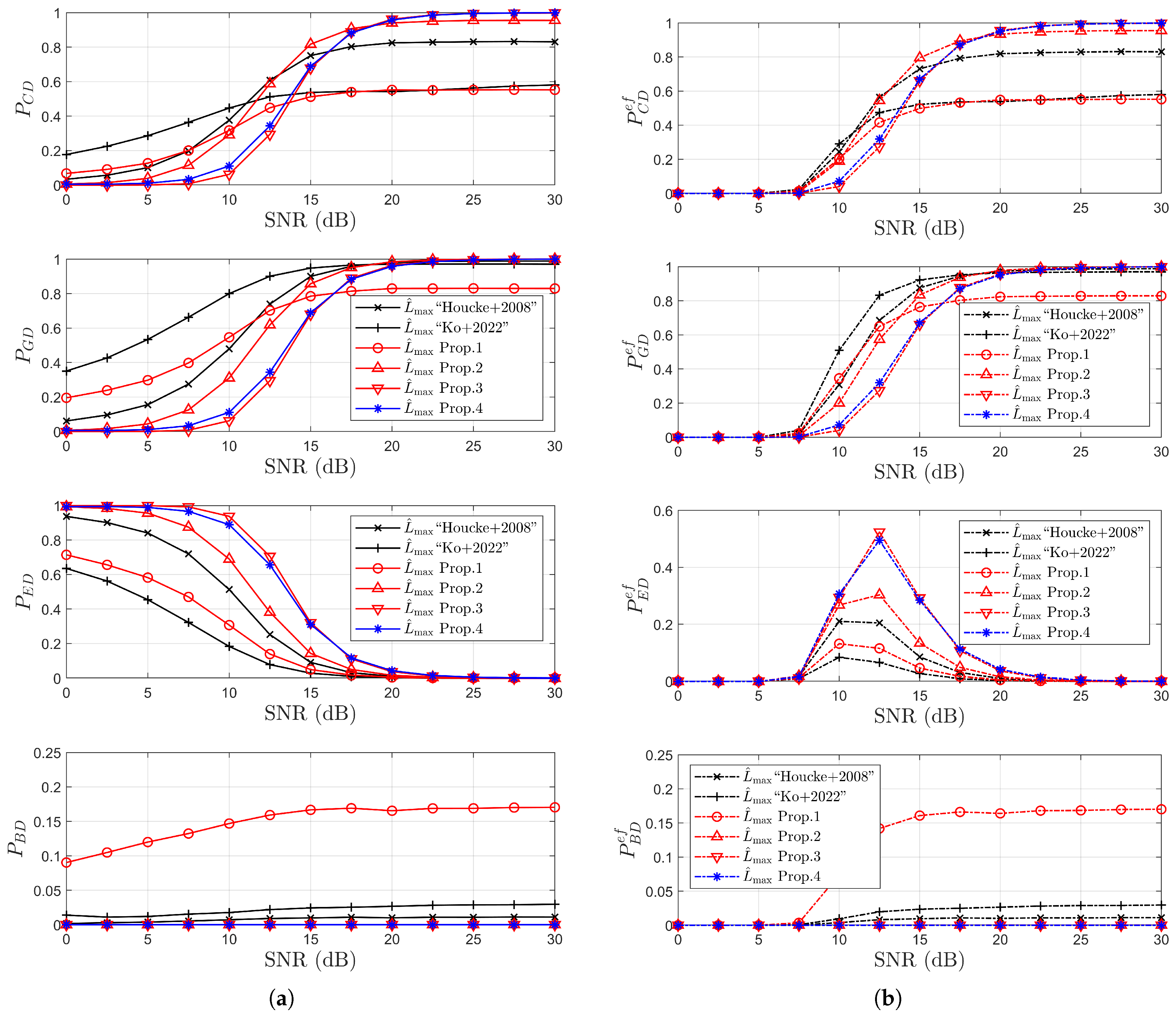
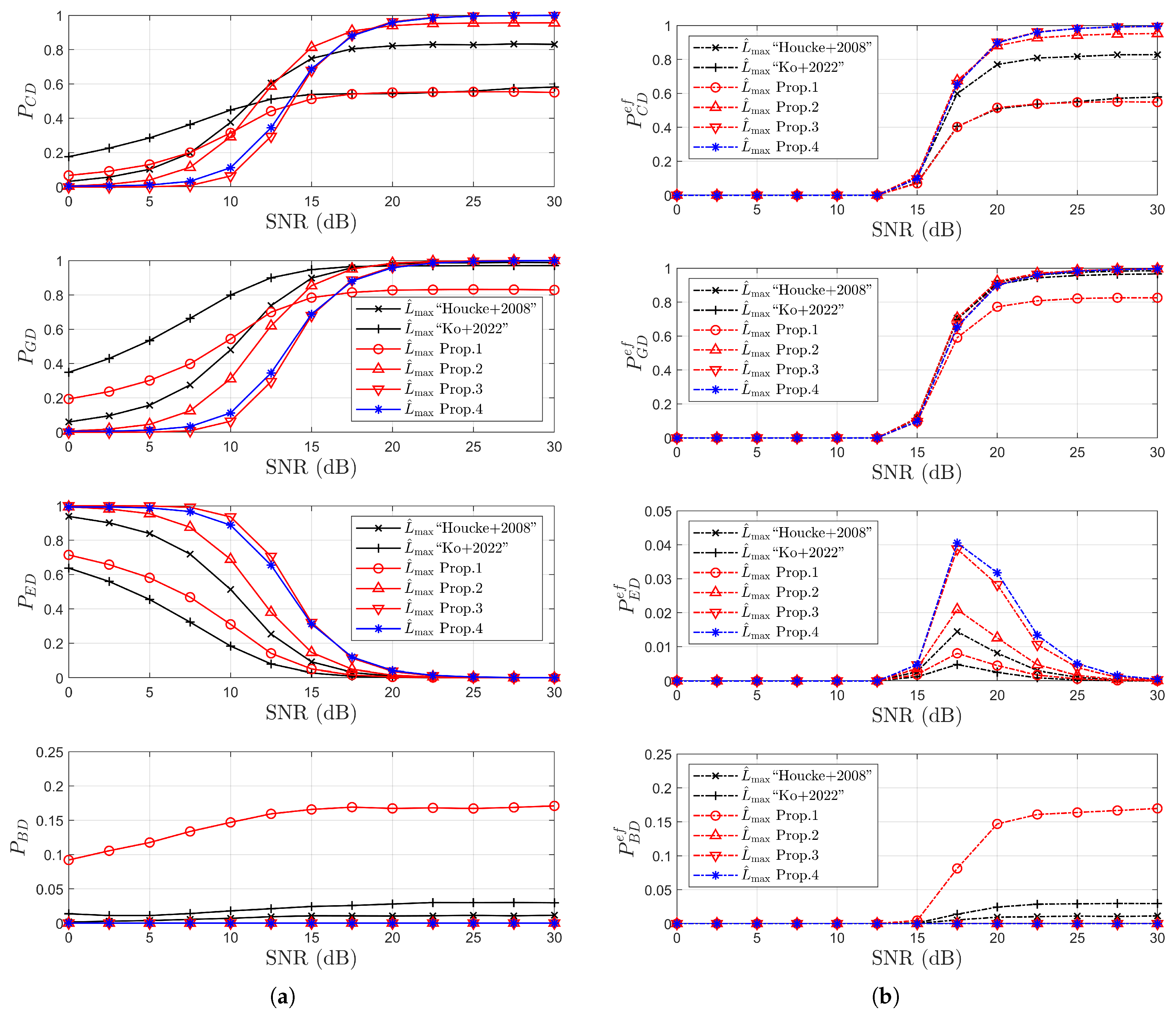
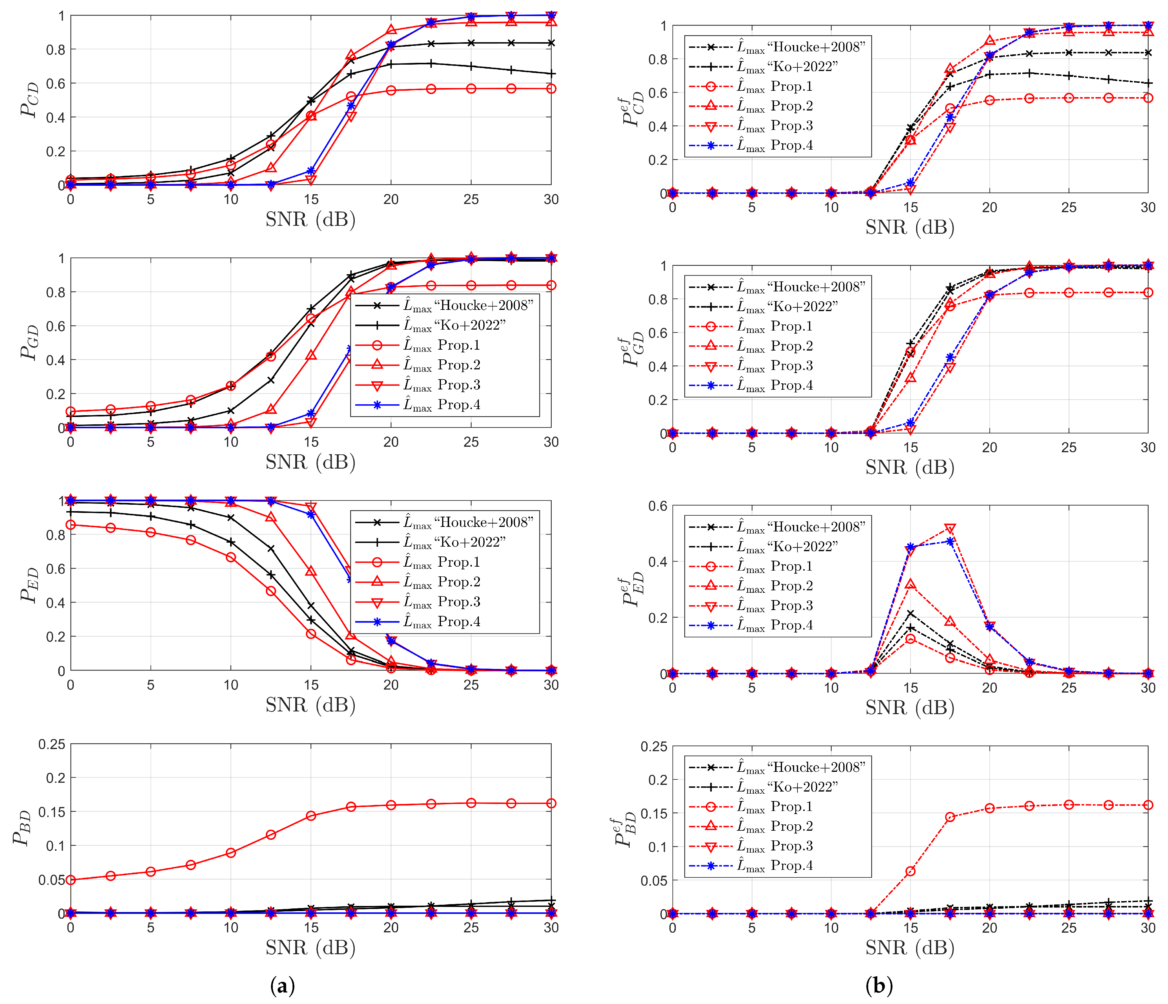
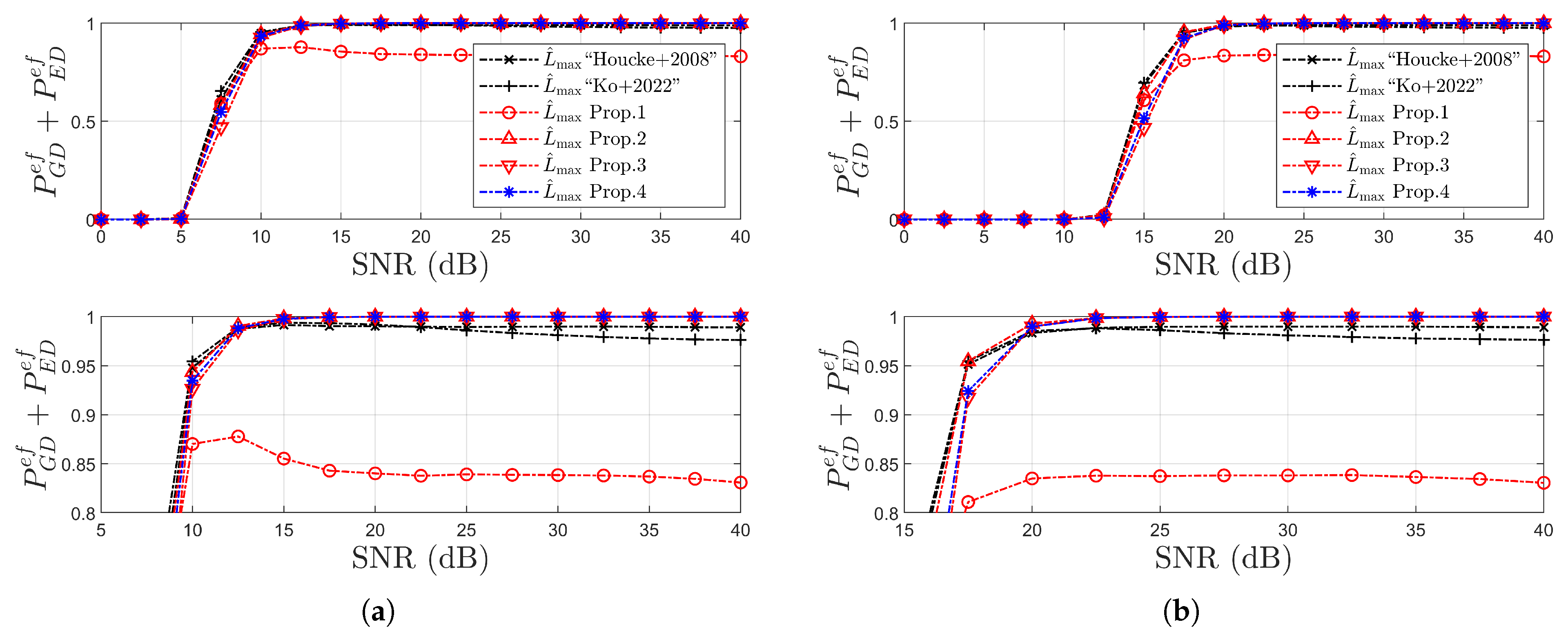
4.1. Simulation Results for Detection Probabilities

From this point, we can define the probabilities of correct detection (CD), good detection (GD), erroneous detection (ED), and bad detection (BD) for ${\widehat{L}}_{max}$, respectively, as follows [7,8]:

$$\begin{array}{cc}\hfill P_{CD}& =\mathrm{Pr}\left\{{\widehat{L}}_{max}=L_{max}\right\}\hfill \\ \hfill P_{GD}& =\mathrm{Pr}\left\{L_{max}\le {\widehat{L}}_{max}<\left(L_{max}+N_g\right)/2\right\}\hfill \\ \hfill P_{ED}& =\mathrm{Pr}\left\{{\widehat{L}}_{max}<L_{max}\right\}\hfill \\ \hfill P_{BD}& =\mathrm{Pr}\left\{\left(L_{max}+N_g\right)/2\le {\widehat{L}}_{max}\right\}\hfill \end{array}$$

(30)

Furthermore, to effectively highlight the advantages of the proposed method, the error-free probability associated with (30) is defined as follows:

$$\begin{array}{cc}\hfill P_{CD}^{ef}& =\mathrm{Pr}\left\{\mathrm{error}-\mathrm{free}\&{\widehat{L}}_{max}=L_{max}\right\}\hfill \\ \hfill P_{GD}^{ef}& =\mathrm{Pr}\left\{\mathrm{error}-\mathrm{free}\&L_{max}\le {\widehat{L}}_{max}<\left(L_{max}+N_g\right)/2\right\}\hfill \\ \hfill P_{ED}^{ef}& =\mathrm{Pr}\left\{\mathrm{error}-\mathrm{free}\&{\widehat{L}}_{max}<L_{max}\right\}\hfill \\ \hfill P_{BD}^{ef}& =\mathrm{Pr}\left\{\mathrm{error}-\mathrm{free}\&\left(L_{max}+N_g\right)/2\le {\widehat{L}}_{max}\right\}\hfill \end{array}$$

(31)

Figure 3, Figure 4 and Figure 5 illustrate the detection probability performance of various CE schemes in the ‘Highway NLOS with 252 km/h’ scenario. Figure 6, Figure 7 and Figure 8 present the detection probability comparison in the ‘Street Crossing NLOS’ scenario at 126 km/h. Figure 9, Figure 10 and Figure 11 show the detection probability results for the ‘Highway LOS’ scenario at 252 km/h. Figure 3a, Figure 6a, and Figure 9a depict the detection probability performance corresponding to (30) for QPSK modulation. Figure 3b, Figure 6b, and Figure 9b show the corresponding error-free detection probability of (31) under the same modulation scheme. Similarly, Figure 4a, Figure 7a, and Figure 10a illustrate the detection probability performance according to (30) for 16QAM modulation. Figure 4b, Figure 7b, and Figure 10b present the error-free detection probability corresponding to (31) for 16QAM. Furthermore, Figure 5a, Figure 8a, and Figure 11a demonstrate the error-free GD+ED probability performance for QPSK modulation. Figure 5b, Figure 8b, and Figure 11b provide a comparative analysis of the error-free GD+ED probability for 16QAM modulation.

In the high-SNR region of the Highway NLOS environment, as shown in Figure 3a and Figure 4a, the proposed methods (from 2 to 4) exhibit higher CD and GD probabilities compared with other methods, while the BD probability remains close to zero. It is noted that a non-zero BD probability can lead to reduced CD and GD probabilities. In the order of ‘${\widehat{L}}_{max}\mathrm{Prop}.1$’, ‘${\widehat{L}}_{max}$ by (27)’, and ‘${\widehat{L}}_{max}\mathrm{Prop}.2$’, the BD probability gradually decreases from a high value and approaches zero. In the low-SNR region of Figure 3a and Figure 4a, the methods in [6,7] appear to exhibit higher CD, GD, and ED performance. It is important to note that the purpose of estimating $L_{max}$ in this paper is to enhance channel estimation performance by enabling interference cancellation based on the estimated value of ${\widehat{L}}_{max}$.

Furthermore, based on the error-free ED probability $P_{ED}^{ef}$ shown in Figure 3b and Figure 4b for the Highway NLOS environment, it can be observed that even when ED events occur in the proposed methods, channel estimation is still performed successfully without error. This situation may occur when the channel power of the last tap in the instantaneous channel is very small, causing $L_{max}$ to be estimated within the ED region. Nevertheless, these cases may still result in error-free symbol detection. Consequently, it is confirmed that the proposed methods utilizing $g\left(l\right)$ in (17) are capable of handling the ED case while minimizing the BD probability to zero as much as possible. A comparison of Figure 3b, Figure 6b, and Figure 9b (as well as Figure 4b, Figure 7b, and Figure 10b) reveals that the error-free ED probability $P_{ED}^{ef}$ increases inversely with the channel power of the last tap, given the specific channel environment.

A similar detection performance trend is observed in both the Street Crossing NLOS (see Figure 6, Figure 7 and Figure 8) and Highway LOS (see Figure 9, Figure 10 and Figure 11) environments. Prop.3 and Prop.4 exhibit nearly identical performance, while Prop.2 outperforms the existing schemes proposed in [6,7]. In contrast, Prop.1 demonstrates inferior detection performance compared with the conventional techniques. In addition, as illustrated in Figure 5, Figure 8, and Figure 11, Prop.1, Prop.2, and Prop.3 demonstrate superior performance compared with the conventional schemes in terms of the error-free GD+ED probability.

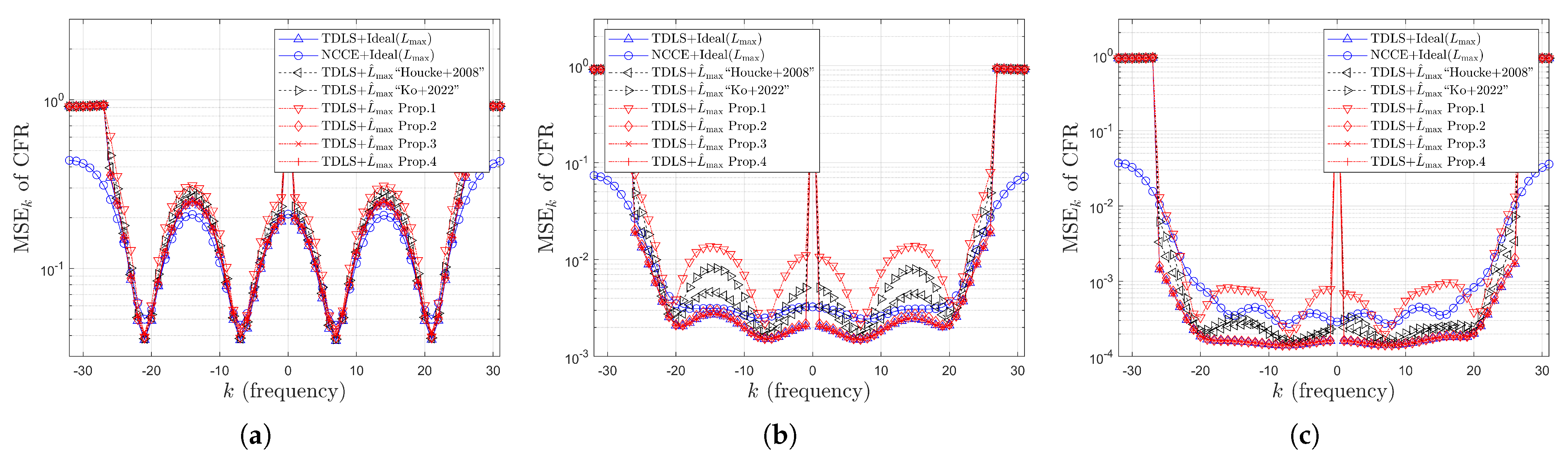
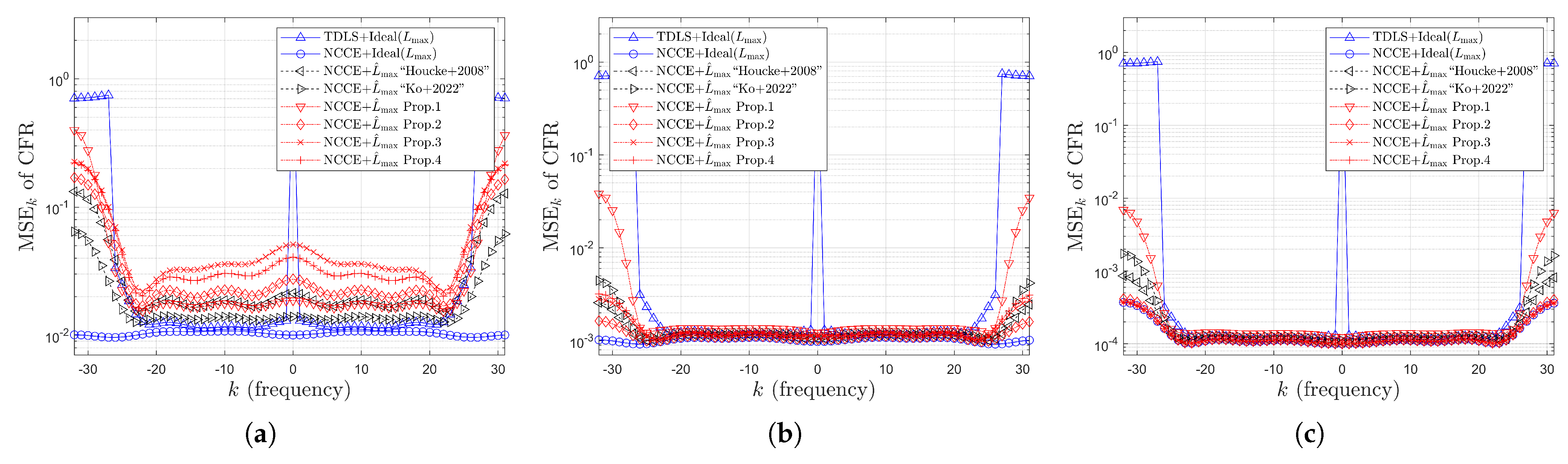
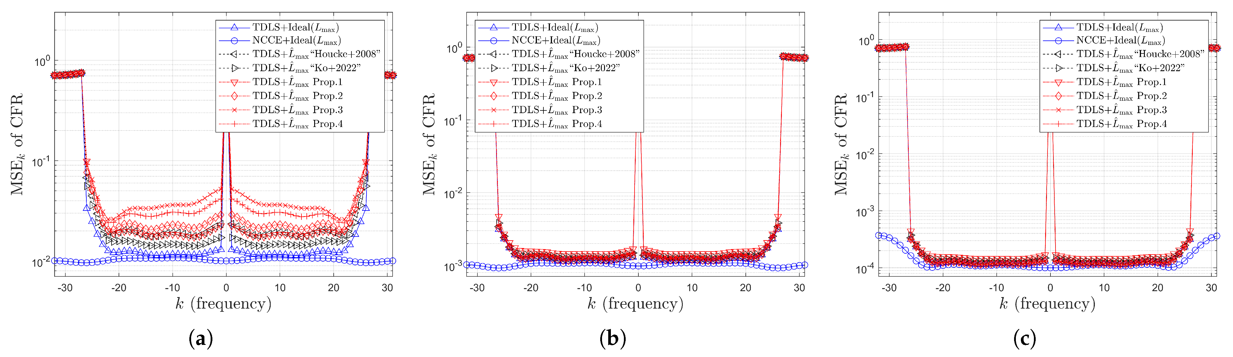
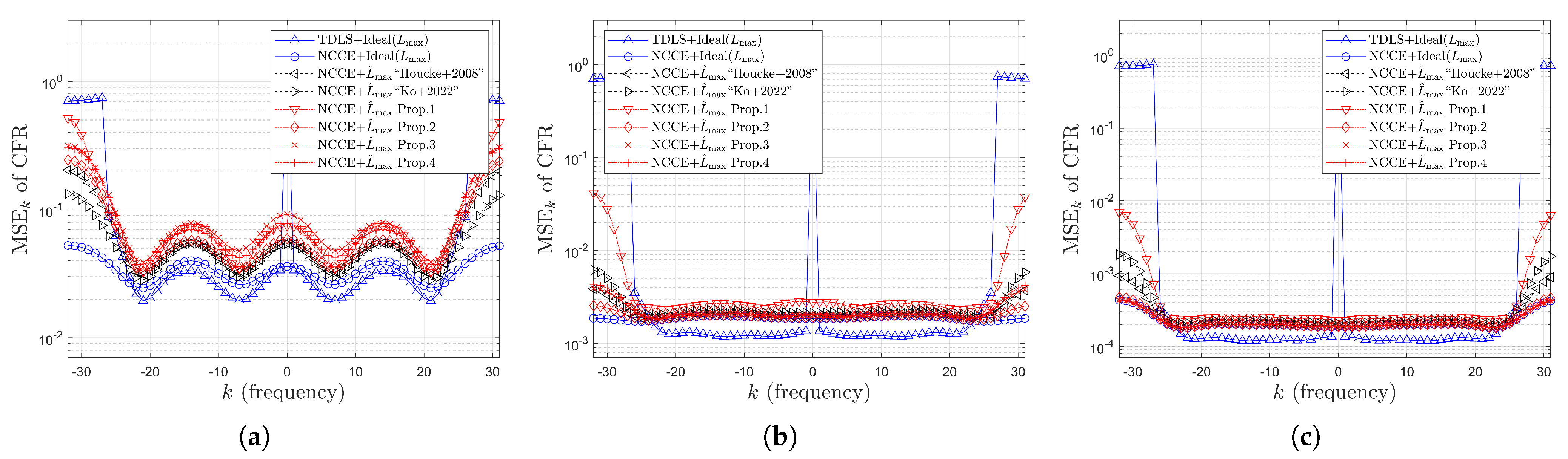
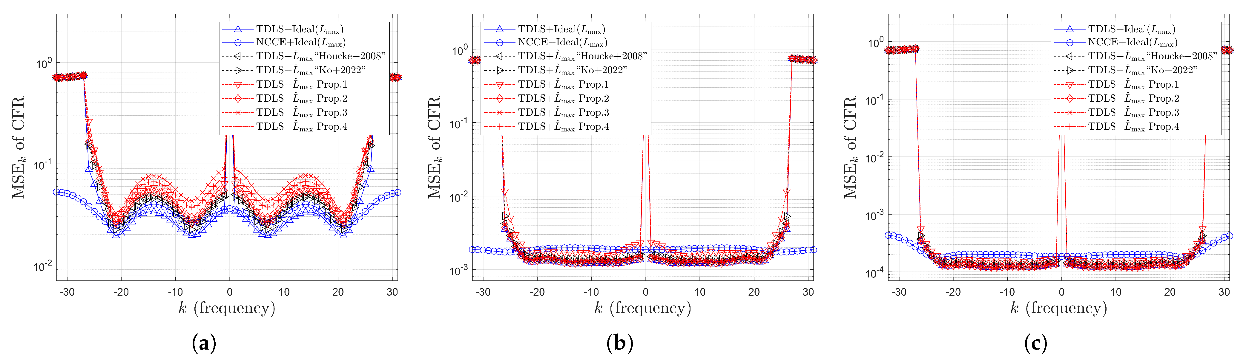
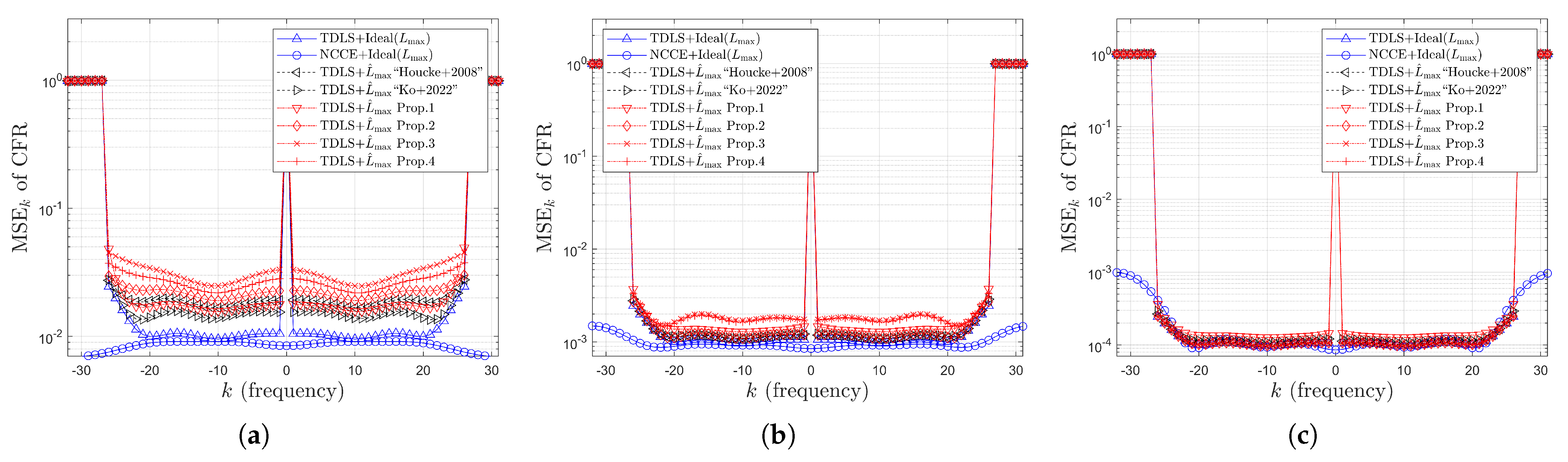
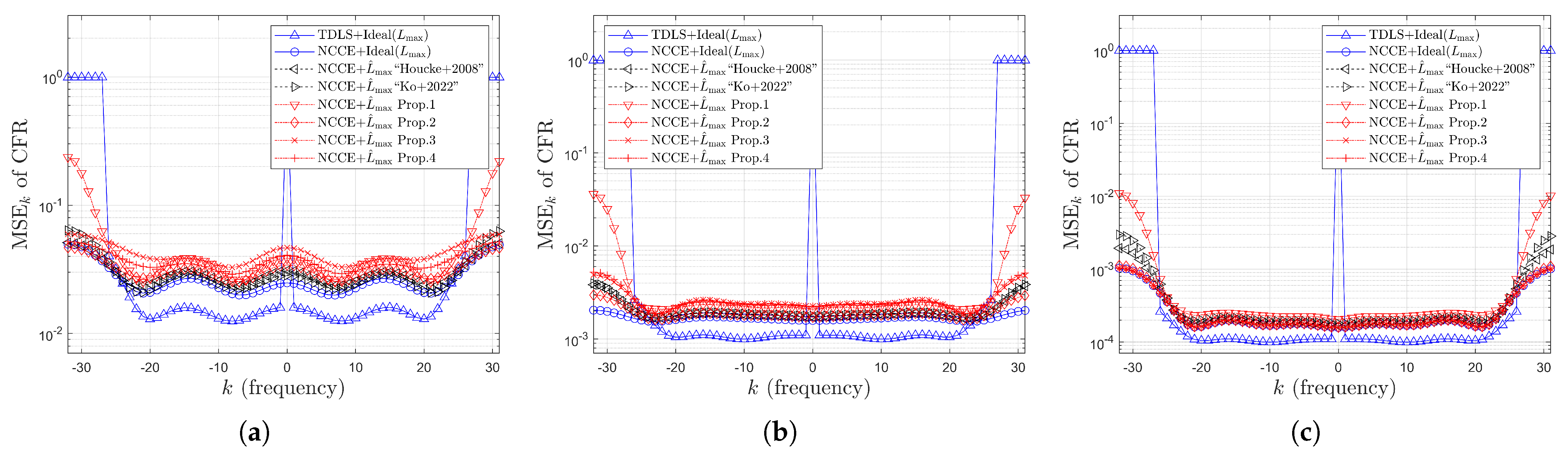
4.2. Simulation Results for MSE

From here, let us define the mean square error (MSE) of the kth CFR and the average MSE (AMSE) of CFRs as

$$\begin{array}{cc}\hfill {\mathrm{MSE}}_k& =E\left[{\left|{\widehat{H}}_i\left(k\right)-H_i\left(k\right)\right|}^2\right]\hfill \\ \hfill \mathrm{AMSE}& ={\displaystyle \frac{1}{N_u}}\sum _{k\in {\mathbb{S}}_u}E\left[{\left|{\widehat{H}}_i\left(k\right)-H_i\left(k\right)\right|}^2\right],\hfill \end{array}$$

where ${\widehat{H}}_i\left(k\right)$ is the estimated kth CFR for the given CE scheme, $H_i\left(k\right)$ is the ideal kth CFR obtained by the FFT on the actual time-varying channel coefficient at the middle position of each OFDM symbol, and ${\mathbb{S}}_u$ is the index set of useful subcarriers for pilot and data subcarriers [13].

Figure 12, Figure 13, Figure 14, Figure 15, Figure 16 and Figure 17 show the AMSE and MSE performance comparison for ‘Highway NLOS with 252 km/h’. Figure 18, Figure 19, Figure 20, Figure 21, Figure 22 and Figure 23 illustrate the AMSE and MSE performance comparison for ‘Street Crossing NLOS with 126 km/h’. Figure 24, Figure 25, Figure 26, Figure 27, Figure 28 and Figure 29 present the AMSE and MSE performance comparison for ‘Highway LOS with 252 km/h’. Figure 12 and Figure 13 compare the AMSE performance of various CE schemes for QPSK and 16QAM for ‘Highway NLOS with 252 km/h’. Figure 18 and Figure 19 show the AMSE comparison for ‘Street Crossing NLOS with 126 km/h’. Figure 24 and Figure 25 illustrate the AMSE comparison for ‘Highway LOS with 252 km/h’. Figure 12a, Figure 13a, Figure 18a, Figure 19a, Figure 24a, and Figure 25a illustrate the AMSE performance of the NCCE schemes. Figure 12b, Figure 13b, Figure 18b, Figure 19b, Figure 24b, and Figure 25b present the AMSE comparison of the TDLS schemes. For ‘Highway NLOS with 252 km/h’, the kth CFR MSE results for QPSK and 16QAM are shown in Figure 14, Figure 15, Figure 16 and Figure 17, where the CE is conducted by using the NCCE and TDLS methods in conjunction with different $L_{max}$ estimators. Figure 20, Figure 21, Figure 22 and Figure 23 display the corresponding kth CFR MSE results for the Street Crossing NLOS environment with a velocity of 126 km/h. Similarly, Figure 26, Figure 27, Figure 28 and Figure 29 illustrate the kth CFR MSE results in the Highway LOS scenario at 252 km/h.

For ‘Highway NLOS with 252 km/h’, from Figure 12, Figure 13, Figure 14, Figure 15, Figure 16 and Figure 17, it can be observed that the three proposed schemes (i.e., red lines corresponding to Prop.2–Prop.4) outperform the two existing schemes (black lines). Furthermore, the proposed schemes (Prop.2–Prop.4) are shown to achieve the MSE bounds (blue lines) of ‘TDLS+Ideal$\left(L_{max}\right)$’ and ‘NCCE+Ideal$\left(L_{max}\right)$’. In Figure 12a and Figure 13a, the NCCE combined with the proposed scheme exhibits saturated AMSE performance. Note that at a low SNR (i.e., SNR = 10 dB), ‘NCCE+Ideal$\left(L_{max}\right)$’ yields a lower MSE than ‘TDLS+Ideal$\left(L_{max}\right)$’ due to the assistance of the estimated CFRs for virtual subcarriers. Conversely, at a high SNR (i.e., SNR = 30 dB), NCCE schemes tend to exhibit saturated MSE performance for virtual subcarriers, allowing TDLS schemes to outperform their NCCE counterparts. As shown in Figure 14c and Figure 15c, the MSE difference between NCCE and TDLS is the most pronounced under these conditions. Moreover, this disparity becomes more significant near the edges of the virtual subcarrier band and in higher-order modulation scenarios such as 16QAM, as observed by comparing Figure 16c and Figure 17c.

The AMSE and the kth MSE performances are generally observed to be similar in both the Street Crossing NLOS (see Figure 18, Figure 19, Figure 20, Figure 21, Figure 22 and Figure 23) and Highway LOS (see Figure 24, Figure 25, Figure 26, Figure 27, Figure 28 and Figure 29) environments. In general, Prop.2 demonstrates performance that is comparable or superior to the two existing schemes across all three channel scenarios. However, Prop.3 and Prop.4 may exhibit inferior AMSE and kth MSE performance when the SNR falls below a certain threshold in both the Street Crossing NLOS and Highway LOS scenarios. Consequently, the robustness of the Prop.2 scheme is evident across various channel conditions.

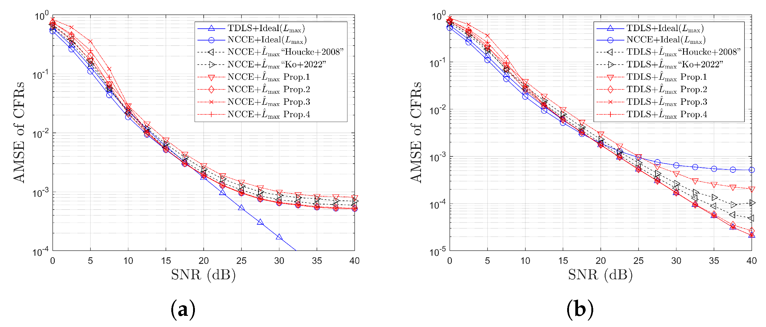
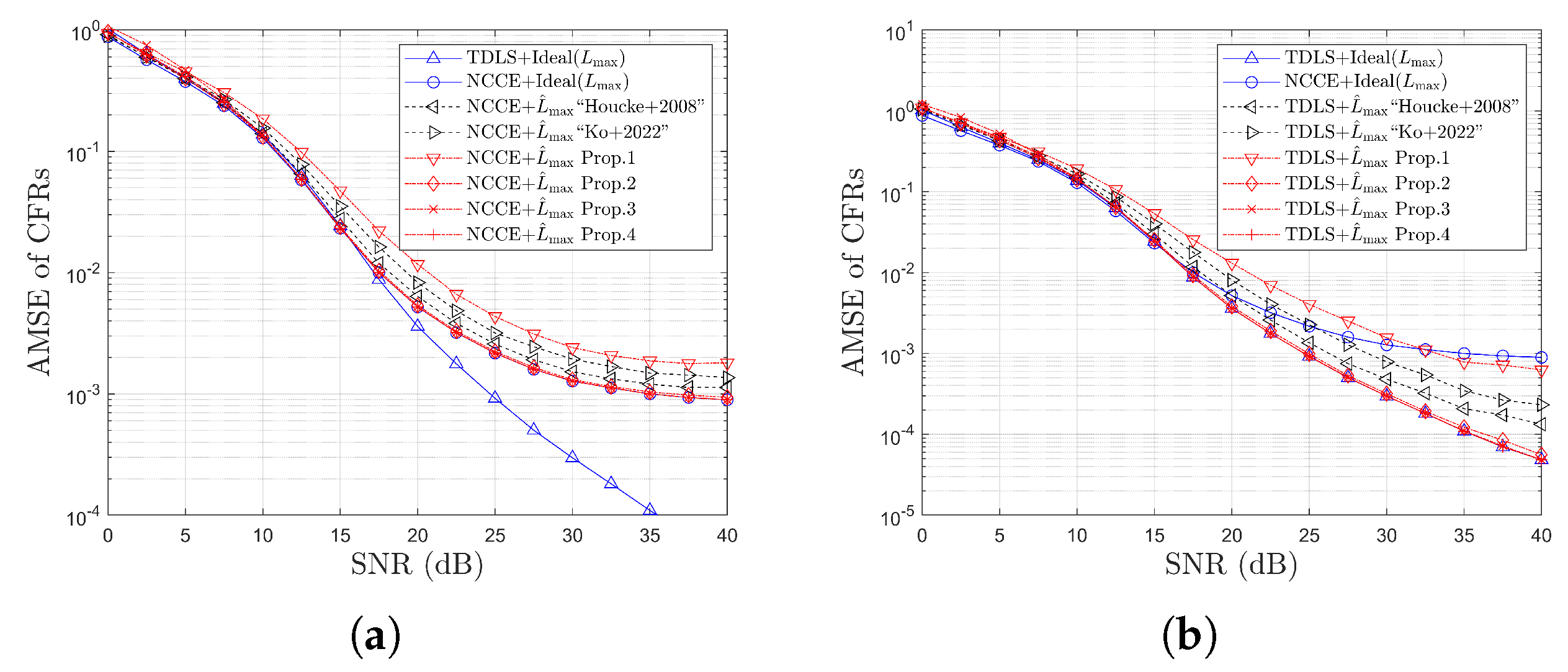
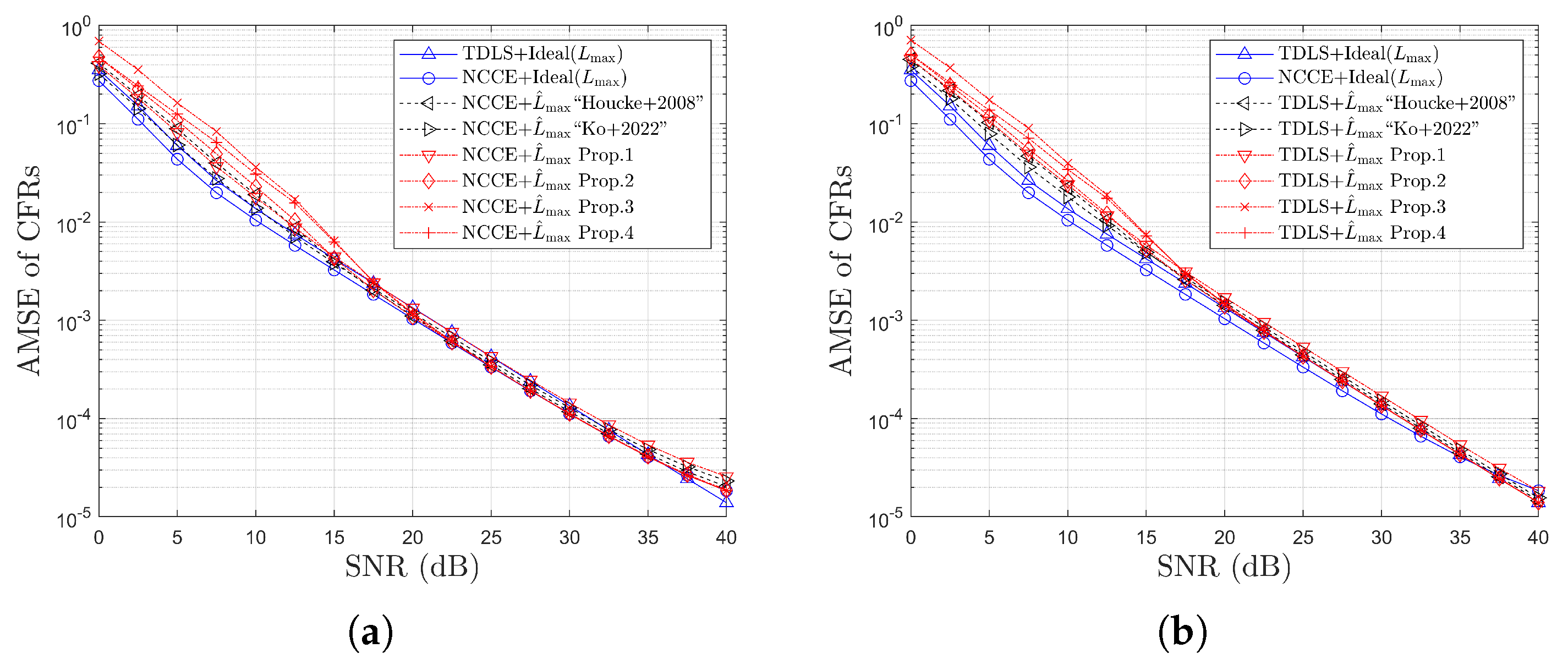
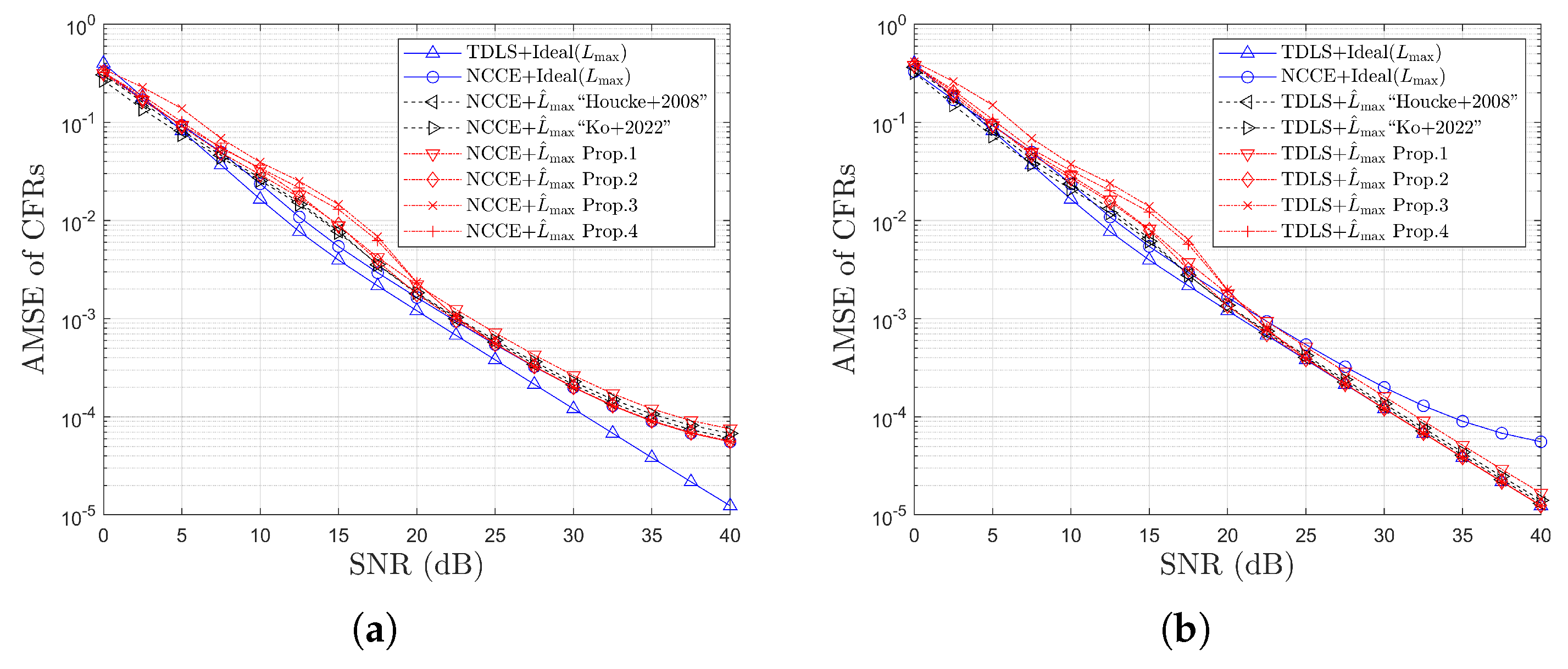
4.3. Simulation Results for Error Rates

Figure 30 and Figure 31 illustrate the PER performance comparison of various CE schemes in the ‘Highway NLOS’ scenario at a velocity of 252 km/h for QPSK and 16QAM, respectively. Figure 32 and Figure 33 present the PER performance comparison in the ‘Street Crossing NLOS’ scenario at 126 km/h for QPSK and 16QAM, respectively. Figure 34 and Figure 35 show the PER performance in the ‘Highway LOS’ scenario at 252 km/h for QPSK and 16QAM, respectively. Figure 30a, Figure 31a, Figure 32a, Figure 33a, Figure 34a, Figure 35a illustrate the error rate performance of the NCCE scheme. Figure 30b, Figure 31b, Figure 32b, Figure 33b, Figure 34b, Figure 35b present the performance of the TDLS scheme. Figure 30c, Figure 31c, Figure 32c, Figure 33c, Figure 34c, Figure 35c provide a comparative analysis of both NCCE and TDLS schemes.

In the ‘Highway NLOS’ scenario, Figure 30 shows the error rate performance comparison for QPSK with respect to $L_{max}$ estimation schemes within both NCCE and TDLS. Figure 31 illustrates the error rate performance comparison for 16QAM with respect to $L_{max}$ estimation schemes under both NCCE and TDLS frameworks. In Figure 30 and Figure 31, it can be observed that the three proposed schemes (i.e., red lines corresponding to Prop.2–Prop.4) outperform the two existing schemes (black lines) and closely approach the error performance bounds (blue lines) of ‘TDLS+Ideal$\left(L_{max}\right)$’ and ‘NCCE+Ideal$\left(L_{max}\right)$’. As mentioned earlier, NCCE results in higher MSE near the virtual subcarriers, as shown in Figure 14c, Figure 15c, Figure 16c, leading to a saturated AMSE of approximately ${10}^{-3}$ in Figure 12a and Figure 13a. Consequently, Figure 30a and Figure 31a reveal a packet error floor in the case of NCCE. At $\mathrm{PER}={10}^{-2}$ for QPSK, it is confirmed that the proposed schemes (Prop.2–Prop. 4) achieve SNR gains of 1.0 dB and 0.5 dB over the scheme in [6] under NCCE and TDLS, respectively. For 16QAM, $\mathrm{PER}={10}^{-2}$ cannot be achieved with NCCE. However, the 0.8 dB SNR gain is observed with TDLS. The SNR gains achieved by Prop.2–Prop.4 over the ${\widehat{L}}_{max}$–based approach in [6] are summarized in

Table 4. SNR gain (dB) of Prop.2–Prop.4 over ${\widehat{L}}_{max}$ in [6].

Environment	CE Scheme	At PER = 10−2	From
Highway NLOS, QPSK	NCCE	1.0 dB	Figure 30c
Highway NLOS, QPSK	TDLS	0.5 dB	Figure 30c
Highway NLOS, 16QAM	TDLS	0.8 dB	Figure 31c

. It is worth noting that the SNR gain can be achieved without additional computational complexity by applying $g\left(l\right)$ in (17). In other words, this gain can be obtained by appropriately adjusting the bias term $B_u$ in (22).

In both the Street Crossing NLOS and Highway LOS scenarios, no packet error floor is observed, even in the case of NCCE (see Figure 32a, Figure 33a, Figure 34a, Figure 35a). It is noteworthy that in the Street Crossing NLOS scenario, both $L_{max}$ and the velocity are lower than those in the Highway NLOS scenario. In this relatively more favorable channel environment, Prop.2–Prop.4 exhibit ER performance comparable to that of the existing methods (see Figure 32c and Figure 33c). On the other hand, the Highway LOS scenario has a smaller $L_{max}$ compared with the Highway NLOS scenario. Figure 34c and Figure 35c illustrate that Prop.2 achieves ER performance similar to that of the existing methods.

By comparing the ER performance across the three channel environments, it can be inferred that the adaptive selection of $g\left(l\right)$ is feasible. Specifically, Prop. 2 to Prop. 4 are more effective in challenging channel conditions where $L_{max}$ is relatively large (i.e., the Highway NLOS scenario), while Prop. 2 alone is sufficient in environments characterized by a shorter $L_{max}$ (i.e., the Street Crossing NLOS and Highway LOS scenarios). Consequently, as discussed in Section 4.2, the robustness of the Prop.2 scheme is evident across various channel conditions.

5. Conclusions

In this paper, an enhanced maximum access delay time estimation method for OFDM systems operating over multipath fading channels has been proposed. By formulating a novel LLR based on the correlation properties introduced by the CP, the proposed scheme effectively approximates the ML estimation of MADT. The generality of the proposed framework has been analytically validated by showing that the existing method represents a special case within it.

Comprehensive simulation results demonstrate that the proposed estimator significantly improves MADT detection performance in terms of correct and good detection probabilities. Furthermore, when applied to the NCCE and TDLS techniques, the proposed MADT estimator enhances overall channel estimation accuracy, approaching the performance of ideal MADT scenarios. These results highlight the practical effectiveness of the proposed approach in realistic vehicular communication environments such as IEEE 802.11p/OFDM systems.

Future research directions include the development of a channel length estimation technique that fully exploits the CP-based correlation properties of the noise estimator, thereby enhancing the robustness of channel parameter estimation. Additionally, as demonstrated in this work, the NCCE technique shows inferior performance compared with TDLS in terms of PER. Therefore, another promising research direction is to design an improved NCCE channel estimation algorithm that can overcome this limitation and further close the performance gap.

As another promising direction for future research, the estimation of the maximum delay spread and the number of channel taps using deep learning approaches, particularly long short-term memory (LSTM) architectures, merits comprehensive investigation. Given the LSTM network’s ability to capture long-range temporal dependencies, it is well-suited for learning channel characteristics from sequential data such as channel state information (CSI) or pilot signal observations. In dynamic V2X communication environments, where the channel properties vary rapidly and non-linearly, LSTM-based models could be trained to estimate either the effective tap count as a regression task or the underlying channel model as a classification task. This unified framework would enable the simultaneous inference of both the tap structure and the channel type, thereby enhancing the adaptability and robustness of wireless communication systems under diverse and time-varying propagation conditions.

References

1. Zhao, Z.; Cheng, X.; Wen, M.; Jiao, B.; Wang, C.X. Channel Estimation Schemes for IEEE 802.11p Standard. IEEE Intell. Transp. Syst. Mag. 2013, 5, 38–49. [Google Scholar] [CrossRef]
2. IEEE Std. 1609.0-2013; IEEE Guide for Wireless Access in Vehicular Environments (WAVE)-Architecture. IEEE: Piscataway, NJ, USA, 2014.
3. Bourdoux, A.; Cappelle, H.; Dejonghe, A. Channel Tracking for Fast Time-Varying Channels in IEEE802.11p Systems. In Proceedings of the 2011 IEEE Global Telecommunications Conference—GLOBECOM 2011, Houston, TX, USA, 5–9 December 2011; pp. 1–6. [Google Scholar]
4. Lim, S. A New Channel Estimation Scheme Using Virtual Subcarriers based on Successive Interpolation in IEEE 802.11p WAVE Systems. In Proceedings of the 2021 International Conference on Convergence Content (ICCC 2021), Jeju, Republic of Korea, 19–20 December 2021; pp. 441–442. [Google Scholar]
5. Han, S.; Park, J.; Song, C. Virtual Subcarrier Aided Channel Estimation Schemes for Tracking Rapid Time Variant Channels in IEEE 802.11p Systems. In Proceedings of the 2020 IEEE 91st Vehicular Technology Conference (VTC2020-Spring), Antwerp, Belgium, 25–28 May 2020; pp. 1–5. [Google Scholar]
6. Socheleau, F.; Aissa-El-Bey, A.; Houcke, S. Non data-aided SNR estimation of OFDM signals. IEEE Commun. Lett. 2008, 12, 813–815. [Google Scholar] [CrossRef]
7. Wang, H.; Lim, S.; Ko, K. Improved Maximum Access Delay Time, Noise Variance, and Power Delay Profile Estimations for OFDM Systems. KSII Trans. Internet Inf. Syst. 2022, 16, 4099–4113. [Google Scholar]
8. Lim, S.; Wang, H.; Ko, K. Power-Delay-Profile-Based MMSE Channel Estimations for OFDM Systems. Electronics 2023, 12, 510. [Google Scholar] [CrossRef]
9. Kim, Y.; Oh, J.; Shin, Y.; Mun, C. Time and frequency domain channel estimation scheme for IEEE 802.11p. In Proceedings of the 17th International IEEE Conference on Intelligent Transportation Systems (ITSC), Qingdao, China, 8–11 October 2014; pp. 1085–1090. [Google Scholar]
10. Kwak, K.; Lee, S.; Kim, J.; Hong, D. A New DFT-Based Channel Estimation Approach for OFDM with Virtual Subcarriers by Leakage Estimation. IEEE Trans. Wirel. Commun. 2008, 7, 2004–2008. [Google Scholar] [CrossRef]
11. Kim, K.; Hwang, H.; Choi, K.; Kim, K. Low-Complexity DFT-Based Channel Estimation with Leakage Nulling for OFDM Systems. IEEE Commun. Lett. 2014, 18, 415–418. [Google Scholar] [CrossRef]
12. Cho, Y.; Son, H. Enhanced DFT-Based Channel Estimator for Leakage Effect Mitigation in OFDM Systems. IEEE Commun. Lett. 2019, 23, 875–879. [Google Scholar] [CrossRef]
13. Ko, K.; Wang, H. Noise-Canceling Channel Estimation Schemes Based on the CIR Length Estimation for IEEE 802.11p/OFDM Systems. Electronics 2024, 13, 1110. [Google Scholar] [CrossRef]
14. Ko, K.; Park, M.; Hong, D. Performance Analysis of Asynchronous MC-CDMA systems with a Guard Period in the form of a Cyclic Prefix. IEEE Trans. Commun. 2006, 2, 216–220. [Google Scholar]
15. Park, M.; Ko, K.; Park, B.; Hong, D. Effects of asynchronous MAI on average SEP performance of OFDMA uplink systems over frequency-selective Rayleigh fading channels. IEEE Trans. Commun. 2010, 2, 586–599. [Google Scholar]
16. Kwak, K.; Lee, S.; Min, H.; Choi, S.; Hong, D. New OFDM Channel Estimation with Dual-ICI Cancellation in Highly Mobile Channel. IEEE Trans. Wirel. Commun. 2010, 10, 3155–3165. [Google Scholar]
17. Cui, T.; Tellambura, C. Power delay profile and noise variance estimation for OFDM. IEEE Commun. Lett. 2006, 1, 25–27. [Google Scholar]
18. van de Beek, J.; Sandell, M.; Borjesson, P. ML estimation of time and frequency offset in OFDM systems. IEEE Trans. Signal Process 1997, 7, 1800–1805. [Google Scholar]
19. Popoulis, A.; Pillai, S. Probability, Random Variables, and Stochastic Processes, 4th ed.; McGraw Hill: Boston, MA, USA, 2002. [Google Scholar]
20. Kahn, M. IEEE 802.11 Regulatory SC DSRC Coexistence Tiger Team V2V Radio Channel Models. Doc.: IEEE 802.11-14, February 2014. Available online: https://mentor.ieee.org/802.11/dcn/14/11-14-0259-00-0reg-v2v-radio-channel-models.ppt (accessed on 22 October 2022).
Figure 1. Example for PDF in (15) and LLR in (16) ( SNR = 10 dB , N g = 16 , L max = 8 , Highway NLOS, 252 km/h, QPSK, CR = 1/2, M = 100 ).
Electronics 14 02404 g001
Figure 2. Example for cost functions ( SNR = 10 dB , Λ u ϵ by g ( l ) = N g l + 1 , N g = 16 , L max = 8 , Highway NLOS, 252 km/h, QPSK, CR = 1/2, M = 100 ).
Electronics 14 02404 g002
Figure 3. Detection probability and error-free detection probability for L max with QPSK for Highway NLOS (252 km/h, L max = 8 , CR = 1/2, M = 100 ): (a) detection probability vs. SNR (dB) and (b) error-free detection probability vs. SNR (dB).
Electronics 14 02404 g003
Figure 4. Detection probability and error-free detection probability for L max with 16QAM for Highway NLOS (252 km/h, L max = 8 , CR = 1/2, M = 100 ): (a) detection probability vs. SNR (dB) and (b) error-free detection probability vs. SNR (dB).
Electronics 14 02404 g004
Figure 5. Error-free GD+ED probability for L max for Highway NLOS (252 km/h, L max = 8 , CR = 1/2, M = 100 ): (a) QPSK and (b) 16QAM.
Electronics 14 02404 g005
Figure 6. Detection probability and error-free detection probability for L max with QPSK for Street Crossing NLOS (126 km/h, L max = 7 , CR = 1/2, M = 100 ): (a) detection probability vs. SNR (dB) and (b) error-free detection probability vs. SNR (dB).
Electronics 14 02404 g006
Figure 7. Detection probability and error-free detection probability for L max with 16QAM for Street Crossing NLOS (126 km/h, L max = 7 , CR = 1/2, M = 100 ): (a) detection probability vs. SNR (dB) and (b) error-free detection probability vs. SNR (dB).
Electronics 14 02404 g007
Figure 8. Error-free GD+ED probability for L max for Street Crossing NLOS (126 km/h, L max = 7 , CR = 1/2, M = 100 ): (a) QPSK and (b) 16QAM.
Electronics 14 02404 g008
Figure 9. Detection probability and error-free detection probability for L max with QPSK for Highway LOS (252 km/h, L max = 6 , CR = 1/2, M = 100 ): (a) detection probability vs. SNR (dB) and (b) error-free detection probability vs. SNR (dB).
Electronics 14 02404 g009
Figure 10. Detection probability and error-free detection probability for L max with 16QAM for Highway LOS (252 km/h, L max = 6 , CR = 1/2, M = 100 ): (a) detection probability vs. SNR (dB) and (b) error-free detection probability vs. SNR (dB).
Electronics 14 02404 g010
Figure 11. Error-free GD+ED probability for L max for Highway LOS (252 km/h, L max = 6 , CR = 1/2, M = 100 ): (a) QPSK and (b) 16QAM.
Electronics 14 02404 g011
Figure 12. CFR AMSE comparison for QPSK for Highway NLOS (252 km/h, L max = 8 , CR = 1/2, M = 100 ): (a) NCCE and (b) TDLS.
Electronics 14 02404 g012
Figure 13. CFR AMSE comparison for 16QAM for Highway NLOS (252 km/h, L max = 8 , CR = 1/2, M = 100 ): (a) NCCE and (b) TDLS.
Electronics 14 02404 g013
Figure 14. CFR MSE comparison for QPSK and NCCE for Highway NLOS (252 km/h, L max = 8 , CR = 1/2, M = 100 ): (a) SNR = 10 dB, (b) SNR = 20 dB, and (c) SNR = 30 dB.
Electronics 14 02404 g014
Figure 15. CFR MSE comparison for QPSK and TDLS for Highway NLOS (252 km/h, L max = 8 , CR = 1/2, M = 100 ): (a) SNR = 10 dB, (b) SNR = 20 dB, and (c) SNR = 30 dB.
Electronics 14 02404 g015
Figure 16. CFR MSE comparison for 16QAM and NCCE for Highway NLOS (252 km/h, L max = 8 , CR = 1/2, M = 100 ): (a) SNR = 10 dB, (b) SNR = 20 dB, and (c) SNR = 30 dB.
Electronics 14 02404 g016
Figure 17. CFR MSE comparison for 16QAM and TDLS for Highway NLOS (252 km/h, L max = 8 , CR = 1/2, M = 100 ): (a) SNR = 10 dB, (b) SNR = 20 dB, and (c) SNR = 30 dB.
Electronics 14 02404 g017
Figure 18. CFR AMSE comparison for QPSK for Street Crossing NLOS (126 km/h, L max = 7 , CR = 1/2, M = 100 ): (a) NCCE and (b) TDLS.
Electronics 14 02404 g018
Figure 19. CFR AMSE comparison for 16QAM for Street Crossing NLOS (126 km/h, L max = 7 , CR = 1/2, M = 100 ): (a) NCCE and (b) TDLS.
Electronics 14 02404 g019
Figure 20. CFR MSE comparison for QPSK and NCCE for Street Crossing NLOS (126 km/h, L max = 7 , CR = 1/2, M = 100 ): (a) SNR = 10 dB, (b) SNR = 20 dB, and (c) SNR = 30 dB.
Electronics 14 02404 g020
Figure 21. CFR MSE comparison for QPSK and TDLS for Street Crossing NLOS (126 km/h, L max = 7 , CR = 1/2, M = 100 ): (a) SNR = 10 dB, (b) SNR = 20 dB, and (c) SNR = 30 dB.
Electronics 14 02404 g021
Figure 22. CFR MSE comparison for 16QAM and NCCE for Street Crossing NLOS (126 km/h, L max = 7 , CR = 1/2, M = 100 ): (a) SNR = 10 dB, (b) SNR = 20 dB, and (c) SNR = 30 dB.
Electronics 14 02404 g022
Figure 23. CFR MSE comparison for 16QAM and TDLS for Street Crossing NLOS (126 km/h, L max = 7 , CR = 1/2, M = 100 ): (a) SNR = 10 dB, (b) SNR = 20 dB, and (c) SNR = 30 dB.
Electronics 14 02404 g023
Figure 24. CFR AMSE comparison for QPSK for Highway LOS (252 km/h, L max = 6 , CR = 1/2, M = 100 ): (a) NCCE and (b) TDLS.
Electronics 14 02404 g024
Figure 25. CFR AMSE comparison for 16QAM for Highway LOS (252 km/h, L max = 6 , CR = 1/2, M = 100 ): (a) NCCE and (b) TDLS.
Electronics 14 02404 g025
Figure 26. CFR MSE comparison for QPSK and NCCE for Highway LOS (252 km/h, L max = 6 , CR = 1/2, M = 100 ): (a) SNR = 10 dB, (b) SNR = 20 dB, and (c) SNR = 30 dB.
Electronics 14 02404 g026
Figure 27. CFR MSE comparison for QPSK and TDLS for Highway LOS (252 km/h, L max = 6 , CR = 1/2, M = 100 ): (a) SNR = 10 dB, (b) SNR = 20 dB, and (c) SNR = 30 dB.
Electronics 14 02404 g027
Figure 28. CFR MSE comparison for 16QAM and NCCE for Highway LOS (252 km/h, L max = 6 , CR = 1/2, M = 100 ): (a) SNR = 10 dB, (b) SNR = 20 dB, and (c) SNR = 30 dB.
Electronics 14 02404 g028
Figure 29. CFR MSE comparison for 16QAM and TDLS for Highway LOS (252 km/h, L max = 6 , CR = 1/2, M = 100 ): (a) SNR = 10 dB, (b) SNR = 20 dB, and (c) SNR = 30 dB.
Electronics 14 02404 g029
Figure 30. Error performance comparison for QPSK for Highway NLOS (252 km/h, L max = 8 , CR = 1/2, M = 100 ): (a) NCCE, (b) TDLS, and (c) NCCE vs. TDLS.
Electronics 14 02404 g030
Figure 31. Error performance comparison for 16QAM for Highway NLOS (252 km/h, L max = 8 , CR = 1/2, M = 100 ): (a) NCCE, (b) TDLS, and (c) NCCE vs. TDLS.
Electronics 14 02404 g031
Figure 32. Error performance comparison for QPSK for Street Crossing NLOS (126 km/h, L max = 7 , CR = 1/2, M = 100 ): (a) NCCE, (b) TDLS, and (c) NCCE vs. TDLS.
Electronics 14 02404 g032
Figure 33. Error performance comparison for 16QAM for Street Crossing NLOS (126 km/h, L max = 7 , CR = 1/2, M = 100 ): (a) NCCE, (b) TDLS, and (c) NCCE vs. TDLS.
Electronics 14 02404 g033
Figure 34. Error performance comparison for QPSK for Highway LOS (252 km/h, L max = 6 , CR = 1/2, M = 100 ): (a) NCCE, (b) TDLS, and (c) NCCE vs. TDLS.
Electronics 14 02404 g034
Figure 35. Error performance comparison for 16QAM for Highway LOS (252 km/h, L max = 6 , CR = 1/2, M = 100 ): (a) NCCE, (b) TDLS, and (c) NCCE vs. TDLS.
Electronics 14 02404 g035