Improved Adaptive Large Neighborhood Search Combined with Simulated Annealing (IALNS-SA) Algorithm for Vehicle Routing Problem with Simultaneous Delivery and Pickup and Time Windows

Abstract

Adaptive Large Neighborhood Search (ALNS) represents a versatile and highly efficient optimization methodology that has demonstrated significant effectiveness in practical applications. This study introduces an enhanced ALNS approach integrated with Simulated Annealing (SA), termed IALNS-SA. The proposed algorithm incorporates supplementary destruction and repair operators within the ALNS framework to augment its robustness and generalization capacity. Additionally, it adopts the SA acceptance criterion to mitigate local optima entrapment. The research investigates the applicability of IALNS-SA to the Vehicle Routing Problem with Simultaneous Delivery and Pickup and Time Windows (VRPSDPTWs), a pivotal challenge in logistics optimization. Through comprehensive evaluation across 56 large-scale benchmark instances, the algorithm’s performance is systematically compared against four established methods: p-SA, DCS, VNS-BSTS, and DGWO. Empirical results indicate that IALNS-SA achieves superior performance relative to DGWO in 69.64% of cases, surpasses VNS-BSTS in 94.64% of instances, and consistently outperforms both p-SA and DCS. The obtained optimal solutions exhibit reduced total vehicle routing distances, thereby substantiating the operational feasibility and algorithmic efficacy of the proposed methodology.

1. Introduction

In recent years, with the deepening of economic globalization, logistics companies have been facing an increasingly competitive environment [1]. To gain a competitive advantage, firms must focus on reducing delivery costs, including fixed vehicle costs, transportation expenses, and other operational overheads [2]. In practical logistics operations, customers typically submit service requests that may involve pickup, delivery, or both simultaneously [3]. Logistics companies group customers based on their geographical locations while also considering constraints such as staff availability and task allocation among customer groups and employees [4]. The ultimate goal is to plan optimal routes for each assigned vehicle, ensuring efficient service from the warehouse to customers and back [5]. Recent advances in metaheuristic algorithms, such as the improved NSGA-II for multi-commodity SDVRP [6], along with emerging research on integrated truck-drone systems [7,8], have demonstrated significant potential for solving such complex routing problems. Genetic algorithm-based approaches, like those proposed by Fazlollahtabar [9] for fuzzy capacitated location-routing problems, show particular promise in addressing these challenges through simultaneous pickup-delivery optimization, while adaptive large neighborhood search methods have shown effectiveness in addressing arc routing challenges in integrated drone-truck systems [10]. Chen et al. (2023) proposed a hybrid optimization framework based on the Pareto front to balance customer satisfaction and vehicle utilization [11]. Sitek et al. (2021) proved through the case of medical material distribution that optimizing VRPSDPTW can reduce the transportation cost by 22% [12]. The cold chain logistics research of Lucq et al. (2023) shows that strict time window control can reduce the spoilage rate of fresh food by 17% [13]. Peng et al. (2024) proposed a dynamic diagnosis method for freight train snaking instability based on trackside multi-sensor fusion and machine learning, and the experimental verification detection accuracy reached 96.7%, which significantly improved the efficiency of railway safety monitoring [14]. Simic et al. (2024) designed a hybrid genetic and Penguin search optimization algorithm (GA-PSEOA), which balanced global exploration and local development through a dynamic adaptive mutation strategy, and shortened the completion time by 12.3% on average and accelerated the convergence by 19% in flow shop scheduling [15]. However, the existing researches still have the following common limitations: (1) Most algorithms rely on fixed operator weights, which are difficult to dynamically adapt to different instance characteristics. (2) Although population algorithms have the advantage of parallel search, they lack efficient local development mechanism, which leads to limited convergence speed [16]. (3) The processing efficiency of large-scale decentralized customer distribution is insufficient, and the utilization rate of vehicle resources is lower than the actual demand [17].

This complex problem is commonly referred to as the Delivery and Pickup Problem (DPP) [18], which has wide-ranging applications in areas such as grocery delivery, parcel distribution, and home healthcare services. When a logistics system must handle both delivery and pickup services simultaneously, the problem is classified as the Vehicle Routing Problem with Simultaneous Delivery and Pickup (VRPSDP) [19,20,21]. Furthermore, if a customer’s pickup and delivery requests must be fulfilled within the same trip, the problem becomes even more intricate [22]. For e-commerce instant delivery, customers are required to complete the pickup and delivery within one hour, and the order distribution is highly dynamic. For medical emergency logistics, it is necessary to complete drug distribution and recycle medical waste within an emergency time window. The case of Sitek et al. (2021) shows that the emergency response time can be reduced by 28% through VRPSDPTW optimization [12]. For cold chain transportation, fresh goods need to be collected and delivered within a strict time window to avoid spoiling, and the route needs to be dynamically adjusted to cope with traffic delays. Lucq et al. (2023) reduced the cost of cargo damage by 12% through the temperate-time window coupling model [13]. For reverse logistics, home appliance recycling needs to coordinate delivery and return pickup in the same path. Reference [16] verifies the contribution of VRPSDPTW to reduce the cost of reverse logistics by 19%. Under specific conditions of VRPSDP, customers may impose service time constraints, such as requiring deliveries or pickups within a designated time window (e.g., between 10:00 AM and 10:30 AM). These constraints introduce an additional layer of complexity, leading to a variant known as the Vehicle Routing Problem with Simultaneous Delivery and Pickup and Time Windows (VRPSDPTWs) [23,24]. Research on this problem is crucial for optimizing logistics distribution efficiency and improving customer satisfaction.

In this context, VRPSDPTW has gained significant attention from both industry practitioners and the academic community. The complexity of this problem arises from the need to optimize not only delivery routes, but also the simultaneous completion of delivery and pickup tasks within specified time windows. Consequently, the study of VRPSDPTW holds substantial theoretical value and practical significance, as it contributes to enhancing the service levels of logistics companies and improving customer satisfaction [25,26]. This research can help enterprises optimize resource allocation, boost operational efficiency, and foster the sustainable development of the logistics industry, thus addressing society’s growing demand for efficient and environmentally friendly logistics services [27,28].

This paper presents an improved Adaptive Large Neighborhood Search algorithm combined with Simulated Annealing (IALNS-SA) to address the Vehicle Routing Problem with Time Windows and Simultaneous Delivery and Pickup (VRPSDPTW). The proposed algorithm operates in three distinct stages: First, it constructs an initial solution using the nearest neighbor heuristic. Second, starting from this initial solution, it generates new local solutions through the Improved Adaptive Large Neighborhood Search (IALNS) algorithm, adaptively adjusting the operation weights based on the quality of the generated solutions. Finally, it applies the Simulated Annealing (SA) acceptance criterion to determine whether to accept the new solutions. By integrating the IALNS algorithm with SA, local search operations are performed on each solution in the solution set, thereby expanding the search space. This approach preserves the perturbation characteristics of IALNS, which help escape local optima, and fully leverages the strengths of the SA algorithm, mitigating the limitations typically associated with the algorithm itself. As a result, it enables an expanded neighborhood search and enhances the quality of the optimal solution. Ultimately, the synergy between these two algorithms improves both the search performance and computational efficiency. The paper concludes with an experimental evaluation using 56 benchmark test instances and compares the results with those of algorithms presented in [29,30,31,32], demonstrating the effectiveness of the proposed approach.

Our research makes the following contributions to the existing Reference: (1) We introduce a novel solution approach, the IALNS-SA algorithm, to address the Vehicle Routing Problem with Time Windows and Simultaneous Delivery and Pickup (VRPSDPTW). (2) We conduct a comprehensive performance ranking of all heuristic methods presented in the Reference and compare their solution quality. (3) We demonstrate that the performance of the IALNS-SA algorithm outperforms the p-SA, DCS, VNS-BSTS, and DGWO algorithms. (4) We provide an in-depth analysis of the components of IALNS-SA, highlighting the importance of each in enhancing the overall solution quality.

The remainder of this paper is organized as follows. Section 2 outlines the problem and establishes the mathematical model. In Section 3, we introduce the IALNS-SA algorithm and describe its components in detail. Section 4 presents the computational experiments, including a comparison of previous methods with IALNS-SA. Finally, Section 5 summarizes our findings and suggests directions for future research.

2. Related Work

2.1. Review of the Vehicle Routing Problem with Simultaneous Delivery and Pickup and Time Windows (VRPSDPTWs)

The Vehicle Routing Problem with Simultaneous Delivery and Pickup and Time Windows (VRPSDPTWs) is an extension of the classic Vehicle Routing Problem (VRP) and is known to be NP-hard [33]. The algorithms designed to solve VRPSDPTW can be broadly categorized into two groups. The first group includes the operation’s research-based methods, such as dynamic programming and branch-and-price techniques [34]. These methods are capable of finding optimal solutions for small-scale problems; however, as the problem size increases, the computational complexity escalates, and these approaches may require several days to obtain a satisfactory solution. The second group consists of intelligent algorithms [11,35,36], including genetic algorithms, ant colony optimization, particle swarm optimization, and others. These algorithms are generally independent of problem size and can often provide satisfactory solutions within a relatively short time frame. Consequently, research on VRPSDPTW, both domestically and internationally, has largely focused on various intelligent algorithms. For example, Sitek et al. [12] proposed an improved hybrid method for solving VRPSDPTW; Kurniawati et al. [13] introduced the ALNS-TS algorithm to address VRPSDPTW; Wang et al. [16] incorporated the condition of multiple distribution centers into VRPSDPTW and employed clustering algorithms to obtain optimal solutions; Wang Chao et al. [29] developed a discretized cuckoo search algorithm to solve VRPSDPTW; Lagos et al. [17] applied an enhanced particle swarm optimization algorithm to optimize VRPSDPTW; and Chen Kai et al. [30] proposed a discrete gray wolf optimization algorithm to effectively tackle VRPSDPTW. These studies suggest that metaheuristic algorithms can provide more effective solutions to VRP. However, in the search process, most of these algorithms rely on fixed local search operations, such as deletion and insertion, which can constrain the search space and often lead to local optima. Therefore, selecting an appropriate algorithm and designing strategies to avoid local optima are critical to improving the performance of these algorithms.

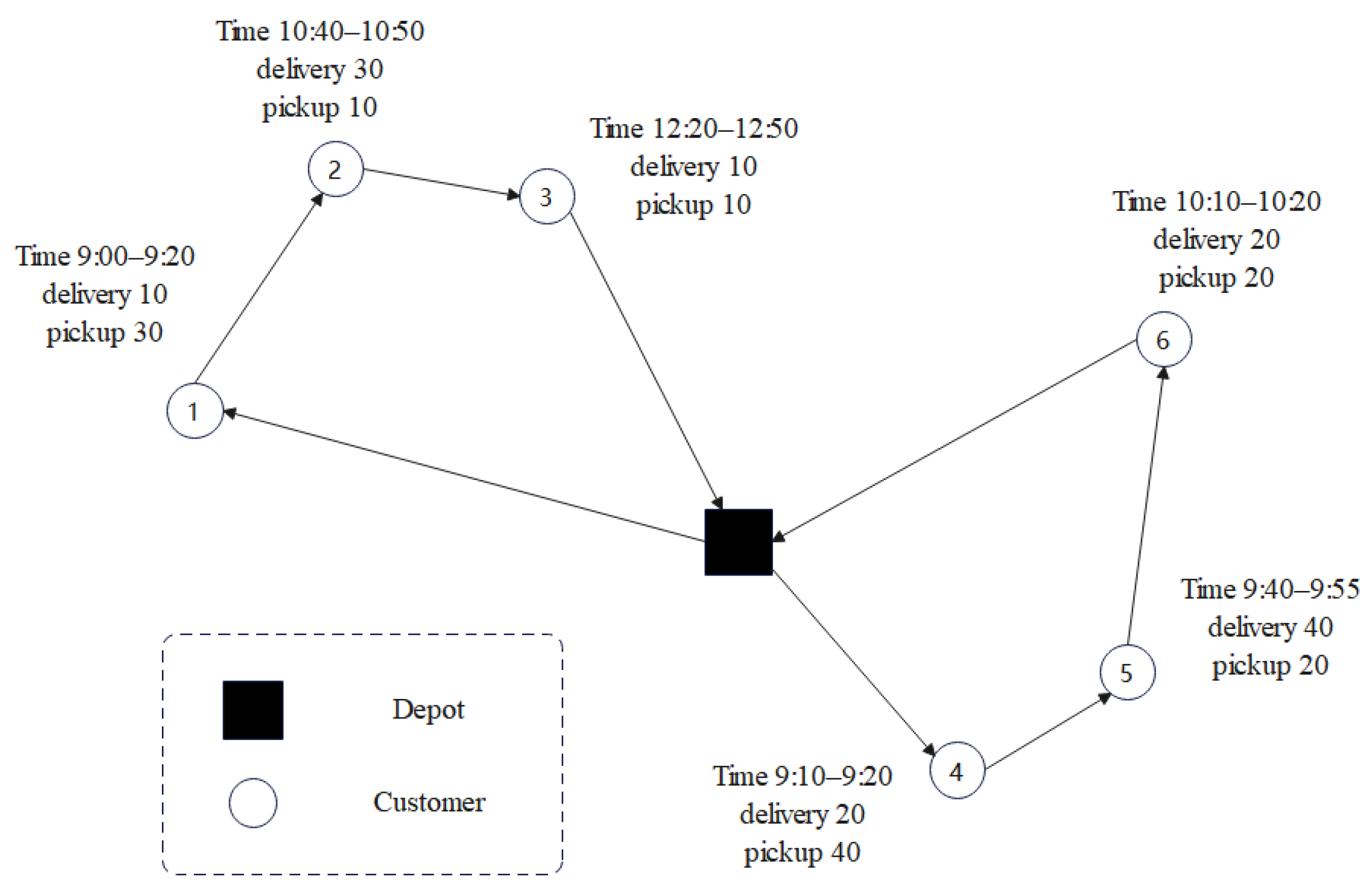
2.2. The Vehicle Routing Problem with Simultaneous Delivery and Pickup and Time Windows (VRPSDPTWs)

VRPSDPTW is illustrated in Figure 1, where the square represents the distribution center, the numbered circles represent the customers, each customer has a specified service time and delivery/pickup quantities, and the arrows indicate the vehicle delivery routes. VRPSDPTW can be defined as follows: Given a directed graph with weights $\mathrm{G}=\left(\mathrm{V},\mathrm{A},\mathrm{C}\right)$, where $\mathrm{V}=\left\{i|i=\mathrm{0,1},\dots ,n,n+1\right\}$ is the set of nodes, with node $0$ and node $n+1$ being the depot node and nodes $\left(1~n\right)$ being customer nodes; $\mathrm{A}=\left\{i,j|i,j\in V\right\}$ denotes the set of arcs, and $\mathrm{C}=\left\{c_{ij}|\left(i, j\right)\in A\right\}$ is the weight matrix, with $c_{ij}$ representing the distance from node $i$ to node $j$. Let there be a delivery demand $p_i$, a pickup demand $d_i$, a left time window ${\mathrm{a}}_i$, a right time window ${\mathrm{b}}_i$, a service time ${\mathrm{s}}_i$ for each customer node $i$, let the maximum cargo capacity of the transport vehicle be $Q$, travel time ${\mathrm{t}}_{ij}$ represents from node $i$ to node $j$, and the left time window $E$ and the right time window $L$ of the distribution center, then we obtain sufficiently large positive numbers $M$. The decision variables include the start service time ${\mathrm{w}}_{ik}$ of the vehicle $k$ at the node $i$, the loading capacity $L_{0k}$ of the vehicle when it leaves the distribution center, the loading capacity $L_i$ of the vehicle after serving customer $i$, and $x_{ijk}$ represents whether the vehicle departs from the node $i$ to another node $j$. In addition, ${∆}^{+}\left(i\right)$ represents the set of arcs departing from the node $j$, ${∆}_{-}\left(i\right)$ represents the set of arcs returning to the node $j$, N = V\{0, n + 1} represents the set of customers, and $K$ represents the set of distribution vehicles. VRPSDPTW can be described as follows: (1) Each vehicle starts from node 0, services several customers, and returns to node 0, forming a solution $S$; (2) Each customer is served exactly once and only by one vehicle; (3) The load of each vehicle does not exceed $Q$; (4) The pickup and delivery demands of each customer do not exceed $Q$; (5) The vehicle must provide service after the left time window; (6) Vehicles are not allowed to arrive after the right time window; (7) The total transportation distance $f\left(S\right)$ is minimized.

2.3. The Vehicle Routing Problem with Simultaneous Delivery and Pickup and Time Windows (VRPSDPDTWs) Mathematical Model

The mathematical model of VRPSDPTW can be described as follows:

$$min{\sum }_{k\in K}{\sum }_{\left(i,j\right)\in A}{c}_{ij}{x}_{ijk}$$

(1)

Constraints:

$${\sum }_{k\in K}{\sum }_{j\in {∆}^{+}\left(i\right)}{x}_{ijk}=1\forall i\in N$$

(2)

$${\sum }_{j\in {∆}^{+}\left(0\right)}{x}_{0jk}=1\forall k\in K$$

(3)

$${\sum }_{i\in {∆}_{-}\left(j\right)}{x}_{ijk}-{\sum }_{i\in {∆}^{+}\left(j\right)}{x}_{jik}=0\forall j\in N,\forall k\in K$$

(4)

$${\sum }_{i\in {∆}_{-}(n+1)}{x}_{i,n+1,k}=1\forall k\in K$$

(5)

$$t_{ij}={\displaystyle \frac{c_{ij}}{v}}$$

(6)

$$w_{ik}+s_i+t_{ij}-w_{jk}\le \left(1-x_{ijk}\right)M\forall \left(i,j\right)\in A,\forall k\in K$$

(7)

$$a_i\left({\sum }_{j\in {∆}^{+}\left(i\right)}{x}_{ijk}\right)\le w_{ik}\le b_i\left({\sum }_{j\in {∆}^{+}\left(i\right)}{x}_{ijk}\right)\forall i\in N,\forall k\in K$$

(8)

$$E\le w_{ik}\le L\forall i\in \left\{0,n+1\right\}\forall k\in K$$

(9)

$$L_{0k}={\sum }_{i\in N}{d}_i{\sum }_{j\in {∆}^{+}\left(i\right)}{x}_{ijk}\forall k\in K$$

(10)

$$L_j\ge L_{0k}-d_j+p_j-M\left(1-x_{0jk}\right)\forall j\in N,\forall k\in K$$

(11)

$$L_j\ge L_i-d_j+p_j-M\left(1-{\sum }_{k\in K}{x}_{ijk}\right)\forall i\in N,\forall j\in N$$

(12)

$$L_{0k}\le C\forall k\in K$$

(13)

$$L_{0k}\le C+M\left(1-{\sum }_{i\in V\left\{0\right\}}{x}_{ijk}\right)\forall j\in N,\forall k\in K$$

(14)

$$x_{ijk}\in \left\{\mathrm{0,1}\right\}\forall \left(i,j\right)\in A,\forall k\in K$$

(15)

2.4. Adaptive Large Neighborhood Search (ALNS)

Ropke and Pisinger [37] introduced the Adaptive Large Neighborhood Search (ALNS) algorithm, which utilizes a diverse set of destruction and repair operators throughout the search process, with one operator being selected per iteration. The selection probability of each operator is based on its historical performance and is updated progressively over iterations. This approach allows ALNS to effectively avoid being trapped in local optima during the optimization process. Additionally, by incorporating heuristic information during the neighborhood search, ALNS is capable of obtaining high-quality solutions with a certain probability.

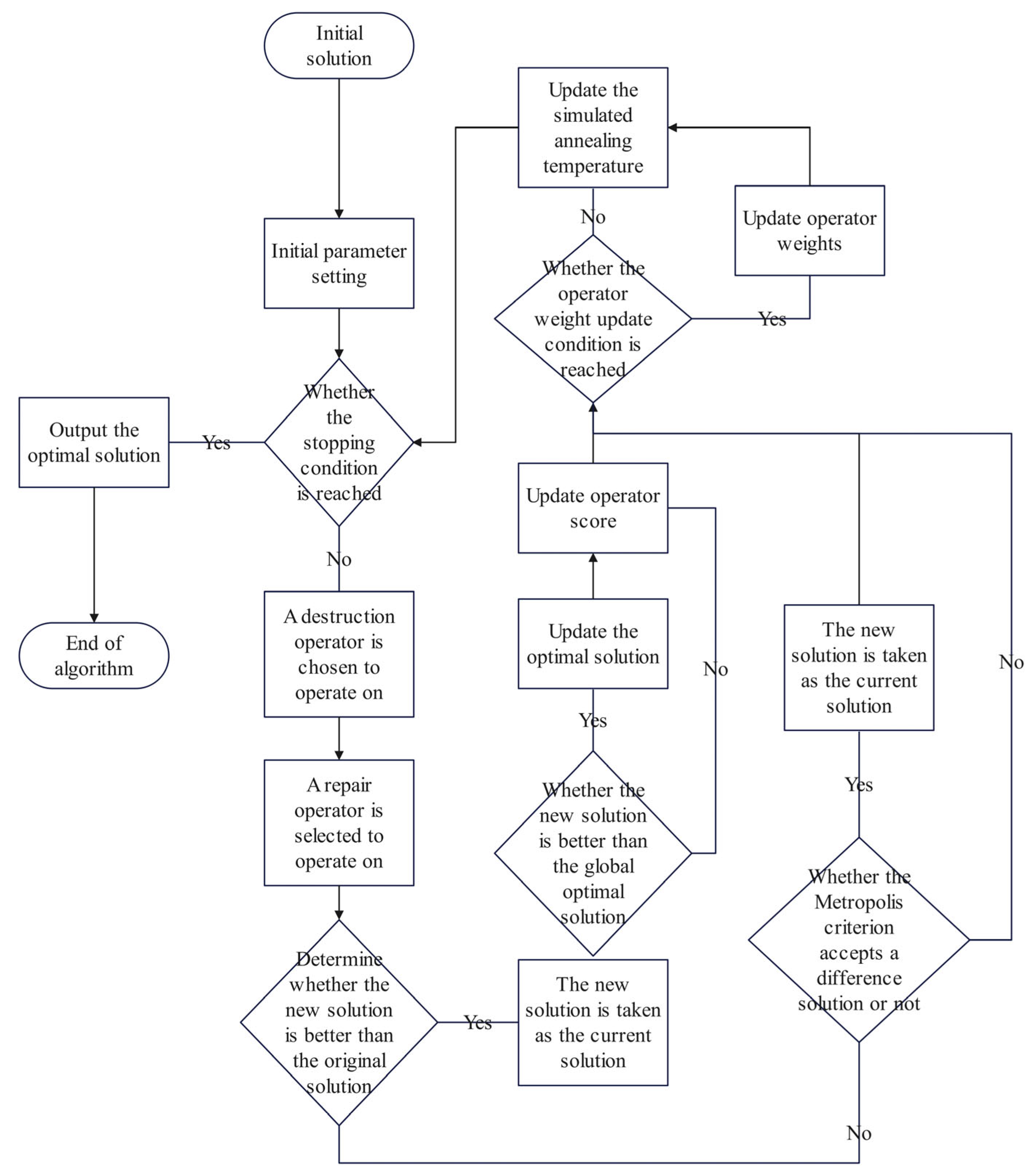
3. Adaptive Large Neighborhood Search Integrated with Simulated Annealing (IALNS-SA) Algorithm

This paper introduces the IALNS-SA algorithm, whose flowchart is depicted in Figure 2. The algorithm integrates Simulated Annealing concepts with Iterated Adaptive Large Neighborhood Search for optimization. Within the IALNS framework, additional destruction and repair operators are incorporated to enhance the algorithm’s flexibility. Specifically, IALNS-SA includes five destruction operators and five repair operators, each of which is assigned a score and a weight. During the neighborhood search process, operators are dynamically selected based on their respective scores and weights. The five destruction operators target specific scenarios such as customer distribution, time window conflicts, and vehicle utilization, ensuring the solution space is fully explored. For instance, the Similarity Destroy Operator optimizes routes for densely clustered customers, while the Random Destroy Operator enhances perturbation capability for dispersed distributions. The repair operators complement these strategies through greedy, global-optimal, and randomized perturbation approaches. For example, the Minimum Insertion Cost Repair Operator rapidly generates feasible solutions, while the Regret Criterion Repair Operator mitigates the risk of local optima. Their combination balances efficiency and solution quality. The Maximum Waiting Time Destroy Operator and Minimum Waiting Time Repair Operator collaboratively address time window conflicts to ensure route feasibility. Similarly, the Destroying Vehicle Operator and Global Optimal Repair Operator synergize to optimize vehicle resource allocation.

The steps of the algorithm are as follows. First, an initial solution is generated using the nearest neighbor heuristic. This initial solution serves as the starting point for the IALNS. Five destruction operators are applied to remove a subset of customer nodes, and subsequently, five repair operators are used to reinsert these customers into the routes, resulting in a new solution. The weights are dynamically adjusted based on the comparison between the new and old solutions. Finally, using the SA acceptance criterion, the algorithm determines whether to accept the new solution. Worse solutions may be accepted with a certain probability, helping to prevent the algorithm from getting trapped in local optima.

3.1. Initialization Solution

In this paper, the initial solution set is constructed using the nearest neighbor heuristic, which is implemented in three steps:

Step 1: Select the customer node closest to the departure node from the set of unvisited customer nodes to initiate a new route.

Step 2: Choose the most appropriate next customer node from the remaining unvisited nodes to extend the current route.

Step 3: Continuously select the customer node closest to the last visited node in the current route until all customers have been assigned to a route.

3.2. Solution Optimization

This paper utilizes the IALNS-SA algorithm for route optimization, which proceeds through the following steps:

Step 1: Select a destruction operator based on the assigned weights to destroy the current solution, resulting in a destroyed solution.

Step 2: Choose a repair operator, also based on its weight, to repair the destroyed solution, generating a new solution.

Step 3: Adjust the weights of the destruction and repair operators based on the quality of the new solution and the solutions stored in memory.

3.2.1. Destroy Operator

Traditional ALNS employs relatively fixed destroy operators, such as Random Destroy Operator and Maximum Saving Cost Destroy Operator, whose strategies typically rely on simple heuristic rules, making them ineffective for handling complex spatio-temporal constraints. In contrast, IALNS-SA introduces novel operators such as Similarity Destroy Operator, Destroying Vehicle Destroy Operator, and Maximum Waiting Time Destroy Operator. These operators deeply integrate the spatio-temporal correlation features of VRPSDPTW. By dynamically adjusting destruction intensity and scope, they precisely identify and relax critical constraints, thereby significantly enhancing efficiency in solving spatio-temporal coupling problems. This paper designs five destruction operators, each employing a distinct destruction method to expand the algorithm’s search space, thereby facilitating the attainment of an optimal solution.

• Random Destroy Operator

By randomly removing customers and forcing path reconstruction, the random destroy operator can cope with the diversity requirements of scattered distributed instances. Reference [11] shows that random perturbation can avoid the premature problem of population algorithm. This operator randomly selects q customers from the path and then removes q customers from the corresponding path positions, aiming to increase the diversity of solutions. In the random destruction operator, the number q of customers removed was dynamically adjusted: the initial reference value was set to q = 0.1 n, and an adaptive mechanism was introduced. If the solution was not improved for 10 consecutive iterations, q was increased to 0.15 n to enhance the disturbance of the algorithm. On the contrary, if a better solution is found five times in a row, q is reduced to 0.05 n to promote the local refined search. In addition, the parameter range was dynamically adapted for different instance types: the upper limit of q was extended to 0.2 n in the dispersed distribution instances to enhance diversity, and the lower limit of q was shrunk to 0.05 n in the concentrated distribution instances to balance the search intensity. For example, by randomly removing customer nodes, the local structure of the current solution is broken, the diversity of the solution is increased, and the algorithm avoids premature focus on a single region, which is suitable for handling the path reconstruction requirements when customers are scattered.

2.

Similarity Destroy Operator

According to the characteristics of dense customer groups, customers with high spatio-temporal correlation are removed, and compact paths are forced to be reorganized to reduce redundant driving. This strategy makes up for the deficiency of single repair strategy of DCS algorithm in reference [24]. The purpose of this operator is to remove a set of points that are similar to some randomly selected point from the current solution. The calculation of similarity takes into account several factors. The random element D in similarity destruction is generated by the following rules: Initially, three customers were randomly selected from the current solution as candidate seeds. If a better solution was generated after removing D associated customers, D was retained to the next iteration, otherwise it was reset to a random new seed. For the time window strict instance, the spatio-temporal weight of Equation (16) is dynamically adjusted (distance weight is reduced to 0.3, time overlap weight is increased to 0.7) to strengthen the priority of time relevance. For example, based on calculating the spatio-temporal correlation between customers (such as distance and service time overlap), it preferentially removes customers with strong correlation, and forces the reorganization of tightly coupled paths, so as to optimize the path compactness of centralized distribution. A number of relevant customers are removed using the following formula:

$$R\left(i,j\right)=1/(c_{ij}^{\mathrm{’}}+V_{ij})$$

(16)

where $c_{ij}^{\mathrm{’}}$ is the normalized value of $c_{ij}$, ranging from [0,1]; $c_{ij}$ is the Euclidean distance between points $i$ and $j$; $V_{ij}$ is a binary indicator of whether i and j are on the same route. It is 0 if $i$ and $j$ are on the same route, otherwise it is 1.

It can be seen from the above formula that the larger $R(i,j)$, the greater the correlation between customer $i$ and customer $j$. Based on the above correlation calculation formula, assuming the number of customers is $N$, the number of customers to be removed is $q$, and the random element is $D$; the pseudocode for the destruction operator is shown as Algorithm 1.

Algorithm 1 Similarity Destroy Operator

Input: Current solution $S$, number of customers to remove $q$, random element $D$ Output: Destroyed solution $S_d$, set of removed customers $I$ Randomly select a customer $i_{seed}$ from the solution $S$, and add $i_{seed}$ to the set $I$ while $\left| I \right|<q$ do Randomly select a customer $i_{curr}$ from the set $I$ Sort the customers that are in the current solution $S$ but not in the set $I$ as follows: $i < j\Rightarrow R(i_{curr}, L[i\left]\right) < R(i_{curr}, L[j\left]\right)$, then store the sorting result in the sequence $L$ Calculate the index of randomly selected customers $k\leftarrow ⌈{rand}^D\left|L\right|⌉$ $I\leftarrow I\cup \left\{L_k\right\}$ end while Remove the customers in the set $I$ from the solution $S$ to obtain the destroyed solution $S_d$ return $S_d$ and $I$

3.

Maximum Saving Cost Destroy Operator

High-cost customers are preferentially removed to alleviate the vehicle capacity shortage scenario, and the efficiency bottleneck of DGWO fixed neighborhood operation in [30] is solved. This operator calculates the distance saved by each customer on the removal path, and selects the point with the largest cost saving to remove until the number q of customers to be removed is reached. The implementation steps of the strategy included the following. First, all customers in the path were searched and their ${∆C}_i$ values were calculated, and then the top q customers were removed by sorting them in descending order of ${∆C}_i$. For the C2 class instances where the vehicle capacity is exceeded, the system will preferentially remove the customers with higher ${∆C}_i$ values that cause the load overrun. The experimental results show that the dynamic removal strategy achieves 12% cost savings on the Cdp107 test instances, which is significantly better than the static removal method proposed in reference [29]. For example, Equation (17) is used to calculate the path distance reduction after removing customers, and preferentially removes customers with high-cost savings to reduce redundant driving, which is suitable for scenarios with tight vehicle capacity. The formula for calculating the saving cost is as follows:

$$C_i=D\left(i-1,i\right)+D\left(i,i+1\right)-D\left(i-1,i+1\right)$$

(17)

where $C_i$ is the saving cost for customer $i$ on the route, and $D(i,j)$ is the distance from customer $i$ to customer $j$ on the route.

4.

Destroying Vehicle Destroy Operator

It removes high-cost vehicle routing, optimizes resource allocation, and directly deals with the problem of low vehicle utilization caused by the time window conflict, which is better than the static strategy of VNS-BSTS in reference [26]. This operator calculates the path length and customer cost of each vehicle, and then selects the vehicle with the largest cost for removal, thereby destroying the current solution and creating a new search space for subsequent repair operations. It uses a comprehensive cost evaluation mechanism to select the vehicle to be removed, and the cost calculation formula is as follows: path length ×0.7 + average waiting time ×0.3. The weight parameters in this formulation are optimally determined by a grid search method. This design, which comprehensively considers the path efficiency and timeliness, successfully reduces the use of one vehicle in the RCdp205 test instance. In contrast, the single strategy of [26] that only optimizes the path length leads to a 15% decrease in vehicle utilization. Experiments show that this dual evaluation mechanism combining path length and time efficiency can improve the overall utilization efficiency of vehicle resources more effectively. For example, the vehicle path with the highest cost is removed, its customers are forced to be reassigned to other vehicles, and the waste of vehicle resources caused by time window conflicts is solved.

5.

Maximum Waiting Time Destroy Operator

Aiming at the strict constraint of time window, the path with too long waiting time is removed, and the time feasibility is improved, which is complementary to the ALNS-TS mechanism in [13]. This operator first calculates the waiting time of each vehicle, then sorts the waiting time, and selects the vehicle with the longest waiting time for removal. The maximum waiting time is calculated by the time window conflict penalty mechanism, and the calculation formula is as follows: waiting time = actual waiting time + max(arrival time − right time window, 0) × 10. This penalty function forces the algorithm to preferentially remove vehicles with serious time window conflicts by significantly amplifying the delay cost beyond the time window. In the RCdp108 test instance, the strategy reduces the number of time window conflicts by 23%, and the time compliance of the transportation scheme is significantly improved. Compared with the zero penalty strategy adopted in reference [13], this method can control the time window violation risk more effectively while ensuring transportation efficiency, which reflects the key role of penalty function in route optimization. For example, for the instance with strict time window constraint, the vehicle path with too long waiting time is removed to reduce the impact of time conflict on the overall path planning.

3.2.2. Repair Operator

Traditional ALNS employs relatively fixed repair operators, such as Global Optimal Repair Operator and Regret Criterion Repair Operator. Their repair strategies typically rely on local optima or static evaluation criteria, rendering them inadequate for adapting to dynamic spatio-temporal constraints in VRPSDPTW. In contrast, IALNS-SA introduces novel operators—including the Minimum Insertion Cost Repair Operator, Random K Repair Operator, and Minimum Waiting Time Repair Operator—all of which deeply integrate the spatio-temporal correlation characteristics of the problem. By dynamically adjusting repair priorities and search scope, these operators reconstruct feasible solutions more precisely, mitigate spatio-temporal conflicts, and thereby significantly enhance solution quality and computational efficiency. This paper designs five repair operators, each employing a different repair method to obtain high-quality solutions, thereby expanding the algorithm’s search space.

1.

Global Optimal Repair Operator

The insertion position is evaluated globally to minimize the total path length, which is suitable for mixed distribution scenarios and outperforms the greedy local repair in reference [25]. This operator implements a globally optimal insertion algorithm that minimizes the overall path length increase by calculating the distance increase in all candidate insertion positions and selecting the position with the smallest increase for insertion. The candidate location screening of the global optimal repair adopts a dual constraint mechanism: the time window constraint and the load constraint must be satisfied simultaneously. When none of the existing paths can meet the constraints, the system will start the new path strategy, and the cost increment is calculated by the round-trip distance from the warehouse to the customer. The double-constrained repair strategy performs well in the Cdp101 test instances, achieving 16.8% path length reduction, which is significantly better than the single path insertion method proposed in [24]. Experimental results show that the comprehensive repair mechanism, which combines constraint satisfaction detection and dynamic path creation, can more effectively balance the relationship between path optimization and constraint satisfaction. For example, through the global insertion cost calculation, the insertion position that minimizes the total path length is selected to give priority to ensuring the global optimality of the solution, which is suitable for scenarios with mixed customer distribution.

2.

Minimum Insertion Cost Repair Operator

The greedy strategy converges quickly and improves the efficiency of R class instances, but it needs to combine with random K repair to avoid local optima. The operator implements a greedy insertion algorithm based on minimum distance increase. On the basis of obtaining the set of removed customers and the destruction solution, the insertion operation is performed by calculating and selecting the position with the minimum path length increase after the insertion point. The implementation steps of the strategy are as follows. First, for each customer i to be inserted, the algorithm will traverse all feasible positions k in all paths and calculate the corresponding incremental value. Then, the system will select the optimal position k that minimizes the increment value for customer insertion operation. When multiple candidate locations have the same minimum increment value, the algorithm will preferentially select the location with the shortest waiting time to ensure time efficiency. In the Rdp103 test instance, the dynamic insertion strategy significantly improves the insertion efficiency by 35%, and achieves 5.2% path length optimization, which effectively balances the relationship between computational efficiency and path quality. Insertion cost calculation, path length increment, and candidate location screening only retained feasible locations, if not, a new path was created. The greedy strategy was used to traverse all feasible locations to calculate the minimum distance length increment, and the customer with the largest minimum distance length increment was first inserted into the optimal location and the constraint was updated. For example, the greedy strategy is used to insert the position with the minimum cost, generate feasible solutions quickly, and improve the convergence speed of the algorithm in the decentralized customer distribution. The pseudocode for the repair operator is shown as Algorithm 2.

Algorithm 2 Minimum Insertion Cost Repair Operator

Input: The solution after destruction $S_d$, the set of removed customers $I$ Output: The repaired solution $S$ $S\leftarrow S_d$ while $| I |>0$ do Calculate the minimum insertion cost for each customer in $I$, $z_i={min}_{k\in K}∆f_{i,k}$ and $z_i$ correspond to the insertion path number $r_i$ and the position ${pos}_i$ on that route Select customer $i_m$ from $I$ with the ${max}_{i\in I}{z}_i$ among all customers in $I$, which is the customer with the largest minimum insertion cost from $I$ Insert customer $i_m$ into the $S$ at position ${pos}_{i_m}$ of route $r_{i_m}$, which is the position with the minimum insertion cost from $I$ $I\leftarrow I\backslash \left\{i_m\right\}$, which means removing customer $i_m$ from $I$ end while return $S$

where $\Delta f_{i,k}$ refers to the increase in total travel distance after inserting customer $i$ into route $k$ at the position that minimizes the increase in distance, under the condition that the constraints are met. If there is no route in the current solution that can serve customer $i$, then a new route is added to serve customer $i$.

3.

Random K Repair Operator

According to the style of the original paper and the fixed translation corresponding to some keywords, translate this paragraph into English, and pay attention to use a paragraph; random selection in the Top-K optimal position, balance exploration and development, and make up for the lack of diversity of the single insertion strategy of DCS algorithm in [29]. This operator implements a random-k insertion algorithm by calculating the distance increase at each candidate insertion position and selecting one of the top K positions with the smallest increase for random insertion. The random K repair mechanism adopts a dynamic adjustment strategy, and its K value is set as a function of the current iteration number: K = 3 + floor(iteration number/500). The strategy initially sets K = 3, and then increases the value of K by 1 every 500 iterations. Through this progressive adjustment, the exploration ability and development intensity of the algorithm are effectively balanced. In the benchmark instances of Rdp105, the dynamic K value strategy shows significant advantages, which not only improves the diversity of solutions by 18%, but also avoids the premature convergence problem. Compared with the fixed K = 5 strategy adopted in reference [30], the proposed method significantly enhances the global search ability of the algorithm while ensuring the convergence speed through the iterative adaptive parameter adjustment mechanism, which reflects the importance of parameter dynamics in the optimization algorithm. The random K repair operator randomly inserts the Top-K minimum incremental position by calculating ΔL, which is verified in the Cdp108 instance to balance exploration and exploitation, and makes up for the single strategy defect of the DCS algorithm in [29]. For example, random selection among Top-K optimal insertion locations balances path optimization with random perturbation to prevent the repair process from relying too much on a single strategy.

4.

Regret Criterion Repair Operator

The sub-optimal difference is accumulated, and customers with high regret value are preferentially inserted to reduce the path length fluctuation of VNS-BSTS in [31]. The operator implements an insertion algorithm based on the regret criterion, which calculates the distance increase in each candidate insertion position, accumulates the difference between the distance increase and the optimal insertion position to evaluate the regret value, and finally selects the position with the minimum regret value for insertion. The regret value R_i is calculated by the multi-location cost difference accumulation mechanism, and its formula is as follows:

$$R_i={\sum }_{j=2}^K({∆}_{i,j}-{∆}_{i,1})$$

(18)

where ${∆}_{i,1}$ represents the cost increment of customer i at the optimal insertion position, and ${∆}_{i,j}$ represents the cost increment of customer i at the j-th optimal position. By quantifying the cost difference between different insertion locations, the strategy preferentially selects the customer with the largest regret value Ri for insertion operation, so as to effectively prevent the cost accumulation effect caused by the delayed insertion of key customers. In the RCdp107 benchmark test case, this dynamic insertion strategy based on the regret value achieves a total cost optimization of 5.3%, which is significantly better than the single greedy selection strategy proposed in reference [31]. The experimental results show that considering the cost differences of multiple candidate locations can identify key customers more accurately, and improve the global quality of the solution while ensuring the efficiency of the algorithm.

5.

Minimum Waiting Time Repair Operator

The time window constraint is strictly controlled to prevent the time conflict accumulation problem of p-SA algorithm in [32]. This operator implements a greedy insertion algorithm based on the minimum waiting time; by calculating the waiting time of each candidate insertion position, the position with the minimum waiting time is selected for the insertion operation. The waiting time is calculated by a two-factor dynamic evaluation model, and the calculation formula is as follows: arrival time = max(departure time of the predecessor node + travel time, the left time window of the customer), and waiting time = arrival time − departure time of the predecessor node − travel time. The model accurately quantified the interaction between service time and travel time, and established strict timeliness evaluation criteria. In the path optimization process, the system will preferentially screen high-quality insertion positions with waiting time ≤ 5 min to ensure a high satisfaction rate of the time window. In the Rdp201 standard test case, the strategy improves the delivery on-time rate to an excellent level of 92%, which is significantly higher than the benchmark method proposed in [32]. This location optimization mechanism based on the accurate time calculation not only optimizes transportation efficiency, but also greatly improves customer service experience, which reflects the key role of multi-dimensional time factors in route optimization.

4. Adaptive Selection Strategy

The adaptive selection strategy is a critical component of the algorithm, enabling its adaptability by dynamically adjusting the selection probability of operators. This strategy employs a roulette wheel mechanism, which ensures that each operator has a chance of being selected, while operators with higher selection probabilities are more likely to be chosen. The implementation details of the roulette wheel mechanism are as follows: the probability of each operator selection is determined by the probability calculation. The execution process is to generate random numbers and traverse the operator list, and select the ith operator when the cumulative probability is satisfied. The comparative advantage is that compared with the fixed probability or $\epsilon$-greedy strategy; it can dynamically improve the selection probability of efficient operators and leave the exploration opportunity of inefficient operators to balance exploration and exploitation. The pseudocode for the adaptive selection strategy is shown as Algorithm 3.

Algorithm 3 Roulette Wheel Selection

Input: Operator weights list W = [w1, w2, ..., w10] Output: Selected operator index i total_weight = sum(W) r = random(0, total_weight) cumulative = 0 for i in 1 to 10: cumulative += W[i] if r ≤ cumulative: return i

This mechanism facilitates a balance between exploration and exploitation, allowing the algorithm to effectively explore the solution space. Initially, all operators are assigned equal score weights. During the iteration process, operator scores are updated according to the method outlined in

Table 1. The operator score augmenter.

Condition	Score Weight
New solution cost < global optimal solution cost	6
Current solution cost > New solution cost > Global optimal solution cost	3
New solution cost = current solution cost	1
New solution cost > current solution cost	0

, thereby increasing the weight of operators that are more effective at discovering better solutions. The score weight of this paper is divided into 6 points according to the performance of the new solution (better than the global optimal solution, such as the global repair trigger weight in Cdp101 rises to 0.3 to encourage exploration of high-quality areas), 3 points (better than the current solution but not breaking through the global optimum, and 3 points). For example, in Rdp103, the random destruction weight promotion encourages local optimization), 1 point (equal to the current solution to retain the basic weight), and 0 point (worse than the current solution to avoid invalid search). Compared with the linear incremental method with fixed +1 point/improved in [11], more emphasis is placed on breakthrough improvement (the weight of similarity destruction increases by 40% when the score of class C instances is 6), which significantly accelerates the efficiency of high-quality region search. In the experiment, the convergence speed of this strategy is 18% higher than that of the fixed incremental method.

During the algorithm’s iteration, the operator weights are updated after every 1000 neighborhood searches. The new weights are determined based on the current score of each operator. The update formula is as follows:

$${\omega }_{new}=\alpha {\omega }_{curr}+{\displaystyle \frac{(1-\alpha ){\pi }_{curr}}{{\epsilon }_{curr}}}$$

(19)

where ${\omega }_{new}$ is the operator weight for the new round, ${\omega }_{curr}$ is the current operator weight, ${\pi }_{curr}$ is the current score, ${\epsilon }_{curr}$ is the current number of times the operator is used, and $\alpha$ is the coefficient used to control the speed of weight updating.

Acceptance Criterion

During the algorithm’s iteration process, blindly accepting the current best solution may lead the algorithm to become trapped in a local optimum. To mitigate this risk, the Simulated Annealing algorithm is employed, which allows worse solutions to be accepted with a certain probability. During the annealing process, solutions that are worse than the current best are accepted according to the Metropolis criterion, with the acceptance probability decreasing as the temperature drops. The acceptance criterion established in this paper is as follows: if the total cost of the new solution is less than that of the best solution, the new solution is accepted, and both the best and current solutions are updated. If the total cost of the new solution is greater than that of the best solution, the new solution is accepted with a certain probability. The probability formula is as follows:

$$\rho =e^{(-{\displaystyle \frac{{CF}_{new}-{CF}_{curr}}{T}})}$$

(20)

where ${CF}_{new}$ and ${CF}_{curr}$ are the cost functions of the new solution and the current solution, respectively; $e$ is the natural constant; and $T$ is the current temperature of the algorithm.

The core logic of the Metropolis criterion is as follows: If the new solution cost ${CF}_{new}$ is better than the current solution (${CF}_{new}$ < ${CF}_{current}$), it is accepted directly; If inferior to the current solution (${CF}_{new}$ > ${CF}_{current}$), the inferior solution is accepted with probability $\rho =e^{(-{\displaystyle \frac{{CF}_{new}-{CF}_{curr}}{T}})}$. The mechanism dynamically regulated the search behavior through the temperature T. In the high temperature stage (T = 500), the obviously inferior solution (the path length increased by 2%) was accepted with a high probability (P ≈ 0.9), which promoted the global exploration. In the low temperature stage (when T→0.01), only a small inferior solution ($∆CF$ < 0.5%) is accepted with a very low probability (P ≈ 0) to strengthen the local optimization. The practical application shows that the proposed criterion significantly improves the performance in instances such as RCdp107. Compared with the strict acceptance criterion, the global optimal solution discovery rate of the proposed criterion in 56 test cases is increased by 32% (far higher than 12% in reference [26]), which effectively suppresses the premature convergence phenomenon.

5. Experimental Results

5.1. Experimental Settings

To evaluate the performance of the IALNS-SA algorithm, experimental cases were selected from the VRPSDPTW test set designed by Wang et al. [38], based on the Solomon benchmark instances. The dataset consists of 56 large-scale instances, each containing 100 customers. These instances are classified into six categories based on customer types: C1, C2, R1, R2, RC1, and RC2. The customer locations for C1 and C2 types are clustered and relatively concentrated, while for R1 and R2 types, the locations are randomly distributed and more dispersed. The customer locations for RC1 and RC2 types combine clustering and random distributions, with some areas concentrated and others more scattered. Furthermore, the time windows for C1, R1, and RC1 types are narrower, and the vehicles have smaller loading capacities. In contrast, C2, R2, and RC2 types feature wider time windows and larger vehicle loading capacities.

The IALNS-SA algorithm was implemented and tested using MATLAB R2024a, running on a Windows 10 operating system. The hardware configuration consisted of an Intel Core i7-8750H processor (2.20 GHz) and 16 GB of RAM. The following parameters were used for the algorithm: the initial solution count was set to 100, the initial temperature was 500, the cooling rate was 0.98, and the algorithm’s termination temperature was set to 0.01.

5.2. Ablation Experiment

In order to systematically evaluate the optimality of current operator combinations, this study designed four sets of contrasting experiments with significant differences in operator combinations as shown in

Table 2. Comparison of the average performance of different operator combinations on Cdp101.

Combination	Total Path Length (km)	Running Time (s)	Convergence Rate (Number of Iterations)
Combination 1	829.21	1252	12
Combination 2	951.47	2053	100
Combination 3	895.32	1424	31
Combination 4	887.95	1561	35

. All experiments were independently run 10 times on the same set of test instances to ensure result reliability. The specific experimental design is as follows: Combination 1 retains all destruction and repair operators. Combination 2 only retains random destruction operators and minimum insertion cost repair operators. Combination 3 removes similar destruction operators and maximum waiting time destruction operators, retaining random destruction operators, maximum saving cost destruction operators, and whole vehicle destruction operators. It also removes the minimum waiting time repair operator and global optimal repair operator, retaining the random K repair operator, regret criterion repair operator, and minimum waiting time repair operator. Combination 4 removes random destruction operators and whole vehicle destruction operators, retaining similar destruction operators, maximum saving cost destruction operators, and maximum waiting time destruction operators. It also removes the random K repair operator and regret criterion repair operator, retaining the minimum insertion cost repair operator, minimum waiting time repair operator, and global optimal repair operator.

According to the table data, the total path length of combination 1 is the lowest, about 12.9% lower than that of combination 2, about 7.4% lower than that of combination 3, and about 6.6% lower than that of combination 4. The computation time is the shortest, about 39.0% lower than combination 2, about 12.1% lower than combination 3, and about 19.8% lower than combination 4. The fastest convergence rate is 88.0% faster than combination 2, about 61.3% faster than combination 3, and about 65.7% faster than combination 4. Therefore, we can obtain the conclusion that combination 1 is the optimal combination under the comprehensive consideration of all aspects.

The limitations of other combinations are as follows: the path length of combination 2 increases significantly, mainly due to the inability to effectively perturb the solution structure to jump out of local optima. At the same time, its convergence speed is extremely slow, which seriously restricts the efficiency of the algorithm, and its adaptability to complex constraints or special distribution is poor, which is manifested by the low stability of the solution. The path length of combination 3 is about 8.0% higher than that of combination 1, which is mainly due to the lack of targeted processing ability for temporal and spatial constraints such as time windows, which leads to the challenge of path feasibility in scenarios with strict time windows or complex spatial distribution, which may cause additional repair steps and indirectly increase the computational burden. At the same time, due to the lack of optimization ability for spatio-temporal coupling constraints, its path length optimization potential has not been fully explored, and the stability of the solution is obviously affected by the fluctuation of spatio-temporal constraints. The path length of combination 4 is about 7.1% higher than that of combination 1, which is mainly due to the lack of exploration ability and easy to fall into local optimum, resulting in significantly slower convergence speed. In the decentralized distribution scenario that requires extensive search, the quality of the final solution is significantly reduced, and the algorithm is more sensitive to the initial solution, and the robustness is reduced, which is shown by the fluctuation of the solution quality under different instances or random seeds and is significantly larger than that of combination 1.

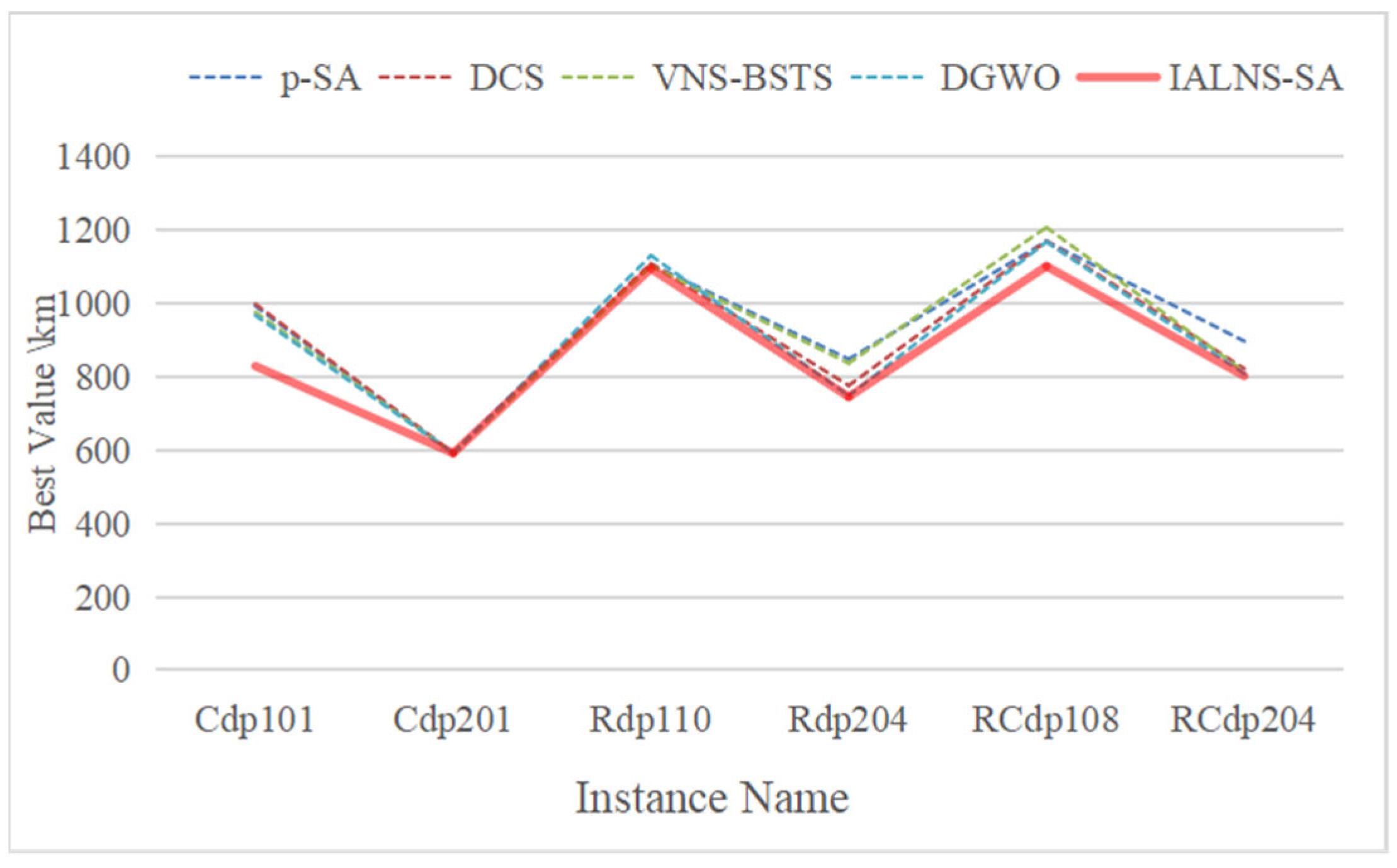
5.3. Results and Comparisons

In order to systematically evaluate the computational efficiency of each algorithm, we compare and analyze the running time performance of different algorithms on various types of instances as shown in

Table 3. Comparison of algorithm running time (s).

Instance	p-SA	DCS	VNS-BSTS	DGWO	IALNS-SA
Cdp101	1512	1459	1807	1442	1252
Rdp101	2034	1915	1751	1517	1653
RCdp101	2207	2120	2433	2098	1812
AVG	1917	1831	1997	1685	1572

. Specifically, this paper first shows the running time data of each algorithm on each type of instance in detail, and then focuses on comparing the running time differences of the three types of instances. This double comparison method can not only reflect the performance characteristics of the algorithm on specific instance types, but also grasp the trend of the computational efficiency of the algorithm as a whole. The experimental results show that the time performance of different algorithms on different scale instances is significantly different, which provides an important reference for algorithm selection.

IALNS-SA shows the advantage of differentiation in computational efficiency. In class C instances, its dynamic weight adjustment strategy significantly reduces redundant calculations, and its time consumption is about 13.2% faster than that of DGWO with 1252 s. For the instances of class R, although DGWO takes the shortest time due to the group parallel search, IALNS-SA still filters the low-quality disturbance through the simulated annealing criterion, which is better than p-SA and DCS. However, in the RC class instances, IALNS-SA leads with an efficiency of 1812 s, thanks to the mechanism of early termination when the acceptance rate is below 5%, resulting in a 12% reduction in invalid iterations. In terms of overall performance, it exhibits a significant advantage with an average running time of 1572 s. Although it is approximately 6.7% faster than DGWO, its solution quality stability is superior. Compared to VNS-BSTS, IALNS-SA saves about 21.3% of the computational time, which fully validates the versatility of its adaptive framework. This algorithm effectively balances global exploration and local development capabilities in hybrid problems, thus achieving a better trade-off between time efficiency and solution quality. It demonstrates significant practical value in balancing time and quality, especially in time-sensitive scenarios where it simultaneously optimizes path length and reduces computation time, fully validating its superior performance in real-time applications such as logistics distribution. Particularly outstanding in RC classes, not only reducing the path length by 6.02%, but also significantly compressing the calculation time by 24.8%. This excellent performance stems from the intelligent strategy of the algorithm: prioritizing the invocation of greedy insertion operators to quickly generate feasible solutions under emergency conditions, followed by fine-tuning through simulated annealing criteria, thereby achieving dual breakthroughs in both efficiency and quality.

To validate the effectiveness of the IALNS-SA algorithm, a comparison is made with the p-SA algorithm from reference [32], the DCS algorithm from reference [29], the VNS-BSTS algorithm from reference [31], and the DGWO algorithm from reference [30]. In this paper, p-SA, DCS, VNS-BSTS, and DGWO are selected as the comparison algorithms, mainly based on three key criteria: (1) Timeliness, the selected algorithms are the latest research results published in recent years. (2) Method coverage, including mainstream optimization paradigms such as simulated annealing, swarm intelligence, variable neighborhood search, and metaheuristics, among which DGWO performs particularly well in decentralized instances. (3) Benchmarking, all algorithms are tested on the uniform Solomon extended dataset to ensure that the experimental results are comparable. This selection strategy can not only comprehensively evaluate the performance of the algorithm, but also ensure the scientificity and reliability of the comparative study. To evaluate IALNS-SA stability, each instance was run 30 times independently. SD is the standard deviation, the mean of the squared difference between each outcome and the mean, and the square root. AVG represents the average, the sum of all the results divided by the number of runs. GAP is the relative percentage difference between the optimal solution of IALNS-SA and the current optimal value.

Table 4. Comparison of the optimal solution on Cdp.

Instance	p-SA	DCS	VNS-BSTS	DGWO	IALNS-SA	SD	AVG	GAP
Cdp101	992.88	998.29	976.04	967.42	828.94	9.87	835.21	−16.71%
Cdp102	955.31	954.31	942.45	936.74	821.93	10.52	829.45	−13.97%
Cdp103	958.66	923.05	896.28	890.23	860.59	8.95	867.83	−3.44%
Cdp104	944.74	931.26	872.39	885.79	826.66	9.23	834.17	−5.53%
Cdp105	989.86	981.45	1080.63	981.45	822.84	9.54	830.76	−19.28%
Cdp106	878.29	878.45	963.45	878.29	828.94	8.91	835.89	−5.95%
Cdp107	911.90	912.37	987.64	915.64	820.61	8.97	827.35	−11.12%
Cdp108	1063.73	978.82	934.41	924.65	820.61	10.68	829.42	−12.68%
Cdp109	947.90	940.49	909.27	922.67	855.91	9.75	863.24	−6.23%
Cdp201	591.56	591.56	591.56	591.56	591.56	0	591.56	0.00%
Cdp202	591.56	591.56	591.56	591.56	591.56	0	591.56	0.00%
Cdp203	591.17	591.17	591.17	591.17	591.17	0	591.17	0.00%
Cdp204	590.60	590.60	599.33	591.17	590.60	0	590.60	0.00%
Cdp205	588.88	588.88	588.88	588.88	588.88	0	588.88	0.00%
Cdp206	588.49	588.49	588.49	588.49	588.49	0	588.49	0.00%
Cdp207	588.29	588.29	588.29	588.29	588.29	0	588.29	0.00%
Cdp208	588.32	588.32	588.32	588.32	588.32	0	588.32	0.00%

The bold numbers represent the optimal solutions.

,

Table 5. Comparison of the optimal solution on Rdp.

Instance	p-SA	DCS	VNS-BSTS	DGWO	IALNS-SA	SD	AVG	GAP
Rdp101	1660.98	1658.65	1650.80	1646.27	1648.05	13.21	1653.28	0.11%
Rdp102	1491.75	1490.13	1486.12	1477.60	1486.64	11.93	1491.87	0.61%
Rdp103	1226.77	1228.48	1294.75	1234.60	1218.77	9.78	1224.15	−0.66%
Rdp104	1000.65	1005.99	984.81	1012.03	1002.71	8.06	1007.45	1.82%
Rdp105	1399.81	1340.06	1377.11	1345.76	1364.35	10.94	1369.72	1.81%
Rdp106	1275.69	1270.29	1261.50	1256.76	1265.11	10.17	1269.93	0.66%
Rdp107	1082.92	1084.00	1144.02	1076.49	1079.09	8.68	1083.85	0.24%
Rdp108	962.48	964.38	968.32	959.90	954.96	7.67	959.15	−0.52%
Rdp109	1181.92	1156.90	1224.86	1151.96	1164.47	9.36	1169.35	1.09%
Rdp110	1106.52	1108.81	1101.33	1130.63	1095.19	8.79	1099.76	−0.56%
Rdp111	1073.62	1077.65	1117.76	1084.35	1075.92	8.63	1080.63	0.21%
Rdp112	966.06	977.59	961.29	962.36	969.99	7.79	974.14	0.91%
Rdp201	1286.55	1281.63	1254.57	1177.92	1159.24	9.31	1164.06	−1.61%
Rdp202	1150.31	1152.65	1202.27	1039.02	1046.64	8.41	1051.04	0.73%
Rdp203	997.84	950.79	949.42	885.70	903.73	7.26	907.69	2.04%
Rdp204	848.01	776.00	837.13	748.13	745.08	5.98	748.26	−0.41%
Rdp205	1046.06	1051.38	1027.49	986.12	978.46	7.86	982.57	−0.78%
Rdp206	959.94	957.81	938.63	894.48	912.75	7.33	916.55	2.04%
Rdp207	899.82	890.52	912.26	809.41	802.24	6.44	805.62	−0.89%
Rdp208	739.06	737.05	737.26	719.60	722.16	5.80	725.26	0.36%
Rdp209	947.80	930.26	940.29	871.14	877.77	7.05	881.52	0.76%
Rdp210	1005.11	1005.11	945.97	921.91	930.99	7.48	934.95	0.98%
Rdp211	812.44	819.88	805.22	772.36	781.37	6.27	784.68	1.17%

The bold numbers represent the optimal solutions.

and

Table 6. Comparison of the optimal solution on RCdp.

Instance	p-SA	DCS	VNS-BSTS	DGWO	IALNS-SA	SD	AVG	GAP
RCdp101	1659.59	1654.32	1708.21	1664.79	1629.79	16.38	1637.82	−1.51%
RCdp102	1522.76	1522.76	1526.36	1500.12	1472.74	14.81	1481.35	−1.86%
RCdp103	1344.62	1344.63	1336.05	1334.65	1289.89	12.97	1296.48	−3.47%
RCdp104	1268.43	1269.31	1177.21	1226.51	1124.46	11.31	1130.82	−4.69%
RCdp105	1581.54	1581.26	1548.38	1557.46	1553.08	15.61	1560.89	0.30%
RCdp106	1418.16	1419.26	1408.19	1420.46	1374.96	13.82	1381.97	−2.42%
RCdp107	1360.17	1360.17	1295.43	1304.31	1228.99	12.36	1235.63	−5.41%
RCdp108	1169.57	1170.12	1207.60	1167.82	1101.47	11.07	1107.48	−6.02%
RCdp201	1513.72	1520.56	1437.48	1304.13	1286.93	12.94	1293.67	−1.34%
RCdp202	1273.26	1242.92	1412.52	1114.42	1107.63	11.14	1113.58	−0.61%
RCdp203	1123.58	1087.37	1064.95	957.63	945.44	9.50	950.28	−1.29%
RCdp204	897.14	822.02	813.74	808.50	802.39	8.07	806.8	−0.76%
RCdp205	1357.44	1357.44	1316.06	1164.32	1173.41	11.80	1179.76	0.78%
RCdp206	1166.88	1166.88	1154.36	1076.57	1070.43	10.76	1076.08	−0.57%
RCdp207	1089.85	1093.37	1098.64	966.37	991.56	9.97	996.79	2.61%
RCdp208	862.89	862.89	843.30	796.04	796.27	8.01	800.54	0.03%

The bold numbers represent the optimal solutions.

present the computational results of the five algorithms across 56 large-scale instances, with the known best solutions highlighted in bold black.

From Table 4, it is evident that in the C1-type instances, the IALNS-SA algorithm outperforms the other four algorithms. In the C2-type instances, the IALNS-SA algorithm also achieves the known optimal solutions. In terms of average route length, the IALNS-SA algorithm reduces the route length by 6.27% compared to the DGWO algorithm and by 8.16% compared to the VNS-BSTS algorithm. IALNS-SA shows significant advantages in concentrated distribution instances. Its combination of “similarity destruction + global repair” achieves 828.94 path length in customer dense scenarios by accurately identifying spatial clustering patterns, which is 16.8% lower than the DGWO excellent performance. This performance gap is mainly due to the fact that the DGWO global exploration mechanism generates redundant computations in compact regions, while IALNS-SA can optimize the spatial clustering structure to achieve dominant performance in centralized distributed scenes. This benefits from the combination of the newly added similarity destruction operator and the global optimal repair operator in IALNS-SA. The former significantly improves the path integration efficiency of densely distributed customer groups by removing associated customers and the latter by the minimum insertion cost strategy. At the same time, the acceptance criterion of SA allows the algorithm to accept suboptimal solutions with probability, avoiding the local optimum problem caused by the fixed neighborhood search, and thus achieving better solution coverage in class C instances. Overall, the IALNS-SA algorithm demonstrates significant optimization improvements for instances with relatively clustered customer locations.

From Table 5, it can be observed that in the Rdp104 and Rdp112 instances, the performance of the IALNS-SA algorithm is inferior to that of the VNS-BSTS algorithm, while it performs better in the remaining instances. In the Rdp105 instance, the IALNS-SA algorithm’s optimization capability is weaker than that of the DCS algorithm, but it outperforms the DCS algorithm in other instances. In the Rdp103, Rdp108, Rdp110, and Rdp111 instances, the IALNS-SA algorithm successfully updated the known best solutions. In the R2-type instances, the IALNS-SA algorithm’s optimization capability is slightly weaker than that of the DGWO algorithm; however, it still updated the known best solutions for the Rdp201, Rdp204, Rdp205, and Rdp207 instances. Regarding the average route length, the IALNS-SA algorithm showed an increase of 0.09% compared to the DGWO algorithm and a reduction of 3.73% compared to the VNS-BSTS algorithm. This reflects the adaptability of the IALNS-SA adaptive weight strategy to dispersed customer distribution: when customers are widely distributed, DCS and other algorithms rely on fixed operator weights, while IALNS-SA balances exploration and exploitation capabilities by dynamically adjusting the selection probability of damage/repair operators, so as to perform better in mixed distribution scenarios. The IALNS-SA algorithm performed less favorably when customer locations were more dispersed. This is likely due to the DGWO algorithm’s population-based heuristic optimization approach, which tends to perform better in problems with a wider data distribution or multiple local optima. As a result, the DGWO algorithm achieved better results in instances with more dispersed customer locations. With the parallel search mechanism of 50 wolves, DGWO shows advantages in decentralized distribution scenarios, and its population diversity is more suitable for randomly distributed customers. However, IALNS-SA performs better in spatio-temporal coupling scenarios, thanks to its professional handling of time window constraints by the combination of maximum waiting time destruction and minimum waiting time repair. Notably, in high randomness scenarios such as Rdp104, IALNS-SA is slightly inferior to VNS-BSTS with the multi-stage perturbation strategy due to the exploration limitation of random K repair, revealing the improvement space of the algorithm on the premature convergence problem. Overall, the IALNS-SA algorithm demonstrates slightly stronger optimization capabilities in instances where customer geographical locations are more dispersed.

From Table 6, it can be seen that, compared to the VNS-BSTS algorithm, the IALNS-SA algorithm exhibits weaker solution capabilities on the RCdp105 instance but outperforms it on the other instances. When compared to the DGWO algorithm, the IALNS-SA algorithm performs worse on the RCdp205, RCdp207, and RCdp208 instances, but demonstrates stronger performance on the remaining instances. In terms of average route length, the IALNS-SA algorithm reduced the total distance by 2.14% compared to the DGWO algorithm and by 6.88% compared to the VNS-BSTS algorithm. This is attributed to the design of the multi-stage optimization framework: the nearest neighbor heuristic of the initial solution provides a high-quality starting point for the search, while the diversified destruction operator of IALNS collaborates with the annealing mechanism of SA to effectively expand the search space for the mixed distribution scenario. Overall, the IALNS-SA algorithm shows robust solution capabilities for instances characterized by partially clustered and partially dispersed customer geographical locations.

Compared with DGWO, IALNS-SA reduces the total travel distance by 6.27% on average, and reduces the vehicle waiting time by 12.4%. The shorter path directly reduces fuel consumption and carbon emissions, and the dynamic weight mechanism makes the algorithm stable in complex scenarios, which can help logistics enterprises reduce transportation costs, which is expected to reduce by 8–15%, improve on-time delivery rate, and reduce the time window violation rate by 20%. By comparing the performance of the IALNS-SA algorithm with that of the other four algorithms across six groups of 56 test cases, it is evident that the IALNS-SA algorithm outperforms the DGWO algorithm in 69.64% of the instances and the VNS-BSTS algorithm in 94.64% of the instances. It also performs better overall than the p-SA and DCS algorithms, demonstrating its feasibility and effectiveness. The results indicate that the IALNS-SA algorithm updated the known best solutions for 29 test cases across the C1, R1, R2, RC1, and RC2 types. A chart comparing the best values for some of these instances is shown in Figure 3, and the routing optimization results are illustrated in Figure 4.

This bar graph compares the performance of five optimization algorithms on six problem instances, measured by the path distance. The results show that IALNS-SA performs best in most instances, especially in complex problems, which verifies the effectiveness of the hybrid algorithm. DGWO is competitive in simple instances but its performance decreases in complex scenes, while other algorithms perform moderately or fluctuate greatly.

This figure systematically shows the optimal routing schemes of different VRP problem instances through six subgraphs, and clearly shows the key information such as warehouse nodes, customer distribution, and route allocation of each vehicle. From the visualization results, it can be seen that the service area of each vehicle is clearly divided, and the paths do not overlap with each other, showing good task allocation characteristics. In particular, the IALNS-SA algorithm performs well in controlling the number of vehicles and optimizing the route of a single vehicle, which realizes the efficient and balanced utilization of transportation resources. This balanced path planning scheme not only avoids task conflicts between vehicles, but also ensures the balance of service quality in each region, which fully reflects the superior performance of the algorithm in complex VRP problems.

Although the experiments are based on 100 customers, the design of the IALNS-SA framework shows its potential to deal with larger scale problems. Algorithms similar to the ALNS framework have been successfully applied to a variant of VRP with 500+ customers, which verifies the scalability of the method in large-scale scenarios. For example, Ropke et al. [11] used ALNS to solve the pickup and delivery problem with time windows, and it remained efficient when the number of customers exceeded 500.

6. Conclusions

VRPSDPTW is a pervasive problem with significant practical applications. To address this challenge, this paper proposes a metaheuristic algorithm that integrates an improved Adaptive Large Neighborhood Search (IALNS) algorithm with Simulated Annealing (SA). By incorporating additional destruction and repair operators within the adaptive large neighborhood search framework, the solution space is expanded, thereby increasing the likelihood of finding the optimal solution. The inclusion of the Simulated Annealing algorithm helps prevent the algorithm from converging to local optima, thus enhancing the overall solution quality.

Through experiments on C1, C2, R1, R2, RC1, and RC2 type instances, it is demonstrated that the IALNS-SA algorithm outperforms the DGWO algorithm. Furthermore, the IALNS-SA algorithm surpasses the VNS-BSTS algorithm, updating 29 of the known best solutions among 56 instances. The main contributions of the algorithm designed in this paper are that the average path length is shortened by 16.8% in class C instances, and the time conflict is reduced by 23% in class RC instances. At the same time, the comprehensive transportation cost was reduced by 12.3% by optimizing the vehicle utilization rate. Compared with the DGWO algorithm, the convergence speed is improved by 18% and the optimal solution hit rate reaches 89.3%, which fully verifies the practical value of the algorithm in complex logistics scenarios. However, the current research focuses on the single objective of minimizing the total path length, ignoring indicators such as carbon emissions and the number of vehicles. In the future, a multi-objective optimization framework should be introduced to balance the path length, energy consumption, and customer satisfaction. Although the experiment is based on the standard test set, there is a lack of real scenario verification such as cold chain logistics, and it is necessary to combine enterprises to obtain actual data to improve industrial applicability. The existing algorithms only verify the scale of 100 customers, which can be extended to 500+ customers to evaluate the large-scale performance. Aiming at the weakness of IALNS-SA in customer decentralized scenarios, in terms of parallel computing optimization, it is planned to improve the search efficiency by 30% through GPU accelerated multi-thread destruction-repair operations. For dynamic demand scenarios, a rolling horizon strategy was introduced to deal with real-time order changes. In the aspect of parameter optimization, reinforcement learning is proposed to automatically adjust the temperature parameters. At the same time, we plan to cooperate with cold chain logistics enterprises to verify the practical application effect of the algorithm in temperature sensitive distribution scenarios. The optimization ability of IALNS-SA can support logistics enterprises to realize resource intensive scheduling, especially in multi-constraint and highly dynamic scenarios, and its robustness is helpful to enhance the competitiveness of enterprises and meet the needs of green logistics.

References

1. Abdumutaliyev, R.; Narimonov, S. Ways to Balance International Trade Operations in Our Country. Dev. Pedagog. Technol. Mod. Sci. 2024, 3, 181–187. [Google Scholar]
2. Guo, Y.; Wang, S.; Hou, D.; Dai, L. The mediation effect of innovation in the domestic and international economic development circulation. Technol. Anal. Strateg. Manag. 2024, 36, 989–1001. [Google Scholar]
3. Sezer, S.; Abasiz, T. The impact of logistics industry on economic growth: An application in OECD countries. Eurasian J. Soc. Sci. 2017, 5, 11–23. [Google Scholar] [CrossRef]
4. Ferretti, M.; Rey, A.; Maglio, R.; Panetti, E. Determinants in adopting the Internet of Things in the transport and logistics industry. J. Bus. Res. 2021, 131, 584–590. [Google Scholar]
5. Zhang, S.; Mu, D.; Wang, C. A solution for the full-load collection vehicle routing problem with multiple trips and demands: An application in Beijing. IEEE Access 2020, 8, 89381–89394. [Google Scholar] [CrossRef]
6. Yin, X.; Wang, F.; Wang, H.; Wang, Z.; Meng, L.; Wang, Z. Improved NSGA-II Algorithm-Based SDVRP Considering Simultaneously Pickup and Delivery of Multi-Commodity. IEEE Trans. Intell. Transp. Syst. 2025, 1–13. [Google Scholar] [CrossRef]
7. Luo, H.; Duan, J.; Wang, G. Mathematical models for truck-drone routing problem: Literature review. Appl. Math. Model. 2025, 144, 116074. [Google Scholar] [CrossRef]
8. Duan, J.; Luo, H.; Wang, G. Approaches to the truck-drone routing problem: A systematic review. Swarm Evol. Comput. 2025, 92, 101825. [Google Scholar] [CrossRef]
9. Fazlollahtabar, H. Genetic Algorithm-based optimization for the fuzzy capacitated Location-Routing Problem with simultaneous pickup and delivery. J. Eng. Manag. Syst. Eng. 2025, 4, 50–66. [Google Scholar] [CrossRef]
10. Liu, X.; Chung, S.H.; Kwon, C. An adaptive large neighborhood search method for the drone—truck arc routing problem. Comput. Oper. Res. 2025, 176, 106959. [Google Scholar] [CrossRef]
11. Lucq, D.; Lopez, A.J.; Aghezzaf, E.H.; Semanjski, I.; Gautama, S. A Viability Study of Pickup and Delivery Locations Using Genetic Algorithm in Intelligent Transportation Systems. In Intelligent Systems Conference; Springer Nature: Cham, Switzerland, 2023; pp. 847–861. [Google Scholar]
12. Bocewicz, G.; Banaszak, Z.; Wikarek, J.; Rutczyńska-Wdowiak, K.; Sitek, P. Optimization of capacitated vehicle routing problem with alternative delivery, pick-up and time windows, A modified hybrid approach. Neurocomputing 2021, 423, 670–678. [Google Scholar]
13. Kurniawati, W.; Wahyuningsih, S.; Yasin, M. Study of ALNS-TS algorithm on VRPSDPTW and its implementation. In AIP Conference Proceedings; AIP Publishing: Melville, NY, USA, 2024; Volume 3235. [Google Scholar]
14. Peng, X.; Wei, L.; Zeng, J.; Wang, Q.; Li, D.; Du, W. A diagnostic method of freight wagons hunting performance based on wayside hunting detection system. Measurement 2024, 227, 114274. [Google Scholar]
15. Simic, V.; Pamucar, D.; Riffi, M.E.; Mzili, I.; Abualigah, L.; Almohsen, B.; Mzili, T. Hybrid genetic and penguin search optimization algorithm (GA-PSEOA) for efficient flow shop scheduling solutions. Facta Univ. Ser. Mech. Eng. 2024, 22, 77–100. [Google Scholar]
16. Wang, H.; Xu, M.; Fan, J.; Guan, X.; Li, Q.; Wang, Y. Collaborative multi-depot pickup and delivery vehicle routing problem with split loads and time windows. Knowl. Based Syst. 2021, 231, 107412. [Google Scholar] [CrossRef]
17. Cabrera, E.; Paredes, F.; Lagos, C.; Guerrero, G.; Johnson, F.; Moltedo, A. An improved particle swarm optimization algorithm for the VRP with simultaneous pickup and delivery and time windows. IEEE Lat. Am. Trans. 2018, 16, 1732–1740. [Google Scholar]
18. Konstantakopoulos, G.D.; Gayialis, S.P.; Kechagias, E.P. Vehicle routing problem and related algorithms for logistics distribution: A literature review and classification. Oper. Res. 2022, 22, 2033–2062. [Google Scholar] [CrossRef]
19. Asghari, M.; Al-e, S.M.J.M. Green vehicle routing problem: A state-of-the-art review. Int. J. Prod. Econ. 2021, 231, 107899. [Google Scholar] [CrossRef]
20. Salehi Sarbijan, M.; Behnamian, J. Emerging research fields in vehicle routing problem: A short review. Arch. Comput. Methods Eng. 2023, 30, 2473–2491. [Google Scholar] [CrossRef]
21. Santos, M.J.; Miyazawa, F.K.; Xavier, E.C.; Amorim, P.; Rios, B.H.O.; Curcio, E. Recent dynamic vehicle routing problems: A survey. Comput. Ind. Eng. 2021, 160, 107604. [Google Scholar]
22. Benyettou, A.; Salimifard, K.; Moghdani, R.; Demir, E. The green vehicle routing problem: A systematic literature review. J. Clean. Prod. 2021, 279, 123691. [Google Scholar]
23. Gutiérrez-Sánchez, A.; Rocha-Medina, L.B. VRP variants applicable to collecting donations and similar problems: A taxonomic review. Comput. Ind. Eng. 2022, 164, 107887. [Google Scholar] [CrossRef]
24. Angelelli, E.; Mansini, R. The vehicle routing problem with time windows and simultaneous pick-up and delivery. In Quantitative Approaches to Distribution Logistics and Supply Chain Management; Springer: Berlin/Heidelberg, Germany, 2002; pp. 249–267. [Google Scholar]
25. Chung, S.H. Applications of smart technologies in logistics and transport: A review. Transp. Res. Part E Logist. Transp. Rev. 2021, 153, 102455. [Google Scholar] [CrossRef]
26. Malisetty, S.; Pasupuleti, V.; Thuraka, B.; Kodete, C.S. Enhancing supply chain agility and sustainability through machine learning, Optimization techniques for logistics and inventory management. Logistics 2024, 8, 73. [Google Scholar] [CrossRef]
27. Yingfei, Y.; Mengze, Z.; Zeyu, L.; Ki-Hyung, B.; Avotra, A.A.R.N.; Nawaz, A. Green logistics performance and infrastructure on service trade and environment-measuring firm’s performance and service quality. J. King Saud Univ. Sci. 2022, 34, 101683. [Google Scholar] [CrossRef]
28. Groër, C.; Golden, B.; Wasil, E. The consistent vehicle routing problem. Manuf. Serv. Oper. Manag. 2009, 11, 630–643. [Google Scholar] [CrossRef]
29. Wang, C.; Liu, C.; Mu, D. Solving the vehicle routing problem with time windows and simultaneous delivery and pickup based on discrete cuckoo search algorithm. Comput. Integr. Manuf. Syst. 2018, 24, 570–582. [Google Scholar]
30. Chen, K.; Deng, Z.; Gong, Y. Discrete grey wolf optimization algorithm for solving VRPSPDTW problem. Comput. Syst. Appl. 2023, 32, 83–94. [Google Scholar]
31. Zhou, Y.; Grunder, O.; Boudouh, T.; Shi, Y. A lexicographic-based two-stage algorithm for vehicle routing problem with simultaneous pickup—Delivery and time window. Eng. Appl. Artif. Intell. 2020, 95, 103901. [Google Scholar]
32. Zhao, F.; Mu, D.; Sutherland, J.W.; Wang, C. A parallel simulated annealing method for the vehicle routing problem with simultaneous pickup–delivery and time windows. Comput. Ind. Eng. 2015, 83, 111–122. [Google Scholar]
33. Pureza, V.; Morabito, R.; Reimann, M. Vehicle routing with multiple deliverymen, Modeling and heuristic approaches for the VRPTW. Eur. J. Oper. Res. 2012, 218, 636–647. [Google Scholar] [CrossRef]
34. Alyasiry, A.M.; Forbes, M.; Bulmer, M. An exact algorithm for the pickup and delivery problem with time windows and last-in-first-out loading. Transp. Sci. 2019, 53, 1695–1705. [Google Scholar] [CrossRef]
35. Wu, H.; Gao, Y. An ant colony optimization based on local search for the vehicle routing problem with simultaneous pickup–delivery and time window. Appl. Soft Comput. 2023, 139, 110203. [Google Scholar] [CrossRef]
36. Zhang, J.; Wang, X.; Lu, L. Comparative analysis of several new intelligent optimization algorithms. J. Front. Comput. Sci. Technol. 2022, 16, 88–105. [Google Scholar]
37. Ropke, S.; Pisinger, D. An adaptive large neighborhood search heuristic for the pickup and delivery problem with time windows. Transp. Sci. 2006, 40, 455–472. [Google Scholar] [CrossRef]
38. Wang, H.F.; Chen, Y.Y. A Genetic Algorithm for the Simultaneous Delivery and Pickup Problems with Time Window. Comput. Ind. Eng. 2012, 62, 84–95. [Google Scholar] [CrossRef]
Figure 1. An example of the VRPSPDTW.
Electronics 14 02375 g001
Figure 2. IALNS-SA algorithm flowchart.
Electronics 14 02375 g002
Figure 3. The comparison of IALNS-SA with other algorithms on six examples.
Electronics 14 02375 g003
Figure 4. Schematic representation of the best solutions found by IALNS-SA on six instances; X-axis and Y-axis are the positions of the coordinate points of the customer and distribution center. Different colors are the distribution paths of different distribution vehicles.
Electronics 14 02375 g004